2.1. Relevant results

Now, we recall the definitions of the Laplace transform and the translation transform:

Definition 1 The Laplace transform of a real-valued integrable function $\varphi (y), \ y\geq 0,$ is defined as

$$\tilde{\varphi}(s) = \int_0^{\infty} e^{{-}sy}\varphi(y)\,dy, \quad s>0.$$

Definition 2 The translation operator $T_s$ on a function $\varphi$ is defined by

(2.1)\begin{equation} T_s\varphi(x) = \int_x^{\infty} e^{{-}s(y-x)}\varphi(y)\,dy, \quad s>0. \end{equation}

Properties of the Laplace transform may be found in Chapter 1 of Spiegel [Reference Spiegel12].

2.2. The compound Poisson claim-counting process

Definition 3 We introduce the counting process $\{N(t), t\geq 0\}$ as follows:

$$N(t) = X_1 + \cdots + X_{M(t)}, \quad t\geq 0,$$

where $\{M(t), t\geq 0\}$ is a homogeneous Poisson process with intensity parameter $\lambda >0$ and probability mass function (p.m.f.) given by

$$\mathbb{P}\{M(t) = k\} = \frac{(\lambda t)^{k}}{k!}\,e^{-\lambda t}, \quad k=0,1,2,\ldots,$$

$\{X_1,X_2,\ldots \}$ are independent and identically distributed (i.i.d.) discrete random variables, which have the same p.m.f. $p_n,\ n=1,2,\ldots,$ as a generic random variable (r.v.) $X$, and are independent of $M(t)$.

It is noteworthy that Remark 2.1 in Li and Sendova [Reference Li and Sendova6] states that the process $N(t)$ is over-dispersed regardless of the distribution of $X$.

Definition 4 The surplus process $\{U(t), t \geq 0\}$ is given by

(2.2)\begin{equation} U(t) = u+ct-\sum^{N(t)}_{i=1}{Y_i}, \end{equation}

where $u \geq 0$ is the initial surplus and $c > 0$ is the constant premium rate. $\{Y_1,Y_2,\ldots \}$ are i.i.d. random variables, representing the successive individual claim amounts. $\{Y_1,Y_2,\ldots \}$ and $N(t)$ are further assumed to be mutually independent. We also denote by $F$ and $f$ the cumulative distribution function (c.d.f.) and the p.d.f., respectively, of the associated generic r.v. $Y$.

The surplus process $U(t)$ is based on the assumption that claims arrive according to a general compound Poisson process. The aggregate losses are then given by

$$S(t) = \sum_{i=1}^{N(t)} Y_i,\quad t\geq 0,$$

where $S(t)$ is a compound random variable with Laplace transform

$$\tilde{g}(s;t) = \mathcal{P}_{N(t)}[\tilde{f}(s)] =\mathcal{P}_{M(t)}\{\mathcal{P}_X[\tilde{f}(z)]\} = e^{-\lambda t \{1-\mathcal{P}_X[\tilde{f}(s)]\}},$$

where $\mathcal {P}_X$ denotes the p.g.f. of $X$.

In other words, $S(t)$ may be interpreted as a compound Poisson process with parameter $\lambda >0$ and compounded distribution having Laplace transform $\mathcal {P}_X[\tilde {f}(s)]$. Thus, the surplus process $U(t)$ defined in (2.2) may be regarded as a classical Poisson model with claim sizes having the latter Laplace transform. This is the same as having i.i.d. exponential inter-event times with mean $1/\lambda$, while each event is a compound r.v. that we will denote by $Z$. In other words, we have a number of i.i.d. claims occurring at the same time. Therefore, known results under the classical model also apply to the surplus process $U(t)$.

Let $F^{*n}(y)$ be the $n$-fold convolution of $F(y)$ with itself. Define $H(y)$ to be the c.d.f. of the compound r.v. $Z$, so that

$$H(y) = \sum^{\infty}_{n=1} p_n F^{*n}(y), \quad y\geq 0,$$

which is the c.d.f. of a batch claim. Subsequently, the p.d.f. and the survival function of $Z$ are denoted, respectively, by $h(y)$ and $\bar {H}(y)=1-H(y)$.

Also, $\mathbb {E}\{Z\} =\mu \mathbb {E}\{X\},$ where $\mu = \mathbb {E}\{Y\}$.

The Laplace transform of the associated p.d.f. is $\tilde {h}(s) = \mathcal {P}_X[\tilde {f} (s)],$ which is the p.g.f. of $X$ calculated at $\tilde {f} (s)$.

Define the equilibrium tail distribution of $Z$ as

$$H_e(y) = \frac{1}{\mathbb{E}\{Z\}} \int^{y} _0 \bar{H}(t)\,dt.$$

Then the associated p.d.f. is

$$h_e(y) = \frac{d}{dy}H_e(y) = \frac {\bar{H}(y)}{\mathbb{E}\{Z\}},$$

with Laplace transform

(2.3)\begin{equation} \tilde{h}_e(s) = \frac{1-\tilde{h}(s)}{s \mathbb{E}\{Z\}}. \end{equation}

We will further assume that the relative security loading $\theta$ satisfies the following relationship:

(2.4)\begin{align} ct & = (1+\theta) \mathbb{E}\left\{\sum_{i=1}^{N(t)}Y_i\right\} = (1+\theta) \mathbb{E}\{N(t)\}\mathbb{E}\{Y\}\nonumber\\ & = (1+\theta)\lambda t\mu\mathbb{E}\{X\}, \quad t \geq 0, \end{align}

where $c$ should satisfy the inequality

$$c > \lambda\mu\mathbb{E}\{X\},$$

to make sure $\theta$ is strictly positive.

2.3. Ruin-related quantities

2.3.1. The Gerber-Shiu function

Definition 5 The Gerber-Shiu function is defined by

$$m(u) = \mathbb{E}\{{e^{-\delta \tau} \omega(U(\tau-),|U(\tau)|)I(\tau< \infty) \,|\, U(0) = u}\}, \quad u \geq 0,$$

where $\delta \geq 0$ is a discount factor, $\tau = \inf \{t\geq 0 : U(t) <0\}$ is the time to ruin, $\omega (x, y)$, $x \geq 0$, $y>0$, is a penalty function, $U(\tau -)$ is the surplus before ruin, $|U(\tau )|$ is the deficit at ruin, and $I(\cdot )$ is the indicator function.

The Gerber-Shiu function was first introduced by Gerber and Shiu [Reference Gerber and Shiu5]. (See Eq. (2.10) there.)

Theorem 1 Let $\omega : [0,\infty )\times [0,\infty )\to [0,\infty )$ be a bounded (Borel-measurable) function, the relative security loading be positive, and the claim-size distribution have a finite second moment. Then, the Gerber-Shiu function satisfies the defective renewal equation

(2.5)\begin{equation} m(u) = \pi(\rho)\int_0^{u} m(u-y)\,dB(y;\rho)+\frac{\lambda}{c}T_\rho \zeta(u), \end{equation}

where $\rho$ is the non-negative root to the generalized Lundberg's fundamental equation

\begin{align*} & \lambda + \delta -cs = \lambda \tilde{h}(s),\\ & \pi(\rho) = \frac{\lambda}{c}\,T_\rho\bar{H}(0)\in (0,1),\\ & \zeta(u) = \int_u^{\infty} \omega(u,y-u)\,dH(y),\\ & \bar{B}(y;\rho) = 1-B(y;\rho) =\frac{T_\rho \bar{H}(y)}{T_\rho\bar{H}(0)}, \end{align*}

and $T_s f(y)$ is defined as in identity (2.1).

Equation (2.5) corresponds to identity (2.34) in Gerber and Shiu [Reference Gerber and Shiu5].

2.3.2. The ultimate ruin probability

We denote the ultimate ruin probability by

$$\psi (u) = \mathbb{P} \{\tau < \infty \,|\, U(0) = u \}.$$

Restating Eq. (4.11) in Gerber and Shiu [Reference Gerber and Shiu5], we have the following.

Corollary 2.1 When $\delta = 0$ and $\omega (x, y) = 1$ for all $x \geq 0,\ y >0$, the Gerber-Shiu function $m$ reduces to the probability of ultimate ruin $\psi$, which satisfies the defective renewal equation

(2.6)\begin{equation} \psi (u) = \frac {1}{1+ \theta} \int^{u}_0 \psi (u-t) \,dH_e(t) + \frac {1}{1+ \theta} \bar{H}_e(u), \quad u \geq 0. \end{equation}

The solution to (2.6) is the compound geometric survival function

$$\psi(u) = \frac{\theta}{1+\theta} \sum^{\infty}_{n = 1} \left(\frac{1}{1+ \theta}\right)^{n} \overline{H^{*n}}_e(u), \quad u \geq 0,$$

whose Laplace transform is

(2.7)\begin{equation} \tilde{\psi} (s) =\frac{1-\tilde{h}_e(s)}{s[1+\theta- \tilde{h}_e(s)]}. \end{equation}

We now make a connection with the $R_n$ family of distributions, i.e., those distributions whose Laplace transform of the respective p.d.f. is a rational function. As discussed in Subsection 2.1 of Sendova and Zhang [Reference Sendova and Zhang11], the $R_n$ class of distributions is fairly large and is not a subclass of the phase-type distributions.

Remark 1 According to the relationships among $\tilde {h}(s)$, $\tilde {h}_e(s)$ and $\tilde {\psi }(s)$ in equations (2.3) and (2.7), if the batch-claim distribution is in the $R_n$ family, then the resulting $\tilde {h}_e(s)$ and $\tilde {\psi }(s)$ are also in that family. Therefore, we are able to provide an explicit expression of the ultimate ruin probability. Consequently, more ruin-related quantities, such as the marginal moments of the time of ruin and the proper joint density of the surplus before ruin and the deficit at ruin are also expressed explicitly.

We formalize this observation in the following result:

Lemma 1 Whenever the distribution of batch claims belongs to the $R_n$ family of distributions, the probability of ruin also belongs to that family.

2.3.3. The defective joint density of the surplus before ruin and the deficit at ruin

The solution to the defective renewal Eq. (2.5) with $\delta = 0$ may be utilized to determine the defective joint density of the surplus before ruin and the deficit at ruin.

The defective joint density of the surplus before ruin and the deficit at ruin $f_d(x,y|u)$ was obtained in Section 7 in Dickson [Reference Dickson2].

We then deduce the proper joint density of the surplus before ruin and the deficit at ruin

(2.8)\begin{align} f(x,y\,|\,u) & = \frac{f_d(x,y\,|\,u)}{\int_0^{\infty} \int_0^{\infty} f_d(x,y\,|\,u) \,dy \,dx}\nonumber\\ & = \begin{cases} \displaystyle{\frac{[\psi(u)-\psi(u-x)]h(x+y)}{\mathbb{E}\{Z\}\int_{0}^{u}\bar{H}_e(u-t)\,d\psi(t)}}, & 0\le x< u,\ y>0 \\[6pt] \displaystyle{\frac{[\psi(u)-1]h(x+y)}{\mathbb{E}\{Z\}\int_{0}^{u}\bar{H}_e(u-t)\,d\psi(t)}}, & x>u,\ y>0 \end{cases},\quad u\ge 0. \end{align}

2.3.4. Marginal moments of the time of ruin

With the defective marginal moments $\psi _k$ for $k = 1,2,\ldots,$ given by

$$\psi_k(u) = \mathbb{E}\{\tau^{k}I(\tau<\infty)\,|\,U(0)=u\}, \quad u \geq 0,$$

we have the proper moments of the ruin time provided by

$$\frac{\psi_k(u)}{\psi(u)} = \mathbb{E}\{\tau^{k}\,|\,\tau<\infty, U(0)=u\}, \quad u \geq 0.$$

Then mean of the time of ruin is

$$\mathbb{E}\{\tau\,|\,\tau<\infty, U(0)=u\} = \frac{\psi_1(u)}{\psi(u)}, \quad u \geq 0,$$

its second moment is

$$\mathbb{E}\{\tau^{2}\,|\,\tau<\infty, U(0)=u\} = \frac{\psi_2(u)}{\psi(u)}, \quad u \geq 0,$$

and therefore, its variance is given as

$$\text{Var}\{\tau^{2}\,|\,\tau<\infty, U(0)=u\} = \frac{\psi_2(u)}{\psi(u)}-\left[\frac{\psi_1(u)}{\psi(u)}\right]^{2}, \quad u \geq 0.$$

As discussed in Section 6 of Willmot [Reference Willmot13], $\psi _1(u)$ satisfies the following difference equation

(2.9)\begin{equation} \psi_1(u) = \frac{1+\theta}{c\theta}\left[\int_0^{u} \psi(u-y)\psi(y)\,dy+\int_u^{\infty} \psi(y)\,dy-\psi(u)\int_0^{\infty}\psi(y)\,dy\right], \quad u \geq 0, \end{equation}

and $\psi _2(u)$ satisfies

(2.10)\begin{equation} \psi_2(u) = \frac{2(1+\theta)}{c\theta}\left[\int_0^{u} \psi_1(u-y)\psi(y)\,dy+\int_u^{\infty} \psi_1(y)\,dy-\psi(u)\int_0^{\infty}\psi_1(y)\,dy\right], \quad u \geq 0. \end{equation}

According to the Heaviside Expansion Theorem, which can be found on p. 46 of Spiegel [Reference Spiegel12], if the Laplace transform of $\psi (u)$ is of the form $\tilde {\psi }(s) = R(s)/P(s),$ where $R(s)$ is a polynomial of degree less than the degree of the polynomial $P(s),$ i.e., $\tilde {\psi }(s)$ is a rational function, and if $P(s)$ has $d$ distinct roots $\rho _j$, $j=1,2,\ldots,d,$ with negative real part, then the probability of ultimate ruin is given by

$$\psi(u) = \sum_{j=1}^{d} \frac{R(\rho_j)}{P'(\rho_j)}\,e^{\rho_j u}, \quad u \geq 0.$$

Therefore, $\psi _1(u)$ and $\psi _2(u)$ may be expressed explicitly as linear combinations of exponents.

3.1. Poisson-Geometric model (or Pólya-Aeppli model)

Now, assume that $X$ follows the zero-truncated geometric distribution with parameter $\beta$. We then have a Poisson-Geometric counting process $N(t)$.

The p.m.f. of $X$ is given by

$$p_n = \frac{\beta^{n-1}}{(1+\beta)^{n}},\quad \beta > 0,\ n=1,2,\ldots$$

Since $\text {Var}\{X\} / \mathbb {E}\{X\} = \beta$, then when $\beta <1,$ the zero-truncated geometric distribution is under-dispersed. Otherwise, it is over-dispersed. Therefore, this distribution can accommodate both over-dispersed and under-dispersed batch-claim arrivals.

3.1.1. General claim amounts

Now, we consider the most general case of the Poisson-Geometric model with the claim-size r.v. $Y$ following an unspecified distribution $f(y),\ y>0$. We derive some ruin-related quantities under this model.

Identity $\tilde {h}(s) = \mathcal {P}_X[\tilde {f} (s)]$ implies that the batch-claim amount distribution has Laplace transform

(3.1)\begin{align} \tilde{h}(s) & = \sum^ \infty _{n = 1} \frac{ \beta^{n-1}}{(1+ \beta)^{n}} [\tilde{f} (s)]^{n} \nonumber\\ & = \frac{\tilde{f}(s)}{1+\beta -\beta \tilde{f}(s)}. \end{align}

Equation (2.3), together with $\mathbb {E}\{Z\}=\mu (1+\beta )$, then produce

(3.2)\begin{equation} \tilde{h}_e(s) = \frac{1-\tilde{f}(s)}{\mu s [1+\beta-\beta\tilde{f}(s)]}.\end{equation}

Hence, with the help of (2.7), we have

(3.3)\begin{equation} \tilde{\psi} (s) = \frac{\mu s[1+\beta-\beta\tilde{f}(s)]-1+\tilde{f}(s)}{s\{\mu s(1+\theta)[1+\beta-\beta\tilde{f}(s)]-1+\tilde{f}(s)\}} . \end{equation}

Equation (2.4) results in the following expression for the relative security loading:

$$1+\theta=\frac{c}{\lambda\mu (1+\beta)}.$$

In the following two subsections, we consider the claim-size r.v. $Y$ following two specific distributions.

3.1.2. Exponential claim amounts

Assume $Y$ follows an exponential distribution with mean $\mu$, and p.d.f.

$$f(y)=\frac{1}{\mu}\,e^{-{y}/{\mu}}, \quad y \geq 0, \ \mu >0.$$

The Laplace transform of $f(y)$ is then

(3.4)\begin{equation} \tilde{f}(s) = \displaystyle{\frac{1}{1+ \mu s}}, \quad s\geq 0.\end{equation}

Hence, the Laplace transform of $h(y)$ is by (3.1)

$$\tilde{h}(s) = \frac{1}{1+ \mu s(1+ \beta)}.$$

Identity (3.2) then produces the Laplace transform of the equilibrium distribution

$$\tilde{h}_e(s) = \frac{1}{1+ \mu s(1+ \beta)}.$$

Notice that this indicates an exponential distribution with mean $1/\mu (1+\beta )$. Therefore, Eq. (3.3) produces

$$\tilde{\psi} (s) = \frac{({{1}/{\theta}})\mu(1+\beta)}{({{1}/{\theta}})\mu (1+\beta)(1+\theta)s+1}.$$

Inversion yields an explicit expression for the ultimate ruin probability. Namely,

$$\psi(u) = \frac{1}{1+\theta} \,e^{-{\theta u}/{\mu (1+\beta)(1+\theta)}}, \quad u \geq 0.$$

Hence, starting from (2.9), the defective mean of the time of ruin reduces to

$$\psi_1(u) =\frac{u+\mu(1+\beta)(1+\theta)}{c\theta(1+\theta)}\,e^{-{\theta u}/{\mu(1+\beta)(1+\theta)}},$$

which implies that the proper mean of the ruin time is

(3.5)\begin{equation} \mathbb{E}\{\tau\,|\,\tau<\infty, U(0)=u\} = \frac{u+\mu(1+\beta)(1+\theta)}{c\theta}. \end{equation}

Similarly, implementing identity (2.10), the defective second moment of the time of ruin is given by

$$\psi_2(u) =\frac{\theta u^{2} +2\mu(1+\beta)(1+\theta)(1+2\theta)u+2\mu^{2}(1+\beta)^{2}(1+\theta)^{3}}{c^{2}\theta^{3}(1+\theta)}\,e^{-{\theta u}/{\mu(1+\beta)(1+\theta)}},$$

and the second moment of the ruin time is

(3.6)\begin{equation} \mathbb{E}\{\tau^{2}\,|\,\tau<\infty, U(0)=u\} = \frac{\theta u^{2} +2\mu(1+\beta)(1+\theta)(1+2\theta)u+2\mu^{2}(1+\beta)^{2}(1+\theta)^{3}}{c^{2}\theta^{3}}. \end{equation}

Therefore, from (3.5) and (3.6), the variance of the time of ruin is

$$\text{Var}\{\tau^{2}\,|\,\tau<\infty, U(0)=u\} = \frac{2\mu(1+\beta)(1+\theta)^{2}u+\mu^{2}(1+\beta)^{2}(1+\theta)^{2}(2+\theta)}{c^{2}\theta^{3}}.$$

Observe that the mean and the variance of the ruin time are linear functions of $u$.

Finally, (2.8) provides the proper joint density of the surplus before ruin and the deficit at ruin

$$f(x,y\,|\,u)=\begin{cases} \displaystyle{\frac{(1+\theta)\lambda}{c\theta \mu (1+\beta)}}[e^{{\theta x}/{\mu(1+\beta)(1+\theta)}}-1]\,e^{-{(x+y)}/{\mu(1+\beta)}}, & 0 \leq x< u,\ y>0\\[6pt] \displaystyle{\frac{(1+\theta)\lambda}{c\theta\mu (1+\beta)}}[(1+\theta)\,e^{{\theta u}/{\mu(1+\beta)(1+\theta)}}-1]\,e^{-{(x+y)}/{\mu(1+\beta)}}, & x> u,\ y>0 \end{cases},\quad u\ge 0.$$

Interestingly, the above density depends on the initial surplus only through its relative position with respect to the surplus before ruin.

3.1.3. Erlang($k$) claim amounts

Assume $Y$ follows an Erlang($k$) distribution with mean of $k\mu$, and p.d.f.

$$f(y)=\frac{1}{\mu^{k} k!} y^{k-1}\,e^{-{y}/{\mu}}, \quad y \geq 0 ,\ \mu >0.$$

Then, we obtain the Laplace transform of $f(y)$

(3.7)\begin{equation} \tilde{f}(s) = \frac{1}{(1+ \mu s)^{k}}, \quad s\geq 0. \end{equation}

The Laplace transform $\tilde {h}(s)$ is expressed from (3.1) as

$$\tilde{h}(s) = \frac{1}{(1+\beta)(1+ \mu s)^{k}- \beta}.$$

Applying the Heaviside Expansion Theorem, if there are $n$ roots $\eta _1,\ldots,\eta _n$ with negative real parts, which are all distinct, $h(y)$ is then

$$h(y) = \sum_{j=1}^{n} \frac{1}{k \mu (1+\beta)(1+\mu \eta_j)^{k-1}}\,e^{\eta_j y}.$$

Applying $\mathbb {E}\{Z\}=k\mu (1+\beta )$ and Eq. (3.2), $\tilde {h}_e(s)$ is then

$$\tilde{h}_e(s) =\frac{(1+\mu s)^{k}-1}{k\mu s[(1+\beta)(1+\mu s)^{k}-\beta]}.$$

Hence, with the help of (3.3) with $\mu$ replaced by $k\mu,$ we have

$$\tilde{\psi} (s) = \frac{k\mu s[(1+\beta)(1+\mu s)^{k} - \beta]-(1+\mu s)^{k}+1}{s\{k\mu s(1+\theta)[(1+\beta)(1+\mu s)^{k}-\beta]-(1+\mu s)^{k}+1\}},$$

and the relative security loading is

$$1+\theta=\frac{c}{k\lambda\mu (1+\beta)}.$$

Observe that $\tilde {\psi }(s)$ may be presented as $\tilde {\psi }(s) = R(s)/P(s),$ and then the Heaviside Expansion Theorem applies. If the polynomial $P(s)$ has $m$ distinct roots $\rho _1, \rho _2,\ldots,\rho _m$ with negative real parts, then the probability of ultimate ruin is given explicitly by

$$\psi(u) = \sum_{j=1}^{m} \frac{R(\rho_j)}{P'(\rho_j)}\,e^{\rho_j u},$$

where

$$R(\rho_j) = k\mu \rho_j[(1+\mu \rho_j)^{k} - \beta]-(1+\mu \rho_j)^{k}+1,$$

and

\begin{align*} P'(\rho_j) & = k\mu\rho_j(1+\theta)(1+\beta)(1+\mu\rho_j)^{k-1}(2+2\mu\rho_j+k \mu\rho_j)\\ & \quad -2k \beta (1+\theta)\mu\rho_j-(1+\mu\rho_j)^{k-1}(1+\mu \rho_j+k\mu \rho_j)+1. \end{align*}

Finally, the proper joint density of the surplus before ruin and the deficit at ruin is

\begin{align*} & f(x,y|u) =\begin{cases} \displaystyle{\frac{\sum_{i=1}^{n}\sum_{j=1}^{m} \frac{1}{k^{2} \mu^{2} (1+\beta)^{2}(1+\mu \eta_i)^{k-1}}\frac{R(\rho_j)}{P'(\rho_j)}\,e^{\eta_i (x+y)+\rho_j u}(1-e^{-\rho_j x})}{\sum_{j=1}^{m} \frac{R(\rho_j)}{P'(\rho_j)}(e^{\rho_j u}-1)-\sum_{i=1}^{n}\sum_{j=1}^{m} \frac{(1+\mu \eta_i)^{k}-1}{k\mu\eta_i\left[(1+\beta)(1+\mu \eta_i+k \mu \eta_i)(1+\mu \eta_i)^{k-1}-\beta\right]}\frac{R(\rho_j)}{P'(\rho_j)}\left[\frac{\eta_i}{\rho_j-\eta_i}e^{\rho_j u}-\frac{\rho_j}{\rho_j-\eta_i}e^{\eta_i u}+1\right]}}, \\ {\rm where} \ 0\le x< u,\ y>0,\\ \displaystyle{\frac{\sum_{i=1}^{n} \frac{1}{k^{2} \mu^{2} (1+\beta)^{2}(1+\mu \eta_i)^{k-1}}\,e^{\eta_i (x+y)}\left[\sum_{j=1}^{m} \frac{R(\rho_j)}{P'(\rho_j)}e^{\rho_j u}-1\right]}{\sum_{j=1}^{m} \frac{R(\rho_j)}{P'(\rho_j)}(e^{\rho_j u}-1)-\sum_{i=1}^{n}\sum_{j=1}^{m} \frac{(1+\mu \eta_i)^{k}-1}{k\mu\eta_i\left[(1+\beta)(1+\mu \eta_i+k \mu \eta_i)(1+\mu \eta_i)^{k-1}-\beta\right]}\frac{R(\rho_j)}{P'(\rho_j)}\left[\frac{\eta_i}{\rho_j-\eta_i}e^{\rho_j u}-\frac{\rho_j}{\rho_j-\eta_i}e^{\eta_i u}+1\right]}}, \\ {\rm where} \ x>u,\ y>0 \end{cases}. \end{align*}

with the help of (2.8).

3.2. Poisson-Negative-Binomial model

Assume that $X$ follows the zero-truncated negative-binomial distribution with parameters $\alpha$ and $r$. Then we call this risk model a Poisson-Negative-Binomial risk model as the counting process $N(t)$ is a Poisson-Negative-Binomial process.

The p.m.f. of $X$ is

$$p_n = \frac{1}{(1+\alpha)^{r}-1}\dbinom{r+n-1}{n}\left(\frac{\alpha}{1+\alpha}\right)^{n},\quad r>{-}1,\ r \ne 0,\ \alpha > 0,\ n=1,2,\ldots$$

When $\alpha <(1+r)^{{1}/{r}-1}$, the zero-truncated negative-binomial distribution is under-dispersed. Otherwise, it is over-dispersed. Therefore, this distribution can accommodate both over-dispersed and under-dispersed batch arrivals.

3.2.1. General claim amounts

Now, we consider the most general case of the Poisson-Negative-Binomial model with the claim-size r.v. $Y$ following a general distribution. We then derive some ruin-related quantities under this model.

The Laplace transform of $h(y)$ is deducted to be

\begin{align*} \tilde{h}(s) & = \frac{1}{(1+\alpha)^{r}-1}\sum^ \infty _{n = 1} \dbinom{r+n-1}{n}\left(\frac{\alpha}{1+\alpha}\right)^{n} [\tilde{f} (s)]^{n} \\ & = \frac{1}{(1+\alpha)^{r}-1} \left\{\frac{1}{[1-({{\alpha}/{(1+\alpha)}})\tilde{f} (s)]^{r}}-1 \right\}. \end{align*}

With $\mathbb {E}\{Z\}={\mu r \alpha }/{(1-(1+\alpha )^{-r})}$ and (2.3), $\tilde {h}_e(s)$ is expressed as

(3.8)\begin{equation} \tilde{h}_e(s) = \frac{1}{\mu r\alpha s}\left\{1-\frac{1}{[1+\alpha-\alpha\tilde{f}(s)]^{r}}\right\}.\end{equation}

Therefore, Eq. (2.7) reduces to

(3.9)\begin{equation} \tilde{\psi} (s) = \frac{(\mu r \alpha s-1)[1+\alpha-\alpha\tilde{f}(s)]^{r}+1}{s\{[(1+\theta)\mu r \alpha s-1][1+\alpha-\alpha\tilde{f}(s)]^{r}+1\}},\end{equation}

with relative security loading

$$1+\theta=\frac{c[1-(1+\alpha)^{{-}r}]}{\lambda\mu r \alpha}.$$

3.2.2. Exponential claim amounts

Assume $Y$ follows an exponential distribution with mean $\mu$. From the results obtained in Section 5.1.1 in Li and Sendova [Reference Li and Sendova6], the Laplace transform of $h(y)$ is given by

$$\tilde{h}(s) = \frac{1}{(1+\alpha)^{r}-1}\left\{\left[\frac{(1+\alpha)(1+\mu s)}{1+(1+\alpha)\mu s}\right]^{r}-1\right\}.$$

By identity (3.8), the Laplace transform of $h_e(y)$ is

$$\tilde{h}_e(s) =\frac{1}{\mu r \alpha s}\left\{1-\left[\frac{1+\mu s}{1+(1+\alpha)\mu s}\right]^{r}\right\}.$$

The Laplace transform of the probability of ultimate ruin is obtained by Eq. (3.9) and formula (3.4) to be

$$\tilde{\psi} (s) = \frac{(s\mu r \alpha -1)[1+(1+\alpha)\mu s]^{r}+(1+\mu s)^{r}}{s\{[s\mu r \alpha (1+\theta)-1][1+(1+\alpha)\mu s]^{r}+(1+\mu s)^{r}\}},$$

which recovers Eq. (35) in Li and Sendova [Reference Li and Sendova6]. Moreover, as $\tilde {\psi }(s)$ is a rational function, $\psi (u)$ may be presented as a linear combination of exponentials as is done in Eq. (38) in Li and Sendova [Reference Li and Sendova6].

Finally, the proper joint density of the surplus before ruin and the deficit at ruin is calculated through (2.8), where

\begin{align*} & \int_0^{u}\bar{H}_e(u-t)\,d\psi(t) \\ & \quad =\sum_{j=1}^{m}\frac{R(\rho_j)}{P'(\rho_j)}\left\{\left[1-\frac{1-(1+\alpha)^{{-}r}}{\mu r \alpha \rho_j}\right](e^{\rho_j u}-1)+\frac{1-(1+\alpha)^{{-}r}}{\mu r \alpha }u\right\}\\ & \qquad +\frac{1}{\mu r \alpha (1+\alpha)^{r}}\sum_{i=1}^{r} \sum_{j=1}^{m}\dbinom{r}{i} \alpha^{i} \frac{R(\rho_j)}{P'(\rho_j)}\left[\left(\frac{1}{\rho_j}-i\right)(e^{\rho_j u}-1)-u\right]\\ & \qquad-\frac{1}{\mu r \alpha (1+\alpha)^{r}}\sum_{i=1}^{r} \sum_{w=0}^{i-1} \sum_{n=0}^{w} \sum_{j=1}^{m} \sum_{h=0}^{n}\dbinom{r}{i}\alpha^{i} \frac{R(\rho_j)}{P'(\rho_j)}\frac{\rho_j}{(n-h)!} \frac{[(1+\alpha)\mu]^{h-n+1}u^{n-h}}{[(1+\alpha)\mu\rho_j+1]^{h+1}}\,e^{- {u}/{\mu(1+\alpha)}}. \end{align*}

3.2.3. Erlang($k$) claim amounts

Assume $Y$ follows an Erlang($k$) distribution with mean $k\mu$. Therefore, identity (3.9) together with formula (3.7) imply that

$$\tilde{\psi} (s) = \frac{(k\mu r \alpha s -1)[(1+\alpha)(1+\mu s)^{k}-\alpha]^{r}+(1+\mu s)^{kr}}{s\{[(1+\theta)k\mu r \alpha s-1][(1+\alpha)(1+\mu s)^{k}-\alpha]^{r}+(1+\mu s)^{kr}\}},$$

which is the result of Subsection 5.1.2 in Li and Sendova [Reference Li and Sendova6]. We may then write $\tilde {\psi }(s) = R(s)/P(s)$, where $R$ and $P$ are known polynomials. If $P(s)$ has $m$ distinct roots $\rho _1, \rho _2,\ldots,\rho _m$ with negative real parts, then the Heaviside Expansion Theorem implies that the probability of ultimate ruin is given explicitly by

$$\psi(u) = \sum_{j=1}^{m} \frac{R(\rho_j)}{P'(\rho_j)}\,e^{\rho_j u},$$

where

$$R(\rho_j) = (k\mu r \alpha \rho_j -1)[(1+\alpha)(1+\mu \rho_j)^{k}-\alpha]^{r}+(1+\mu \rho_j)^{kr},$$

and

\begin{align*} P'(\rho_j) & = \mu kr\rho_j (1+\alpha)(1+\mu \rho_j)^{k-1}[k\mu\rho_j r \alpha(1+\theta)-1][(1+\alpha)(1+\mu \rho_j)^{k}-\alpha]^{r-1} \\ & \quad +[2k\mu\rho_j r \alpha(1+\theta)-1][(1+\alpha)(1+\mu \rho_j)^{k}-\alpha]^{r}+ [\rho_j \mu(kr+1)+1](1+\mu\rho_j)^{kr-1}. \end{align*}

Note that here the relative security loading is

$$1+\theta=\frac{c[1-(1+\alpha)^{{-}r}]}{k\lambda\mu r \alpha}.$$

3.3. Poisson-Binomial model

Assume that $X$ follows the zero-truncated binomial distribution with parameters $l$ and $q$. Then the risk model is called a Poisson-Binomial risk model with a Poisson-Binomial counting process $N(t)$.

The p.m.f. of $X$ is given by

$$p_n = \frac{\dbinom{l}{n}q^{n}(1-q)^{l-n}}{1-(1-q)^{l}},\quad 0< q<1,\ l = 1,2,\ldots,\ n=1,2,\ldots,l.$$

The zero-truncated binomial distribution is under-dispersed, which means that this distribution may only accommodate under-dispersed batch arrivals.

3.3.1. General claim amounts

We now consider the most general case of the Poisson-Binomial model with the claim-size r.v. $Y$ following a general distribution. Then, we derive some ruin-related quantities under this model.

The Laplace transform of $h(y)$ is expressed as

$$\tilde{h}(s) = \sum^ \infty _{n = 1} \frac{\dbinom{l}{n}q^{n}(1-q)^{l-n}}{1-(1-q)^{l}}[\tilde{f} (s)]^{n} =\frac{(1-q)^{l}}{1-(1-q)^{l}}\left\{\frac{1}{[1-({q}/{(1-q)})\tilde{f} (s)]^{l-n+1}}-1 \right\}.$$

Since $\mathbb {E}\{Z\}={\mu l q}/{(1-(1-q)^{l})}$ and from (2.3), we have

(3.10)\begin{equation} \tilde{h}_e(s) = \frac{1}{\mu l q s}\left\{1-\frac{(1-q)^{2l-n+1}}{[1-q-q\tilde{f} (s)]^{l-n+1}}\right\}.\end{equation}

Hence, identity (2.7) yields the Laplace transform of the ruin time

(3.11)\begin{equation} \tilde{\psi} (s) = \frac{(\mu lq s-1)[1-q-q\tilde{f} (s)]^{l-n+1}+(1-q)^{2l-n+1}}{s\{[(1+\theta)\mu lq s-1][1-q-q\tilde{f} (s)]^{l-n+1}+(1-q)^{2l-n+1}\}},\end{equation}

with relative security loading

$$1+\theta=\frac{c[1-(1-q)^{l}]}{\lambda\mu lq}.$$

3.3.2. Exponential claim amounts

Assume $Y$ follows the exponential distribution with mean $\mu$. From the results obtained in Section 5.2.1 in Li and Sendova [Reference Li and Sendova6], the Laplace transform of $h(y)$ is given by

$$\tilde{h}(s) = \frac{(1-q)^{l}}{1-(1-q)^{l}}\left\{\left[\frac{1+(1-q)\mu s}{(1-q)(1+\mu s)}\right]^{l}-1\right\}.$$

Thus, we obtain the Laplace transform of $h_e(y)$

$$\tilde{h}_e(s) = \frac{1}{\mu lq s}\left\{1-\left[\frac{1+(1-q)\mu s}{1+\mu s}\right]^{l}\right\}$$

by Eq. (3.10). With the help of Eqs. (3.11) and (3.4), the Laplace transform of the probability of ultimate ruin is

$$\tilde{\psi} (s) = \frac{(\mu lqs -1)(1+\mu s)^{l}+[1+\mu s(1-q)]^{l}}{s\{[\mu lqs (1+\theta)-1](1+\mu s)^{l}+[1+\mu s(1-q)]^{l}\}},$$

which recovers identity (44) in Li and Sendova [Reference Li and Sendova6]. Subsequently, as $\tilde {\psi }(s)$ is a rational function, $\psi (u)$ may be presented as a linear combination of exponentials as is done in Li and Sendova [Reference Li and Sendova6].

Finally, the proper joint density of the surplus before ruin and the deficit at ruin is given in (2.8), where

\begin{align*} \int_0^{u}\bar{H}_e(u-t)d\psi(t) & = \sum_{j=1}^{m}\frac{R(\rho_j)}{P'(\rho_j)}\left[\left(1-\frac{1-(1-q)^{l}}{\mu l q \rho_j}\right)(e^{\rho_j u}-1)+\frac{1-(1-q)^{l}}{\mu l q }u\right]\\ & \quad +\frac{1}{\mu l q}\sum_{i=1}^{l} \sum_{j=1}^{m}\dbinom{l}{i}q^{i}(1-q)^{l-i} \frac{R(\rho_j)}{P'(\rho_j)}\left[\left(\frac{1}{\rho_j}-i\right)(e^{\rho_j u}-1)-u\right]\\ & \quad +\frac{1}{\mu l q}\sum_{i=1}^{l} \sum_{w=0}^{i-1} \sum_{n=0}^{w} \sum_{j=1}^{m} \sum_{h=0}^{n}\dbinom{l}{i}q^{i}(1-q)^{l-i} \frac{R(\rho_j)}{P'(\rho_j)}\frac{\rho_j}{(n-h)!} \frac{\mu^{h-n+1}u^{n-h}}{(\mu\rho_j+1)^{h+1}}e^{-{u}/{\mu}}. \end{align*}

3.3.3. Erlang($k$) claim amounts

Assume $Y$ follows an Erlang($k$) distribution with mean $k\mu$. From the results obtained in Section 5.1.2 in Li and Sendova [Reference Li and Sendova6], the Laplace transform of $h(y)$ is

$$\tilde{h}(s) = \frac{(1-q)^{l}}{1-(1-q)^{l}}\left\{\left[\frac{(1-q)(1+\mu s)^{k}+q}{(1-q)(1+\mu s)^{k}}\right]^{l}-1\right\},$$

since $\mathbb {E}\{Z\}={k\mu l q}/{(1-(1-q)^{l})}$ and (3.10), the Laplace transform of $h_e(y)$ is

$$\tilde{h}_e(s) = \frac{1}{k\mu lq s}\left\{1-\left[\frac{(1-q)(1+\mu s)^{k}+q}{(1+\mu s)^{k}}\right]^{l}\right\}.$$

Hence, we obtain the Laplace transform of the probability of ultimate ruin through Eqs. (3.11) and (3.7):

$$\tilde{\psi} (s) = \frac{(k\mu lqs -1)(1+\mu s)^{kl}+[(1-q)(1+\mu s)^{k}+q]^{l}}{s\{[k\mu lq s(1+\theta)-1](1+\mu s)^{kl}+[(1-q)(1+\mu s)^{k}+q]^{l}\}},$$

which recovers the relevant expression in Subsection 5.2.2 in Li and Sendova [Reference Li and Sendova6] and $\psi (u)$ may be again presented as a known linear combination of exponentials. Namely,

$$\psi(u) = \sum_{j=1}^{m} \frac{R(\rho_j)}{P'(\rho_j)}\,e^{\rho_j u},$$

where

$$R(\rho_j) = (k\mu lq\rho_j -1)(1+\mu \rho_j)^{kl}+[(1-q)(1+\mu \rho_j)^{k}+q]^{l},$$

and

\begin{align*} P'(\rho_j) & =\{\mu kl\rho_j [k\mu\rho_j lq(1+\theta)-1]+ [2k\mu\rho_j lq(1+\theta)-1](1+\mu \rho_j)\}(1+\mu \rho_j)^{kl-1} \\ & \quad + \{[1+\mu \rho_j(1+kl)](1-q)(1+\mu \rho_j)^{k-1}+q\}[(1-q)(1+\mu\rho_j)^{k}+q]^{l-1}. \end{align*}

Here, the relative security loading is

$$1+\theta=\frac{c[1-(1+\alpha)^{{-}r}]}{k\lambda\mu r \alpha}.$$

Finally, the proper joint density of the surplus before ruin and the deficit at ruin is given in (2.8), where

\begin{align*} \int_0^{u}\bar{H}_e(u-t)\,d\psi(t) & = \sum_{j=1}^{m}\frac{R(\rho_j)}{P'(\rho_j)}\left[\left(1-\frac{1-(1-q)^{l}}{k\mu l q \rho_j}\right)(e^{\rho_j u}-1)+\frac{1-(1-q)^{l}}{k\mu l q }u\right]\\ & \quad +\frac{1}{k\mu l q}\sum_{i=1}^{l} \sum_{j=1}^{m}\dbinom{l}{i}q^{i}(1-q)^{l-i} \frac{R(\rho_j)}{P'(\rho_j)}\left[\left(\frac{1}{\rho_j}-i\right)(e^{\rho_j u}-1)-u\right]\\ & \quad +\frac{1}{k\mu l q}\sum_{i=1}^{l} \sum_{w=0}^{ki-1} \sum_{n=0}^{w} \sum_{j=1}^{m} \sum_{h=0}^{n}\dbinom{l}{i}q^{i}(1-q)^{l-i} \frac{R(\rho_j)}{P'(\rho_j)}\frac{\rho_j}{(n-h)!} \frac{\mu^{h-n+1}u^{n-h}}{(\mu\rho_j+1)^{h+1}}\,e^{- {u}/{\mu}}. \end{align*}

4.1. Exponential claim amounts

In this subsection, we focus on examples with exponentially distributed claim amounts.

We firstly consider an example in the case of zero-truncated geometric batch arrivals.

As stated in Section 3, zero-truncated geometric batch arrivals may accommodate both under- and over-dispersed data, while the resulting Poisson-Geometric counting process is always over-dispersed. In other words, no matter whether the insurance company receives an under- or over-dispersed number of claims at a time, the total number of claims is always over-dispersed. When $\beta = 0.5$, the batch arrivals are under-dispersed, while when $\beta = 2$ or 10, the batch arrivals are over-dispersed. In order to measure the efficiency of the compound Poisson model, we also consider the case $\beta = 0,$ which results in no-batch arrivals and serves for comparison. The c.d.f. of the zero-truncated geometric distribution in the four cases for $\beta$ is plotted in Figure 1. As the plot shows, the model whose batch arrivals follow the zero-truncated geometric distribution with larger $\beta$ is more likely to receive larger number of claims at a time. This means that an insurance company with more business requires a model with a larger $\beta$. Note that the scale of the liabilities of the insurance company does not only depend on the number of claims per day but also depend on the amount of each claim.

Figure 1.

C.d.f. of the zero-truncated geometric distribution.

The probability of ultimate ruin for different $\beta$ is then plotted in Figure 2. Ideally, the ultimate ruin probability should be below $5\%$. This is why we add a horizontal line at $5\%$ on the plot. Intuitively, the probability of ultimate ruin should decrease with the increase of the initial surplus. In the extreme case, if the insurance company starts with an infinite initial surplus, then there is no risk of ruin. This is confirmed in Figure 2. Moreover, the approximate values of $u$ for $\psi (u) = 0$ and $5\%$ for four different values of $\beta$ are summarized in Table 1. According to the table, we have seen that for the same level of initial surplus, the larger the $\beta$, the larger the probability of ruin is. Thus, over-dispersed batch arrivals correspond to a higher risk of ruin. In general, Figure 2 demonstrates that the possibility of batch-claim arrivals should not be underestimated as it influences the probability of ruin in a substantial way. We also observed that the approximate value of $u$ when the probability of ultimate ruin falls to $5\%$ is approximately half of that when the probability of ultimate ruin reaches zero, especially when $\beta$ is small. This indicates that in order to maintain a relatively low risk of ruin, the insurance companies may only need half of the initial surplus required for reducing the risk of ruin to an exceedingly smaller level.

Figure 2.

Probability of ultimate ruin.

Table 1.

Approximate values of $u$ for which the respective values for $\psi$ are reached for the first time.

The mean and variance of the ruin time are plotted in Figures 3 and 4, respectively. These plots illustrate what we already know from Eqs. (3.5) and (3.6), which is that both the mean and the variance of the ruin time are linear functions of the initial surplus. We also observe that for the same level of the initial surplus, the model with a higher $\beta$ corresponds to lower mean and variance of the ruin time. In other words, over-dispersed batch arrivals lead to shorter ruin time. This is another evidence that the possibility of batch arrivals should not be underrated when building a model.

Figure 3.

Mean of the ruin time.

Figure 4.

Variance of the ruin time.

Assume that $u=25$. The proper joint density of the surplus before ruin and the deficit at ruin for different $\beta$ are plotted in Figure 5. It seems that most frequently, ruin occurs when the current surplus drops below the initial surplus. When $\beta$ is larger, ruin may also happen when the current surplus is larger than the initial surplus. Besides, the joint density comes to a higher peak when $\beta$ is small. It shows that when the Poisson-Geometric model is employed, especially for over-dispersed batch arrivals, ruin happens more dispersedly compared with the no-batch-arrivals case ($\beta =0$).

Figure 5.

Proper joint density of the surplus before ruin and the deficit at ruin for different $\beta$.

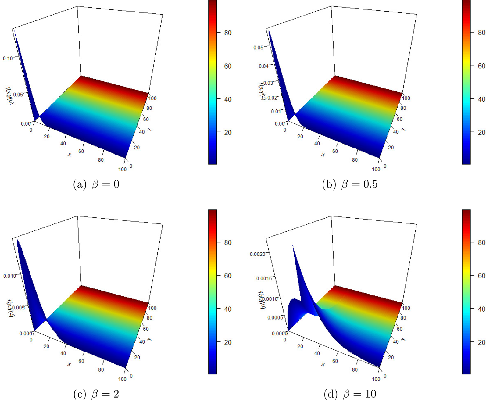
Second, we consider an example with zero-truncated negative-binomial batch arrivals and exponential claim amounts.

As stated in Section 3, zero-truncated negative-binomial batch arrivals may also accommodate both under- and over-dispersed data, while the resulting Poisson-Negative-Binomial counting process is still over-dispersed. Let $r = 5$. When $\alpha = 0.2$, the batch arrivals are under-dispersed, while when $\alpha = 0.5$ or 2, the batch arrivals are over-dispersed. We also consider the single-claim-arrival case for comparison and denote its parameter by $\alpha$ $\downarrow$ 0 as $\alpha = 0$ is not admissible for the negative binomial distribution, and we may then define this case as $p_1=1,$ which in turn will result in the classical compound Poisson model. The c.d.f. of the zero-truncated negative binomial distribution in the four cases for $\alpha$ are plotted in Figure 6. The plot implies that the model whose batch arrivals follow the zero-truncated negative binomial distribution with larger $\alpha$ is more likely to receive a larger number of claims at a time. This means that an insurance company with more business requires a model with a larger $\alpha$.

Figure 6.

C.d.f. of the zero-truncated negative binomial distribution.

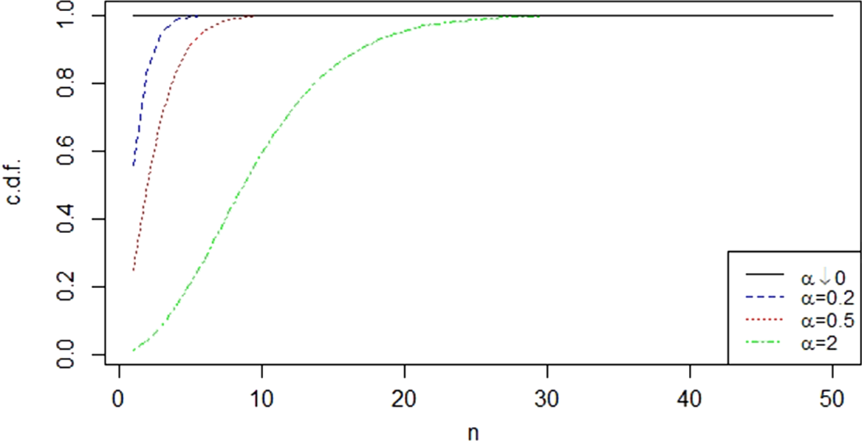
The probability of ultimate ruin for different $\alpha$ is then plotted in Figure 7. It is confirmed in Figure 7 that the probability of ultimate ruin decreases with the increase of the initial surplus and reaches zero when the initial surplus is large enough. Moreover, the approximate values of $u$ for $\psi (u) = 0$ and $5\%$ for four different values of $\alpha$ are summarized in Table 2. Based on the results in the table, for the same level of initial surplus, the larger the $\alpha$, the larger the probability of ruin is. Thus, over-dispersed batch arrivals correspond to a higher risk of ruin as it should be expected. Moreover, Figure 7 stresses further that the possibility of batch-claim arrivals has a significant effect on the probability of ruin and should not be underestimated. Again, the approximate value of $u$ when the probability of ultimate ruin drops to $5\%$ is nearly half of that when the probability of ultimate ruin reaches zero, especially when $\alpha$ is small. This implies that the insurance companies may only require half of the initial surplus needed for avoiding the vast majority of the risk of ruin to maintain a relatively low risk of ruin.

Figure 7.

Probability of ultimate ruin.

Table 2.

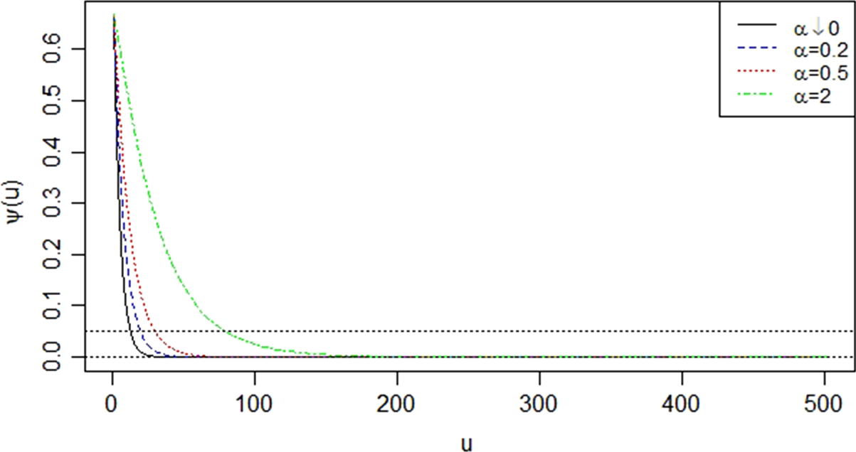
Approximate values of $u$ for which the respective values for $\psi$ are reached for the first time.

The mean and variance of the ruin time are plotted in Figures 8 and 9, respectively. These plots seem to present linear patterns, which contradict Eq. (35) in Li and Sendova [Reference Li and Sendova6]. Obviously, when $\alpha$ $\downarrow$ 0, the mean and the variance of the ruin time are indeed linear functions of the initial surplus. After more careful analysis, we may confirm that when $\alpha >0,$ e.g., when $\alpha = 0.2$, 0.5 or 2, the mean and the variance of the ruin time are not linear. More specifically, the mean of the ruin time seems to be a concave function, which implies that the mean of the ruin time increases slower when the initial surplus is larger. Meanwhile, the variance of the ruin time seems to have a convex shape, which indicates that the variance increases faster as the initial surplus gets larger. We also observe that for the same level of the initial surplus, the model with a higher $\alpha$ corresponds to lower mean and variance of the ruin time. In other words, over-dispersed batch arrivals lead to shorter ruin time. This is another indication that the possibility of batch arrivals should not be underestimated when a model is being built.

Figure 8.

Mean of the ruin time.

Figure 9.

Variance of the ruin time.

Assume that $u=25$. The proper joint density of the surplus before ruin and the deficit at ruin for different $\alpha$ are plotted in Figure 10. We also observe that most often ruin happens when the current surplus drops below the initial surplus. When $\alpha$ is larger, ruin may also occur when the current surplus is larger than the initial surplus. It shows that when the Poisson-Negative-Binomial model is utilized, especially for over-dispersed batch arrivals, ruin happens more dispersedly compared with the no-batch-arrival case ($\alpha$ $\downarrow$ 0).

Figure 10.

Proper joint density of the surplus before ruin and the deficit at ruin for different $\alpha$.

As we can see, the results obtained in the case of zero-truncated geometric batch arrivals are in tune with the results obtained in the case of zero-truncated negative-binomial batch arrivals, which reflects the fact that the zero-truncated geometric distribution is a special case of the zero-truncated negative-binomial distribution.

Third, we consider an example with zero-truncated binomial-batch arrivals and exponential-claim amounts.

As stated in Section 3, the zero-truncated binomial-batch arrivals may only accommodate over-dispersed data, while the resulting Poisson-Binomial counting process is always over-dispersed. Let $l = 5$. When $q = 0.2$, 0.5 or 0.8, the batch arrivals are all over-dispersed. The single-claim arrival case $q$ $\downarrow$ 0 is also considered for comparison. We use $q$ $\downarrow$ 0 this value of $q$ as it as $q = 0$ is not admissible, so we may define it additionally to result in $p_1=1$. The c.d.f. of the zero-truncated binomial distribution in the four cases for $q$ is plotted in Figure 11. The plot indicates that the model whose batch arrivals follow the zero-truncated binomial distribution with larger $q$ is more likely to receive larger number of claims at a time. This means that an insurance company with more business requires a model with a larger $q$.

Figure 11.

C.d.f. of the zero-truncated binomial distribution.

The probability of ultimate ruin for the different values of $q$ is then plotted in Figure 12. This plot verifies that the probability of ultimate ruin decreases with the increase of the initial surplus and reaches zero when the initial surplus is large enough. Namely, the approximate values of $u$ for $\psi (u) = 0$ and $5\%$ for the four different values of $q$ are summarized in Table 3. Hence, we have seen that for the same level of initial surplus, the larger the $q$, the larger the probability of ruin is. Figure 12 implies that batch-claim arrivals under this model do influence the probability of ruin, but the influence might not be that significant compared with the zero-truncated geometric and the negative-binomial batch arrivals cases. In addition, the approximate value of $u$ when the probability of ultimate ruin falls to $5\%$ is approximately half of the initial surplus when the probability of ultimate ruin reaches zero. This means that in order to maintain a relatively low risk of ruin, the insurance companies may only require half of the initial surplus needed for eliminating most of the risk of ruin.

Figure 12.

Probability of ultimate ruin.

Table 3.

Approximate values of $u$ for which the respective values for $\psi$ are reached for the first time.

The mean and variance of the ruin time are plotted in Figures 13 and 14. These plots show approximately linear patterns. Obviously, when $q \downarrow 0$, the mean and the variance of the ruin time are indeed linear functions of the initial surplus. However, when $q\in (0,1),$ e.g., $q = 0.2$, 0.5 or 0.8, empirical analysis shows that the mean and the variance of the ruin time are not linear. To be specific, the mean of the ruin time seems to be concave, which implies that when the initial surplus is larger, the mean of the ruin time increases slower. At the same time, the variance of the ruin time seems to be convex, which indicates that the variance increases faster when the initial surplus is larger. All in all, for the same level of the initial surplus, the model with a higher $q$ corresponds to lower mean and variance of the ruin time.

Figure 13.

Mean of the ruin time.

Figure 14.

Variance of the ruin time.

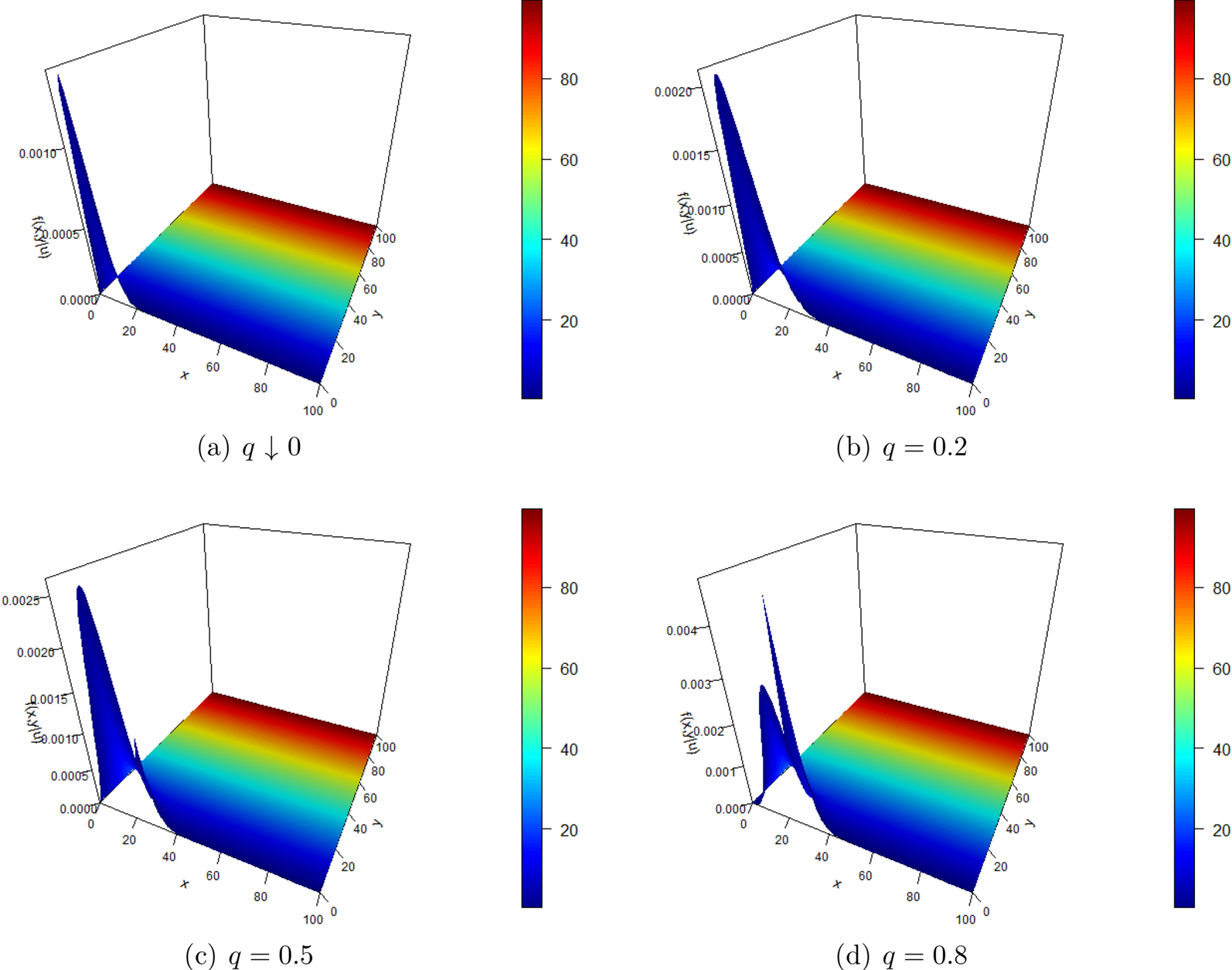
Assume that $u=25$. The proper joint density of the surplus before ruin and the deficit at ruin for different $q$ are plotted in Figure 15. Notice that whenever ruin occurs, it happens with exceedingly high probability that when the current surplus drops below the initial surplus. The value of $q$ has relatively small effect on the distribution of the surplus before ruin and the deficit at ruin. It shows that the Poisson-Binomial model may not yield significant modeling improvements compared with the no-batch-arrival case.

Figure 15.

Proper joint density of the surplus before ruin and the deficit at ruin for different $q$.

4.2. Erlang($k$) claim amounts

This subsection is dedicated to Erlang($k$) claim amounts and we choose $k=3$. For comparison reasons, we will utilize the same parameter values as in the examples with exponential-claim amounts in Subsection 4.1.

Firstly, we consider an example in the case of zero-truncated geometric batch arrivals.

As before, we choose $\beta = 0$, 0.5, 2 and 10. The c.d.f. of the zero-truncated geometric distribution in the four cases for $\beta$ is plotted in Figure 1 in Subsection 4.1.

The probability of ultimate ruin for different $\beta$ is then plotted in Figure 16. As is shown in the plot, the probability of ultimate ruin decreases with the increase of the initial surplus and reaches zero when the initial surplus is large enough. The approximate values of $u$ for $\psi (u) = 0$ and $5\%$ for four different values of $\beta$ are summarized in Table 4. Again, for the same level of initial surplus, the larger $\beta$ is, the larger the probability of ruin is. Compared with the exponential case, the Erlang($k$) case may require a higher level of initial surplus to maintain a low risk of ruin. Meanwhile, we still observe that the approximate value of $u$ when the probability of ultimate ruin falls to $5\%$ is nearly half of that when the probability of ultimate ruin reaches zero, especially when $\beta$ is small.

Figure 16.

Probability of ultimate ruin.

Table 4.

Approximate values of $u$ for which the respective values for $\psi$ are reached for the first time.

The mean and variance of the ruin time are plotted in Figures 17 and 18, respectively. These plots show approximately linear patterns. However, empirical analysis shows that the mean and the variance of the ruin time are not linear functions of the initial surplus. More specially, for all four different values for $\beta$, the mean of the ruin time seems to show a concave shape, while the variance of the ruin time seems to have a convex pattern. We also observe that for the same level of the initial surplus, the model with a higher $\beta$ corresponds to lower mean and variance of the ruin time.

Figure 17.

Mean of the ruin time.

Figure 18.

Variance of the ruin time.

Assume that $u=25$. The proper joint density of the surplus before ruin and the deficit at ruin for different $\beta$ are plotted in Figure 19. Similar to the exponential case, it seems that most frequently, ruin occurs when the current surplus drops below the initial surplus. When $\beta$ is larger, ruin may also happen when the current surplus is larger than the initial surplus. Besides, the joint density comes to a higher peak when $\beta$ is small. It shows that when the Poisson-Geometric model is employed, especially for over-dispersed batch arrivals, ruin happens more dispersedly compared with the no-batch-arrival case. And the effect of ruin being more dispersed is even more significant compared with the exponential-claim-amount case.

Figure 19.

Proper joint density of the surplus before ruin and the deficit at ruin for different $\beta$.

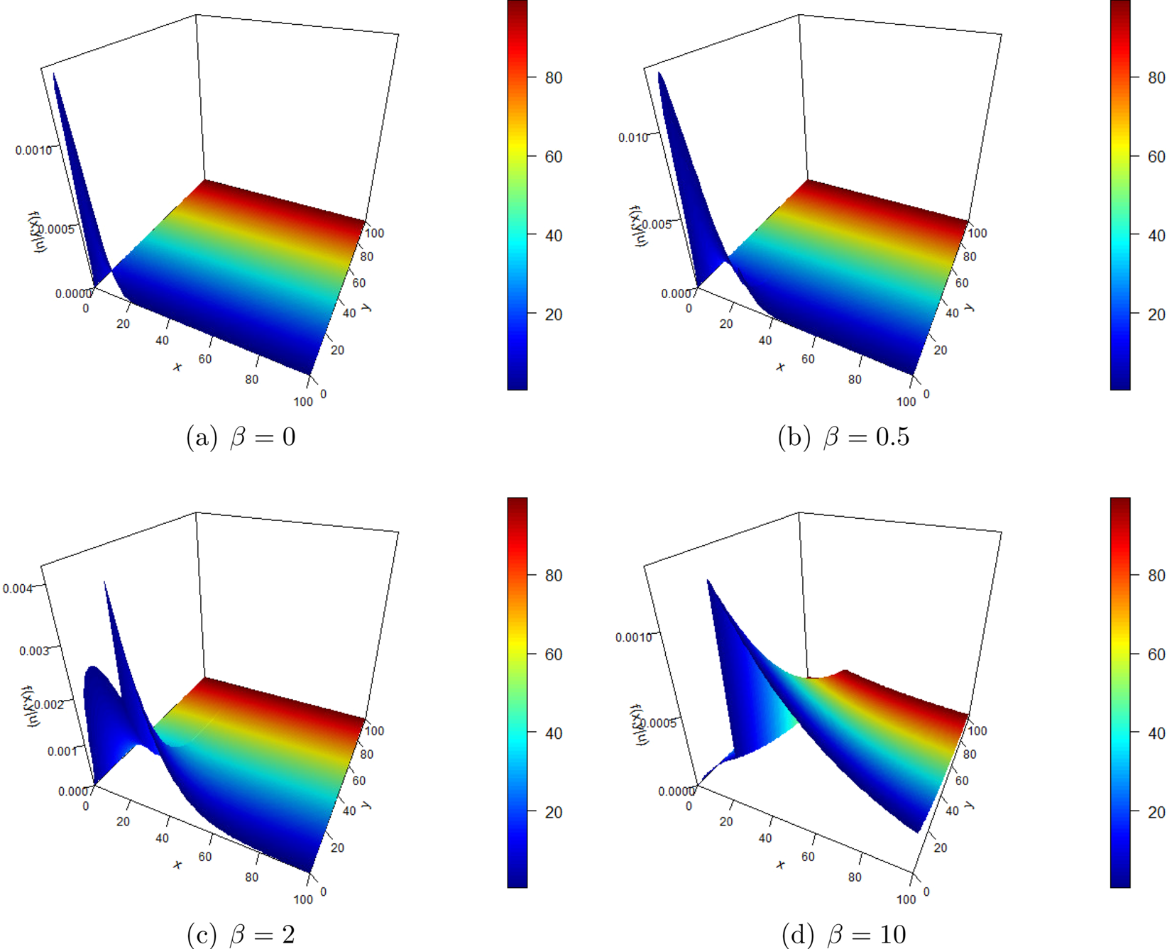
Secondly, we consider an example with zero-truncated negative-binomial batch arrivals.

Again, we assume $\alpha = 0$, 0.2, 0.5 and 2. Recall that we define the case $\alpha$ $\downarrow$ 0 as $p_1 = 1$, since the value of $\alpha = 0$ is not admissible for the negative-binomial distribution. The c.d.f. of the zero-truncated negative-binomial distribution in the four cases for $\alpha$are plotted in Figure 6 in Subsection 4.1.

The probability of ultimate ruin for the different values of $\alpha$ is then plotted in Figure 20. As the plot shows, the probability of ultimate ruin decreases with the increase of the initial surplus and reaches zero when the initial surplus is large enough. Moreover, the approximate values of $u$ for $\psi (u) = 0$ and $5\%$ for four different values of $\alpha$ are summarized in Table 5. For the same level of initial surplus, the larger $\alpha$, the larger the probability of ruin is. Compared with the exponential-claim-amount case, the Erlang($k$)-claim-amount case may require a higher level of initial surplus to maintain a low risk of ruin. And the approximate value of $u$ when the probability of ultimate ruin drops to $5\%$ is nearly half of that when the probability of ultimate ruin reaches zero, especially when $\alpha$ is small.

Figure 20.

Probability of ultimate ruin.

Table 5.

Approximate values of $u$ for which the respective values for $\psi$ are reached for the first time.

The mean and variance of the ruin time are plotted in Figures 21 and 22, respectively. Similar to the exponential case, the mean and the variance of the ruin time seem to have linear patterns, but are not linear functions of the initial surplus. This time, for all four different values for $\alpha$, the mean of the ruin time seems to be concave, while the variance of the ruin time seems to be convex. And again, for the same level of the initial surplus, the model with a higher $\alpha$ corresponds to lower mean and variance of the ruin time.

Figure 21.

Mean of the ruin time.

Figure 22.

Variance of the ruin time.

Thirdly, we consider an example with zero-truncated binomial-batch arrivals. As before, we set $l = 5$ and $q\downarrow 0$, 0.2, 0.5 and 0.8. Again, we define the case $q \downarrow 0$ to result in $p_1 = 1$ as $q = 0$ is not admissible for the binomial distribution. The c.d.f. of the zero-truncated negative-binomial distribution in the four cases for $q$ is plotted in Figure 11 in Subsection 4.1.

The probability of ultimate ruin for the different values of $q$ is then plotted in Figure 20. As is shown in the plot, the probability of ultimate ruin decreases with the increase of the initial surplus and reaches zero when the initial surplus is large enough. That is, the approximate values of $u$ for $\psi (u) = 0$ and $5\%$ for four different values of $q$ are summarized in Table 6. For the same level of initial surplus, the larger $q$, the larger the probability of ruin is. For the Erlang($k$)-claim-amount case, the batch arrivals do not have a significant influence on the probability of ruin either. Once again, the approximate value of $u$ when the probability of ultimate ruin falls to $5\%$ is about half of that when the probability of ultimate ruin reaches zero, especially when $\beta$ is small (Figure 23).

Figure 23.

Probability of ultimate ruin.

Table 6.

Approximate values of $u$ for which the respective values for $\psi$ are reached for the first time.

The mean and variance of the ruin time are plotted in Figures 24 and 25. Similar to the exponential-claim-amount case, the mean and the variance of the ruin time present approximately linear patterns but are not linear functions of the initial surplus. Again, for all four different values for $q$, the mean of the ruin time seems to present a concave pattern, while the variance of the ruin time seems to show a convex shape. We also observe that for the same level of the initial surplus, the model with a higher $q$ corresponds to lower mean and variance of the ruin time.

Figure 24.

Mean of the ruin time.

Figure 25.

Variance of the ruin time.

Assume that $u=25$. The proper joint density of the surplus before ruin and the deficit at ruin for different $q$ are plotted in Figure 26. It seems that most often, ruin happens when the current surplus drops below the initial surplus. There are also instances of ruin occurring when the current surplus is larger than the initial surplus. Therefore, the value of $q$ has small effect on the distribution of the surplus before ruin and the deficit at ruin, but the effect is a little bit more significant compared with the exponential-claim-amount case. In general, the Poisson-Binomial model may not lead to a significant improvement compared with the no-batch-arrival case.

Figure 26.

Proper joint density of the surplus before ruin and the deficit at ruin for different $q$.