


1. Introduction
Dimer models on surfaces are oriented graphs embedded in surfaces which arise from gluing oriented discs along common arrows. They have been studied in different contexts, including statistical mechanics [Reference Temperley and Fisher10], integrable systems [Reference Goncharov and Kenyon6] and mirror symmetry [Reference Bocklandt2]. More recently, dimer models on surfaces with a boundary have been considered; cf. [Reference Baur, King and Marsh1, Reference Franco, Galloni and Mariotti5] in the context of cluster algebras and cluster categories, as they arise as quivers of clusters with frozen variables or as quivers of cluster-tilting objects with projective-injective summands.
For dimer quivers in the disc, Postnikov diagrams provide a convenient way to describe the cluster structure associated with the Grassmannian Gr $(k,n)$
of
$(k,n)$
of $k$
-dimensional subspaces of
$k$
-dimensional subspaces of $\mathbb{C}^n$
. Postnikov diagrams are a collection of
$\mathbb{C}^n$
. Postnikov diagrams are a collection of $n$
oriented curves between the
$n$
oriented curves between the $n$
vertices of the disc, inducing a permutation of the
$n$
vertices of the disc, inducing a permutation of the $n$
vertices. If this permutation sends vertex
$n$
vertices. If this permutation sends vertex $i$
to vertex
$i$
to vertex $i+k$
(reducing modulo
$i+k$
(reducing modulo $n$
), we say it is a
$n$
), we say it is a $(k,n)$
-diagram; these diagrams are used in the description of the cluster algebra structure on the coordinate ring of the Grassmannian [Reference Scott9] or of the cluster-tilting objects in the Grassmannian cluster category [Reference Baur, King and Marsh1]. A natural question is how to generalise these constructions to other surfaces while retaining control of their algebraic properties. The annulus is the first non-simply connected case, and in this setting, it is known that gluing along boundary intervals changes the topology of the ambient surface and turns boundary arrows into internal arrows along the resulting seams [Reference Baur, King and Marsh1].
$(k,n)$
-diagram; these diagrams are used in the description of the cluster algebra structure on the coordinate ring of the Grassmannian [Reference Scott9] or of the cluster-tilting objects in the Grassmannian cluster category [Reference Baur, King and Marsh1]. A natural question is how to generalise these constructions to other surfaces while retaining control of their algebraic properties. The annulus is the first non-simply connected case, and in this setting, it is known that gluing along boundary intervals changes the topology of the ambient surface and turns boundary arrows into internal arrows along the resulting seams [Reference Baur, King and Marsh1].
The first aim of this paper is to introduce a gluing operation for dimer quivers and to describe how the associated dimer and boundary algebras behave under gluing. Proposition5.14 shows that the glued dimer algebra is determined by the components, and Theorem5.16 shows that, under thinness hypotheses, the glued boundary algebra can also be recovered from the components. In particular, Corollary5.17 gives a recursive way to determine the boundary algebra of a Postnikov diagram in the disc.
The second aim is to use this gluing construction to build homogeneous dimer quivers on annuli in the sense that the associated strand diagram induces a permutation of the form $i\mapsto i+k$
along each of the two components of the boundary; we say that such a diagram is of degree
$i\mapsto i+k$
along each of the two components of the boundary; we say that such a diagram is of degree $k$
. With this in mind, we introduce a family of bridge quivers
$k$
. With this in mind, we introduce a family of bridge quivers $\Theta _k$
and glue them to
$\Theta _k$
and glue them to $(k,n)$
-diagrams in the disc. Theorem7.2 shows that the resulting quivers on the annulus correspond to weak Postnikov diagrams of degree
$(k,n)$
-diagrams in the disc. Theorem7.2 shows that the resulting quivers on the annulus correspond to weak Postnikov diagrams of degree $k$
, and Theorem7.14 gives an explicit presentation of the resulting boundary algebra. Our gluing construction can be used to construct dimer quivers on general surfaces from those on “simpler” surfaces. It would be interesting to do this in a way such that the associated (weak) Postnikov diagrams are also homogenous in the above sense, that is, of degree
$k$
, and Theorem7.14 gives an explicit presentation of the resulting boundary algebra. Our gluing construction can be used to construct dimer quivers on general surfaces from those on “simpler” surfaces. It would be interesting to do this in a way such that the associated (weak) Postnikov diagrams are also homogenous in the above sense, that is, of degree $k$
.
$k$
.
The paper is organised as follows. Sections 2 and 3 contain the necessary background on dimer quivers, Postnikov diagrams and their associated algebras. In Section 4, we recall weak Postnikov diagrams on arbitrary surfaces. Section 5 introduces the gluing operation and studies its effect on dimer and boundary algebras. Section 6 introduces the bridge quivers $\Theta _k$
. In Section 7, we use these quivers to construct weak Postnikov diagrams of degree
$\Theta _k$
. In Section 7, we use these quivers to construct weak Postnikov diagrams of degree $k$
on annuli and to determine their boundary algebras.
$k$
on annuli and to determine their boundary algebras.
In particular, we show that the dimer algebras (Definition2.7) obtained through gluing are determined by the components used in the gluing (Proposition5.14). Additionally, when certain consistency conditions are met, we also determine the glued boundary algebra from the components in Theorem5.16. Notably, this allows the boundary algebra associated arbitrary Postnikov diagrams on the disc to be calculated recursively using Corollary5.17. In Section 6, we introduce a family of consistent dimer quivers on the disc, called $k$
-bridges. These will be instrumental in the construction of dimer quivers for the annulus in Section 7. In this final section, we glue bridge quivers with certain homogeneous dimer quivers on the disc, called
$k$
-bridges. These will be instrumental in the construction of dimer quivers for the annulus in Section 7. In this final section, we glue bridge quivers with certain homogeneous dimer quivers on the disc, called $(k,n)$
-diagrams. We prove that the resulting dimer quivers on the annulus correspond to weak Postnikov diagrams of degree
$(k,n)$
-diagrams. We prove that the resulting dimer quivers on the annulus correspond to weak Postnikov diagrams of degree $k$
in Theorem7.14.
$k$
in Theorem7.14.
2. Dimer quivers
A quiver is an oriented graph $Q=(Q_0,Q_1)$
, with a finite vertex set
$Q=(Q_0,Q_1)$
, with a finite vertex set $Q_0$
and a finite set of arrows (oriented edges)
$Q_0$
and a finite set of arrows (oriented edges) $Q_1$
. We denote by
$Q_1$
. We denote by $Q_{cyc}$
the set of oriented cycles in
$Q_{cyc}$
the set of oriented cycles in $Q$
.
$Q$
.
Definition 2.1.
A quiver with faces is a quiver $Q=(Q_0,Q_1)$
together with a set of faces
$Q=(Q_0,Q_1)$
together with a set of faces $Q_2$
and a map
$Q_2$
and a map $\partial \,:\, Q_2 \to Q_{cyc}$
sending a face
$\partial \,:\, Q_2 \to Q_{cyc}$
sending a face $F \in Q_2$
to its boundary
$F \in Q_2$
to its boundary $\partial F \in Q_{cyc}$
.
$\partial F \in Q_{cyc}$
.
We consider a special class of quivers with faces obtained from gluing a collection of oriented cycles along arrows in a consistent way. They were first formalised in [Reference Baur, King and Marsh1] as dimer models with a boundary. We will call them dimer quivers.
We first recall the notion of the incidence graph of a vertex of $Q$
: For vertex
$Q$
: For vertex $i \in Q_0$
of the quiver
$i \in Q_0$
of the quiver $Q$
, the incidence graph of
$Q$
, the incidence graph of $Q$
at
$Q$
at $i$
has as vertices the set of arrows incident with
$i$
has as vertices the set of arrows incident with $i$
and contains an edge between vertices
$i$
and contains an edge between vertices $v_{\alpha }$
and
$v_{\alpha }$
and $v_{\beta }$
if the path
$v_{\beta }$
if the path
 \begin{align*} \bullet \stackrel {\alpha }{\longrightarrow } i \stackrel {\beta }{\longrightarrow }\bullet \end{align*}
is part of the boundary $\partial F$
of a face
$\partial F$
of a face $F\in Q_2$
.
$F\in Q_2$
.
If $\alpha \in Q_1$
, the face multiplicity of
$\alpha \in Q_1$
, the face multiplicity of $\alpha$
is the number of faces such that
$\alpha$
is the number of faces such that $\alpha$
belongs to their boundary.
$\alpha$
belongs to their boundary.
Definition 2.2.
A dimer quiver is a quiver with faces $(Q_0,Q_1,Q_2)$
where
$(Q_0,Q_1,Q_2)$
where $Q_2$
can be expressed as the disjoint union of two sets
$Q_2$
can be expressed as the disjoint union of two sets $Q_2^+$
and
$Q_2^+$
and $Q_2^-$
and which satisfies the additional properties:
$Q_2^-$
and which satisfies the additional properties:
-
(1) $Q$
has no loops.
$Q$
has no loops.
-
(2) Every arrow
$\alpha$
in
$Q_1$
appears with face multiplicity one or two. In the latter case, if
$F_1$
and
$F_2$
are the two faces
$F_1,F_2$
, such that
$\alpha \in \partial F_i$
for
$i=1,2$
, then
$F_1\in Q_2^+$
and
$F_2\in Q_2^-$
(or vice versa).
-
(3) The incidence graph of every vertex of
$Q_0$
is (non-empty and) connected.


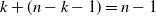
Notice that a dimer quiver partitions the set of faces $Q_2$
according to the orientation of their boundary cycles in a way that the boundaries of any two adjacent faces have opposite orientations. See Figure 1 for an illustration.
$Q_2$
according to the orientation of their boundary cycles in a way that the boundaries of any two adjacent faces have opposite orientations. See Figure 1 for an illustration.
Remark 2.3. Dimer quivers are the dual graphs to certain well-studied bipartite graphs on surfaces called dimer models (see [Reference Broomhead3, Reference Hanany and Kennaway7, Reference Temperley and Fisher10], e.g.).
If $\alpha$
has face multiplicity one in the dimer quiver
$\alpha$
has face multiplicity one in the dimer quiver $Q$
, we call
$Q$
, we call $\alpha$
a boundary arrow; otherwise,
$\alpha$
a boundary arrow; otherwise, $\alpha$
is an internal arrow. A vertex
$\alpha$
is an internal arrow. A vertex $i\in Q_0$
is a boundary vertex if it is incident with a boundary arrow. Otherwise,
$i\in Q_0$
is a boundary vertex if it is incident with a boundary arrow. Otherwise, $i$
is called internal.
$i$
is called internal.
Example 2.4.
Figure
1
shows an example of a dimer quiver with six faces. The partition of $Q_2$
is indicated by the shading:
$Q_2$
is indicated by the shading:
 \begin{align*} Q_2^+ =\{F_1,F_3,F_5\} \quad \mbox{and} \quad Q_2^- = \{F_2,F_4, F_6\}. \end{align*}
A dimer quiver with six faces.

Remark 2.5.
Given a dimer quiver $Q$
, we can form a topological space
$Q$
, we can form a topological space $\Sigma _Q$
by gluing the arrows bounding each face as directed by their orientation. The resulting space
$\Sigma _Q$
by gluing the arrows bounding each face as directed by their orientation. The resulting space $\Sigma _Q$
is an oriented surface with boundary, where the faces in
$\Sigma _Q$
is an oriented surface with boundary, where the faces in $Q_2^+, Q_2^-$
can be declared to have positive and negative orientations, respectively. The quiver
$Q_2^+, Q_2^-$
can be declared to have positive and negative orientations, respectively. The quiver $Q$
is said to be a dimer quiver in a disc, if
$Q$
is said to be a dimer quiver in a disc, if $\Sigma _Q$
is homeomorphic to a disc.
$\Sigma _Q$
is homeomorphic to a disc.
A path $p$
in a quiver
$p$
in a quiver $Q$
is a composition of arrows
$Q$
is a composition of arrows $p=\alpha _1 \alpha _2\cdots \alpha _s$
such that the endpoint of
$p=\alpha _1 \alpha _2\cdots \alpha _s$
such that the endpoint of $\alpha _i$
is equal to the starting point of
$\alpha _i$
is equal to the starting point of $\alpha _{i+1}$
for
$\alpha _{i+1}$
for $i=1,\ldots , s-1$
(writing the composition from left to right). We allow paths of length
$i=1,\ldots , s-1$
(writing the composition from left to right). We allow paths of length $0$
, that is, paths starting and ending at a vertex, without using any arrows. Such a path is called a trivial path. To any quiver
$0$
, that is, paths starting and ending at a vertex, without using any arrows. Such a path is called a trivial path. To any quiver $Q$
, one can associate an algebra over
$Q$
, one can associate an algebra over $\mathbb{C}$
, the so-called path algebra
$\mathbb{C}$
, the so-called path algebra $\mathbb{C}Q$
of
$\mathbb{C}Q$
of $Q$
: it has as a basis the set of all paths of
$Q$
: it has as a basis the set of all paths of $Q$
, including the trivial ones, with multiplication given by the concatenation of paths. Note that since the dimer quivers we consider contain-oriented cycles, the associated path algebras are infinitely dimensional.
$Q$
, including the trivial ones, with multiplication given by the concatenation of paths. Note that since the dimer quivers we consider contain-oriented cycles, the associated path algebras are infinitely dimensional.
For any oriented face $F \in Q_2$
, the element
$F \in Q_2$
, the element $\partial F$
determines a cycle in
$\partial F$
determines a cycle in $Q$
, and so the set of all cycles defines an element
$Q$
, and so the set of all cycles defines an element
 \begin{align*} W_{Q}=\sum _{F \in Q_{2}^{+}} \partial F-\sum _{F \in Q_{2}^{-}} \partial F \end{align*}
in $\mathbb{C}Q_{cyc}$
called the potential of
$\mathbb{C}Q_{cyc}$
called the potential of $Q$
.
$Q$
.
Internal arrows impose relations on the path algebra, given by the so-called cyclic derivatives of the potential:
Definition 2.6.
Let $\alpha$
be an internal arrow of
$\alpha$
be an internal arrow of $Q$
, and let
$Q$
, and let $\alpha \beta _1\cdots \beta _s=\partial F_1\in Q_{cyc}$
and
$\alpha \beta _1\cdots \beta _s=\partial F_1\in Q_{cyc}$
and $\alpha \gamma _1\cdots \gamma _t=\partial F_2\in Q_{cyc}$
be the two boundary cycles of the faces in
$\alpha \gamma _1\cdots \gamma _t=\partial F_2\in Q_{cyc}$
be the two boundary cycles of the faces in $Q_2$
containing
$Q_2$
containing $\alpha$
, with
$\alpha$
, with $F_1\in Q_2^+$
and
$F_1\in Q_2^+$
and $F_2\in Q_2^-$
. Let
$F_2\in Q_2^-$
. Let $p_{F_1}\,:\!=\,\beta _1\cdots \beta _s$
and
$p_{F_1}\,:\!=\,\beta _1\cdots \beta _s$
and $p_{F_2}\,:\!=\,\gamma _1\cdots \gamma _t$
denote the complements of
$p_{F_2}\,:\!=\,\gamma _1\cdots \gamma _t$
denote the complements of $\alpha$
in
$\alpha$
in $\partial F_1$
and
$\partial F_1$
and $\partial F_2$
, respectively. Then the cyclic derivative of
$\partial F_2$
, respectively. Then the cyclic derivative of $W_Q$
with respect to
$W_Q$
with respect to $\alpha$
is defined by
$\alpha$
is defined by
 \begin{align*} \partial _{\alpha }(W_Q)=p_{F_1}-p_{F_2}. \end{align*}
The potential $W_Q$
determines an ideal of relations. We write
$W_Q$
determines an ideal of relations. We write
 \begin{align*} I_W\,:\!=\,\langle \partial _{\alpha }(W_Q)\,:\, \alpha \in Q_1,\quad \alpha \text{ internal}\rangle \end{align*}
for the ideal of $\mathbb C Q$
generated by the cyclic derivatives with respect to internal arrows.
$\mathbb C Q$
generated by the cyclic derivatives with respect to internal arrows.
Definition 2.7.
Let $Q$
be a dimer quiver; the dimer algebra
$Q$
be a dimer quiver; the dimer algebra $A_Q$
is defined to be the quotient of the path algebra by the relations arising from internal arrows
$A_Q$
is defined to be the quotient of the path algebra by the relations arising from internal arrows $\alpha \in Q_1$
:
$\alpha \in Q_1$
:
 \begin{align*} A_Q\,:\!=\,\mathbb{C}Q/I. \end{align*}
Note that while many paths get identified in $A_Q$
, the dimer algebra is still infinite dimensional in general. Indeed, by Lemma2.8 below, the element
$A_Q$
, the dimer algebra is still infinite dimensional in general. Indeed, by Lemma2.8 below, the element $t=\sum _{i\in Q_0}u_i$
generates a polynomial subalgebra
$t=\sum _{i\in Q_0}u_i$
generates a polynomial subalgebra $\mathbb C[t]\subseteq Z(A_Q)$
.
$\mathbb C[t]\subseteq Z(A_Q)$
.
Any boundary cycle of a face is called a unit cycle. As a consequence of the definition, for any vertex $I\in Q_0$
, the different unit cycles going through a vertex
$I\in Q_0$
, the different unit cycles going through a vertex $i$
are all equivalent in
$i$
are all equivalent in $A_Q$
. We write
$A_Q$
. We write $u_i$
to denote the corresponding element in
$u_i$
to denote the corresponding element in $A_Q$
.
$A_Q$
.
Lemma 2.8.
Let $t$
be the element of
$t$
be the element of $A_Q$
given by
$A_Q$
given by $t\,:\!=\, \sum _{i \in Q_0}u_i$
, then
$t\,:\!=\, \sum _{i \in Q_0}u_i$
, then $\mathbb{C}[t] \subseteq Z(A_Q)$
, where
$\mathbb{C}[t] \subseteq Z(A_Q)$
, where $Z(A_Q)$
denotes the centre of
$Z(A_Q)$
denotes the centre of $A_Q$
.
$A_Q$
.
Proof.
It suffices to show that $t$
commutes with any arrow
$t$
commutes with any arrow $\alpha \in Q_1$
. Suppose
$\alpha \in Q_1$
. Suppose $\alpha$
is an arrow starting at vertex
$\alpha$
is an arrow starting at vertex $i$
and terminating at vertex
$i$
and terminating at vertex $j$
. Then
$j$
. Then $t\alpha =u_i\alpha$
and
$t\alpha =u_i\alpha$
and $\alpha t=\alpha u_j$
; therefore, we only have to show
$\alpha t=\alpha u_j$
; therefore, we only have to show $u_i\alpha =\alpha u_j$
. Let
$u_i\alpha =\alpha u_j$
. Let $F \in Q_2$
be a face whose boundary is given by
$F \in Q_2$
be a face whose boundary is given by $\partial F =\alpha p_F$
. As
$\partial F =\alpha p_F$
. As $\alpha p_F$
is a unit cycle at
$\alpha p_F$
is a unit cycle at $i$
, we have
$i$
, we have $u_i\alpha = \alpha p_F \alpha$
. Similarly,
$u_i\alpha = \alpha p_F \alpha$
. Similarly, $p_F \alpha$
is a unit cycle at
$p_F \alpha$
is a unit cycle at $j$
, and so
$j$
, and so $\alpha p_F \alpha = \alpha u_j$
.
$\alpha p_F \alpha = \alpha u_j$
.
Definition 2.9.
Let $Q$
be a dimer quiver and
$Q$
be a dimer quiver and $A_Q$
its dimer algebra. Let
$A_Q$
its dimer algebra. Let $e_1,\ldots , e_n$
be the idempotent elements of
$e_1,\ldots , e_n$
be the idempotent elements of $A_Q$
corresponding to the trivial paths at the boundary vertices of
$A_Q$
corresponding to the trivial paths at the boundary vertices of $Q$
and set
$Q$
and set $e=\sum _{i=1}^n e_i$
. Then the boundary algebra of
$e=\sum _{i=1}^n e_i$
. Then the boundary algebra of $Q$
is defined to be the algebra given by:
$Q$
is defined to be the algebra given by:
 \begin{align*} B_Q=eA_Qe. \end{align*}
This is often called the ‘idempotent subalgebra of $A_Q$
’ as we pre- and postcompose all paths with the idempotent element
$A_Q$
’ as we pre- and postcompose all paths with the idempotent element $e$
of
$e$
of $A_Q$
.
$A_Q$
.
Note that the boundary algebra of a dimer quiver is also infinite dimensional in general.
3. Postnikov diagrams
In this section, we consider certain diagrams in the disc: the surface $\Sigma$
is a disc with
$\Sigma$
is a disc with $n$
marked points on the boundary. These diagrams correspond to dimer quivers in the disc that exhibit global properties which will later be used to determine the corresponding boundary algebra.
$n$
marked points on the boundary. These diagrams correspond to dimer quivers in the disc that exhibit global properties which will later be used to determine the corresponding boundary algebra.
Definition 3.1. A Postnikov diagram (in the disc) consists of a collection of oriented curves (strands) in the disc with marked points on its boundary, where each marked point is the source of exactly one strand and the target of exactly one strand. The curves are considered up to isotopy, fixing endpoints. The diagram must satisfy the following axioms.
-
(1) There are finitely many intersections, and each intersection is a transversal of order two.
-
(2) Following a fixed strand, the strands that cross it must alternate between crossing from the left and crossing from the right.
-
(3) Strands have no self-intersections.
-
(4) If two strands cross at distinct points, the corresponding bounded region forms an oriented disc.
The label of a strand is the number $i$
of the marked point where it starts.
$i$
of the marked point where it starts.
It is clear from the definition that a Postnikov diagram determines a permutation of the boundary vertices by $ i \mapsto j$
if the strand starting at vertex
$ i \mapsto j$
if the strand starting at vertex $i$
terminates at vertex
$i$
terminates at vertex $j$
. We call this the strand permutation
$j$
. We call this the strand permutation $\pi _D$
. Postnikov diagrams whose strand permutation takes the form
$\pi _D$
. Postnikov diagrams whose strand permutation takes the form $i \mapsto i+k \ (mod \ n)$
are of particular interest as they describe a cluster in the homogeneous coordinate ring of the Grassmannian Gr
$i \mapsto i+k \ (mod \ n)$
are of particular interest as they describe a cluster in the homogeneous coordinate ring of the Grassmannian Gr $(k,n)$
[Reference Temperley and Fisher10, Theorem 3]. We refer to such a diagram as a
$(k,n)$
[Reference Temperley and Fisher10, Theorem 3]. We refer to such a diagram as a $(k,n)$
-diagram. Note that such diagrams always exist: in the paper mentioned above, Scott gave an explicit construction of a
$(k,n)$
-diagram. Note that such diagrams always exist: in the paper mentioned above, Scott gave an explicit construction of a $(k,n)$
-diagram for every
$(k,n)$
-diagram for every $k\lt n$
.
$k\lt n$
.
Example 3.2.
The following is an example of a $(3,5)$
-diagram. The starting and endpoints of the strands are indicated by grey circles.
$(3,5)$
-diagram. The starting and endpoints of the strands are indicated by grey circles.

Two diagrams are said to be equivalent if one can be obtained from the other through a sequence of local twisting or untwisting moves, which are illustrated in the following diagram. The lower diagram represents the boundary case, the boundary indicated on the left.
Local twisting and untwisting moves.

We call a Postnikov diagram reduced if it may not be simplified via untwisting moves (moving left to right in Figure 2). The diagram in Example3.2 is a reduced Postnikov diagram.
Each diagram divides the interior of the disc into regions, which are the connected regions in the complement of the union of all strands. In the definition of a Postnikov diagram, we required that strands must alternate between crossing from left to right and right to left when following a particular strand. As a consequence, the interior regions can be classified as either:
-
(1) alternating if the strands forming its boundary alternate in orientation, or
-
(2) oriented if the strands are all oriented in the same direction (all clockwise or all anticlockwise).
We associate a label with each alternating region obtained from the Postnikov diagram. These labels are subsets of $[n]=\{1,2,\ldots , n\}$
given by the strands: each strand divides the disc into a left and right region with respect to the strand orientation. This allows us to attach labels to the alternating regions: an alternating region is labelled by
$[n]=\{1,2,\ldots , n\}$
given by the strands: each strand divides the disc into a left and right region with respect to the strand orientation. This allows us to attach labels to the alternating regions: an alternating region is labelled by $i \in [n]$
if the strand starting at
$i \in [n]$
if the strand starting at $i$
keeps the given region on its left.
$i$
keeps the given region on its left.
Example 3.3.
The Postnikov diagram from Example
3.2
has six oriented regions (shaded in grey on the left of Figure
3
) and seven alternating regions, with labels as shown in both pictures. One can see that labels of the alternating regions on the boundary are of the form $i,i+1,i+2$
modulo
$i,i+1,i+2$
modulo $n$
, for
$n$
, for $n=5$
.
$n=5$
.
Postnikov diagram with its labels (left) and with the quiver (right).

We want to associate with every Postnikov diagram a dimer quiver. Its vertices are given by the alternating regions. The arrows arise from crossings: to each intersection point between strands of alternating regions, we associate an arrow between the corresponding vertices, with the direction described in the following diagram in Figure 4. The figure on the right represents the case where both regions are on the boundary.
Associating arrows to intersections of strands.

Definition 3.4.
The quiver $Q_D$
associated with a Postnikov diagram
$Q_D$
associated with a Postnikov diagram $D$
has a vertex set
$D$
has a vertex set $Q_0$
given by the alternating regions. The arrows are given by the intersection points of strands between alternating regions, with orientation as above.
$Q_0$
given by the alternating regions. The arrows are given by the intersection points of strands between alternating regions, with orientation as above.
Notice that we allow arrows between boundary vertices.
Example 3.5.
The quiver $Q_D$
obtained from the Postnikov diagram of Example
3.2
recovers the dimer quiver from Figure 2.4. The quiver
$Q_D$
obtained from the Postnikov diagram of Example
3.2
recovers the dimer quiver from Figure 2.4. The quiver $Q_D$
is shown on the right of Figure
3
. It is drawn on top of the Postnikov diagram, using solid lines, with the vertices corresponding to the alternating regions in
$Q_D$
is shown on the right of Figure
3
. It is drawn on top of the Postnikov diagram, using solid lines, with the vertices corresponding to the alternating regions in $D$
.
$D$
.
We have seen how a Postnikov diagram gives rise to a quiver $Q_D$
. In fact,
$Q_D$
. In fact, $Q_D$
is a dimer quiver in the disc. See [Reference Baur, King and Marsh1, Section 2] for more details.
$Q_D$
is a dimer quiver in the disc. See [Reference Baur, King and Marsh1, Section 2] for more details.
The Postnikov diagram $D$
can be recovered from
$D$
can be recovered from $Q_D$
by taking its strands to be the collection of zig–zag paths of the dimer model [Reference Goncharov and Kenyon6], as we recall here.
$Q_D$
by taking its strands to be the collection of zig–zag paths of the dimer model [Reference Goncharov and Kenyon6], as we recall here.
Definition 3.6.
Let $Q$
be a dimer quiver in the disc, with
$Q$
be a dimer quiver in the disc, with $n$
vertices on the boundary. We draw two short crossing-oriented segments on every arrow of
$n$
vertices on the boundary. We draw two short crossing-oriented segments on every arrow of $Q$
, in the orientation shown on the left and in the middle of Figure
5
. Inside each face, we connect each segment to the next one encountered when moving around the face according to its orientation. In this way we obtain
$Q$
, in the orientation shown on the left and in the middle of Figure
5
. Inside each face, we connect each segment to the next one encountered when moving around the face according to its orientation. In this way we obtain $n$
oriented curves starting and ending at the boundary of the disc, as on the right of the figure. We write
$n$
oriented curves starting and ending at the boundary of the disc, as on the right of the figure. We write $D_Q$
for the resulting diagram. It is sometimes called the diagram of zig–zag paths in
$D_Q$
for the resulting diagram. It is sometimes called the diagram of zig–zag paths in $Q$
.
$Q$
.
In Section 4, we will lift this correspondence to the more general set-up of dimer quivers on arbitrary surfaces and of so-called ‘weak strand diagrams’.
Associating a strand diagram to a dimer quiver.

The weights on the arrows of a dimer quiver.

Definition 3.7 (Reference Baur, King and Marsh1, Section 4). For any arrow $\alpha :I\rightarrow J$
in
$\alpha :I\rightarrow J$
in $Q_1(D)$
, let
$Q_1(D)$
, let $c$
be the label of the strand crossing
$c$
be the label of the strand crossing $\alpha$
from right to left and let
$\alpha$
from right to left and let $d$
be the label of the strand crossing
$d$
be the label of the strand crossing $\alpha$
from left to right, when looking in the direction of
$\alpha$
from left to right, when looking in the direction of $\alpha$
. In other words,
$\alpha$
. In other words, $J=I\setminus \{c\} \cup \{d\}$
. The weight of
$J=I\setminus \{c\} \cup \{d\}$
. The weight of $\alpha$
is then defined to be the cyclic interval from
$\alpha$
is then defined to be the cyclic interval from $c$
to
$c$
to $d$
in
$d$
in $\left [n\right ]$
 \begin{align*} w_\alpha =[c, d). \end{align*}
The weight of a path $p=\alpha _1\cdots \alpha _r$
in
$p=\alpha _1\cdots \alpha _r$
in $Q_D$
is the multiset union of the weights of the arrows in the path; equivalently, it is the sum of the indicator functions of the intervals
$Q_D$
is the multiset union of the weights of the arrows in the path; equivalently, it is the sum of the indicator functions of the intervals $w_{\alpha _1},\ldots ,w_{\alpha _r}$
. We write
$w_{\alpha _1},\ldots ,w_{\alpha _r}$
. We write $\operatorname {supp}(w_p)\subseteq [n]$
for its support. A path is called sincere if
$\operatorname {supp}(w_p)\subseteq [n]$
for its support. A path is called sincere if $\operatorname {supp}(w_p)=[n]$
and insincere otherwise.
$\operatorname {supp}(w_p)=[n]$
and insincere otherwise.
Example 3.8.
To determine the weight of the arrow $\{1,3,5\}\to \{2,3,5\}$
of the quiver from Figure
6
, observe that
$\{1,3,5\}\to \{2,3,5\}$
of the quiver from Figure
6
, observe that $c=1$
and
$c=1$
and $d=2$
. So the weight is
$d=2$
. So the weight is $[1,2)=\{1\}$
. The weights of all arrows of that dimer quiver are shown in Figure
6
. Any arrow is an insincere path. However, as one can check, any unit cycle is a sincere path. The path from
$[1,2)=\{1\}$
. The weights of all arrows of that dimer quiver are shown in Figure
6
. Any arrow is an insincere path. However, as one can check, any unit cycle is a sincere path. The path from $\{3,4,5\}$
to
$\{3,4,5\}$
to $\{1,2,5\}$
via
$\{1,2,5\}$
via $\{1,3,5\}$
and
$\{1,3,5\}$
and $\{1,4,5\}$
has
$\{1,4,5\}$
has $4$
and
$4$
and $5$
with multiplicity two in its weight. It is insincere, since
$5$
with multiplicity two in its weight. It is insincere, since $2$
does not lie in the support.
$2$
does not lie in the support.
Definition 3.9.
A dimer algebra $A_Q$
is called thin if for any pair of vertices
$A_Q$
is called thin if for any pair of vertices $a,b \in Q$
, there is a path
$a,b \in Q$
, there is a path $h\in e_a A_{Q}e_b$
such that
$h\in e_a A_{Q}e_b$
such that $e_a A_{Q}e_b = \mathbb{C}[[t]]h$
. In other words, there is a path
$e_a A_{Q}e_b = \mathbb{C}[[t]]h$
. In other words, there is a path $h\,:\,a \to b$
such that for any path
$h\,:\,a \to b$
such that for any path $g: a \to b$
in
$g: a \to b$
in $A_Q$
, one has
$A_Q$
, one has $g=ht^m$
for some
$g=ht^m$
for some $m\ge 0$
. Such a path will be called minimal.
$m\ge 0$
. Such a path will be called minimal.
Remark 3.10.
For a Postnikov diagram $D$
in the disc, insincere paths in
$D$
in the disc, insincere paths in $A_{Q_D}$
are minimal, cf. [BKM16, Corollary 9.4]. We will use this in the proof of Lemma
3.14
(2).
$A_{Q_D}$
are minimal, cf. [BKM16, Corollary 9.4]. We will use this in the proof of Lemma
3.14
(2).
The following two results on the thinness of dimer algebras will be useful when working with the dimer algebras of Postnikov diagrams.
Proposition 3.11 (Reference Pressland8, Proposition 2.11). Let $D$
be a Postnikov diagram in the disc. If the associated quiver
$D$
be a Postnikov diagram in the disc. If the associated quiver $Q_D$
is connected, then
$Q_D$
is connected, then $A_{Q_D}$
is thin.
$A_{Q_D}$
is thin.
Lemma 3.12 (Reference Pressland8, Lemma 2.13). Let $Q$
be a connected dimer quiver such that
$Q$
be a connected dimer quiver such that $A_Q$
is thin. If
$A_Q$
is thin. If $g: a \to b$
and
$g: a \to b$
and $h: b \to c$
are paths in
$h: b \to c$
are paths in $Q$
such that the composition
$Q$
such that the composition $gh$
is minimal, then both
$gh$
is minimal, then both $g$
and
$g$
and $h$
are minimal.
$h$
are minimal.
We now introduce some notation which will be useful when describing paths between boundary vertices.
Notation 3.13.
Let $D$
be a
$D$
be a $(k,n)$
-diagram in the disc, and let
$(k,n)$
-diagram in the disc, and let $\alpha$
be a boundary arrow in
$\alpha$
be a boundary arrow in $Q_D$
. As each boundary arrow
$Q_D$
. As each boundary arrow $\alpha$
in a dimer quiver
$\alpha$
in a dimer quiver $Q$
belongs to precisely one face
$Q$
belongs to precisely one face $F_\alpha \in Q_2$
, we can uniquely refer to the complement
$F_\alpha \in Q_2$
, we can uniquely refer to the complement $\widehat {\alpha }$
of
$\widehat {\alpha }$
of $\alpha$
around
$\alpha$
around $F_\alpha$
in the dimer algebra
$F_\alpha$
in the dimer algebra $A_Q$
(i.e.,
$A_Q$
(i.e., $\alpha \widehat {\alpha }=\partial F_\alpha$
).
$\alpha \widehat {\alpha }=\partial F_\alpha$
).
For each $i\in [n]$
, we define paths
$i\in [n]$
, we define paths $u_i\,:\,i\to i+1$
and
$u_i\,:\,i\to i+1$
and $v_i\,:\,i+1\to i$
as follows: let
$v_i\,:\,i+1\to i$
as follows: let $\alpha$
be the boundary arrow between
$\alpha$
be the boundary arrow between $i$
and
$i$
and $i+1$
. If
$i+1$
. If $\alpha$
is oriented clockwise (that is, going from
$\alpha$
is oriented clockwise (that is, going from $i$
to
$i$
to $i+1$
, we set
$i+1$
, we set $u_i$
to be this boundary arrow. If
$u_i$
to be this boundary arrow. If $\alpha$
is oriented anticlockwise (i.e.
$\alpha$
is oriented anticlockwise (i.e. $i+1\to i$
), we set
$i+1\to i$
), we set $u_i$
to be
$u_i$
to be $\hat \alpha$
. Then
$\hat \alpha$
. Then $v_i\,:\,i+1\to i$
is defined to be the complement of
$v_i\,:\,i+1\to i$
is defined to be the complement of $u_i$
in the unit cycle at vertex
$u_i$
in the unit cycle at vertex $i$
. Figure
7
gives an illustration of the paths
$i$
. Figure
7
gives an illustration of the paths $u_i$
and
$u_i$
and $v_i$
on a dimer quiver.
$v_i$
on a dimer quiver.
Take $m \in [n]$
and
$m \in [n]$
and $h \geq 0$
. Going forward, we will use the following shorthand for composing
$h \geq 0$
. Going forward, we will use the following shorthand for composing $h$
consecutive
$h$
consecutive $u_i$
’s (
$u_i$
’s ( $v_i$
’s) starting at the vertex
$v_i$
’s) starting at the vertex $m$
on the boundary of
$m$
on the boundary of $Q$
:
$Q$
:
-
•
$u^h_m\,:\!=\, u_{m}u_{m+1}..u_{m+h-1}\,:\, m \to m+h$
-
•
$v^h_m\,:\!=\, v_{m-1}v_{m-2}\ldots v_{m-h}\,:\, m \to m-h$


where addition and subtraction in the indices are done modulo $[n]$
. When the starting point is clear, we will drop the index
$[n]$
. When the starting point is clear, we will drop the index $m$
from the notation. In particular, in Lemma
3.14
(2), the path
$m$
from the notation. In particular, in Lemma
3.14
(2), the path $u^h$
is
$u^h$
is $u^h_a$
, starting at
$u^h_a$
, starting at $a$
and ending at
$a$
and ending at $b\equiv a+h$
and
$b\equiv a+h$
and $v^{h^{\prime}}$
stands for a path starting at
$v^{h^{\prime}}$
stands for a path starting at $a$
and ending at
$a$
and ending at $b\equiv a-h^{\prime}$
.
$b\equiv a-h^{\prime}$
.
Lemma 3.14.
Let $D$
be a
$D$
be a $(k,n)$
-diagram in the disc. The paths defined above satisfy:
$(k,n)$
-diagram in the disc. The paths defined above satisfy:
-
(1)
$v^k_m = u^{n-k}_m$
in
$A_{Q_D}$
for any
$m\in [n]$
. -
(2) For any pair of boundary vertices
$a,b$
in
$Q_D$
, a minimal path from
$a$
to
$b$
in
$A_{Q_D}$
is either
$u_a^h$
or
$v_a^{h^{\prime}}$
, where
$0\le h,h^{\prime}\le n$
,
$b\equiv a+h\equiv a-h^{\prime} \pmod n$
, and
$h+h^{\prime}=n$
.


Paths $u_i$
(in blue) and
$u_i$
(in blue) and $v_i$
(in red).
$v_i$
(in red).

To obtain this result, one can explicitly determine the image of arrows under the inverse of the isomorphism given in [Reference Baur, King and Marsh1, Theorem 11.2] or by analysis of perfect matching modules [Claim 3.4, [Reference Canakci, King and Pressland4]]. However, we provide a direct argument by associating weights to the arrows in $Q_D$
.
$Q_D$
.
Proof of Lemma
3.14. (1) The vertices of $Q_D$
arise from
$Q_D$
arise from $k$
-subsets. For
$k$
-subsets. For $a\in [n]$
, we will write
$a\in [n]$
, we will write $I_a$
for the
$I_a$
for the $k$
-subset
$k$
-subset $\{a,a+1,\ldots , a+k-1\}$
. Adjacent boundary vertices in
$\{a,a+1,\ldots , a+k-1\}$
. Adjacent boundary vertices in $D$
are assigned the
$D$
are assigned the $k$
-element subsets
$k$
-element subsets $I_a$
and
$I_a$
and $I_{a+1}$
of
$I_{a+1}$
of $[n]$
for some
$[n]$
for some $a\in [n]$
. If the boundary arrow between them is oriented clockwise, then
$a\in [n]$
. If the boundary arrow between them is oriented clockwise, then $u_a$
is that arrow and has support
$u_a$
is that arrow and has support $[a,a+k)$
. If the boundary arrow is oriented anticlockwise, then it has support
$[a,a+k)$
. If the boundary arrow is oriented anticlockwise, then it has support $[a+k,a)$
while the unit cycle through it is sincere; hence, its complement
$[a+k,a)$
while the unit cycle through it is sincere; hence, its complement $u_a$
has support
$u_a$
has support $[a,a+k)$
. Similarly, every path
$[a,a+k)$
. Similarly, every path $v\,:\,I_{a+1}\to I_a$
has support
$v\,:\,I_{a+1}\to I_a$
has support $[a+k,a)$
. It is clear that the weight of each path
$[a+k,a)$
. It is clear that the weight of each path $v\,:\,I_{a+1}\to I_a$
has the support
$v\,:\,I_{a+1}\to I_a$
has the support $[a+k,a)$
, and the weight of each path
$[a+k,a)$
, and the weight of each path $u\,:\,I_a \to I_{a+1}$
has the support
$u\,:\,I_a \to I_{a+1}$
has the support $[a,a+k)$
. Therefore, the support of
$[a,a+k)$
. Therefore, the support of $v^k$
(ending at
$v^k$
(ending at $I_a$
) will be
$I_a$
) will be
 \begin{align*} \bigcup _{j=0}^{k-1}[a+k+j,a+j). \end{align*}
The cardinality of this set is $(n-k) + (k-1)=n-1$
. Similarly, the weight of
$(n-k) + (k-1)=n-1$
. Similarly, the weight of $u^{n-k}$
(starting at
$u^{n-k}$
(starting at $I_a$
) is
$I_a$
) is
 \begin{align*} \bigcup _{j=0}^{n-k-1}[a+j,a+k+j) \end{align*}
with cardinality $k+ (n-k-1)=n-1$
. Thus, we have shown that
$k+ (n-k-1)=n-1$
. Thus, we have shown that $v^k$
and
$v^k$
and $u^{n-k}$
are insincere paths between fixed vertices in
$u^{n-k}$
are insincere paths between fixed vertices in $A_Q$
. Since there is only a unique insincere path between any two vertices by [Reference Baur, King and Marsh1, Corollary 9.4], the claim follows.
$A_Q$
. Since there is only a unique insincere path between any two vertices by [Reference Baur, King and Marsh1, Corollary 9.4], the claim follows.
(2) Set $d\,:\!=\, |b-a|$
. If
$d\,:\!=\, |b-a|$
. If $d \in \{k,n-k\}$
, then the paths constructed in the proof of (1) are minimal between
$d \in \{k,n-k\}$
, then the paths constructed in the proof of (1) are minimal between $I_b$
and
$I_b$
and $I_a$
. If
$I_a$
. If $d\lt k$
, then
$d\lt k$
, then $v^d$
is a subpath of
$v^d$
is a subpath of $v^k$
and therefore insincere. By Remark3.10,
$v^k$
and therefore insincere. By Remark3.10, $v^d$
is minimal. If
$v^d$
is minimal. If $d\gt k$
, then we have
$d\gt k$
, then we have $n-d\lt n-k$
, and similarly,
$n-d\lt n-k$
, and similarly, $u^{n-d}$
is a subpath of
$u^{n-d}$
is a subpath of $u^{n-k}$
and therefore insincere and once again minimal.
$u^{n-k}$
and therefore insincere and once again minimal.
4. Diagrams on surfaces
The notion of a weak Postnikov diagram was introduced in [Reference Baur, King and Marsh1], relaxing the conditions of Definition3.1 and allowing arbitrary surfaces. Let $\Sigma$
be an oriented surface with marked points on its boundary. We assume that every connected component of the boundary contains at least one marked point. The surface
$\Sigma$
be an oriented surface with marked points on its boundary. We assume that every connected component of the boundary contains at least one marked point. The surface $\Sigma$
may consist of several connected components.
$\Sigma$
may consist of several connected components.
Definition 4.1.
A weak Postnikov diagram on a surface $\Sigma$
consists of oriented curves in
$\Sigma$
consists of oriented curves in $\Sigma$
, where each marked point is the source of a unique strand and the target of a unique strand. The diagram must also satisfy the following axioms:
$\Sigma$
, where each marked point is the source of a unique strand and the target of a unique strand. The diagram must also satisfy the following axioms:
-
(1) There are finitely many intersections, and each intersection is a transversal of order two.
-
(2) Following a fixed strand, the strands that cross it must alternate between crossing from the left and from the right.
In particular, we allow strands to have self-intersections, and we do not ask for condition (4) of Definition3.1 to hold – unoriented lenses may occur.
Weak Postnikov diagrams are considered up to isotopy that preserves crossings. Notice that a weak Postnikov diagram determines a permutation of the marked points of $\Sigma$
.
$\Sigma$
.
Let $C_1,\ldots , C_t$
be the connected components of the boundary of
$C_1,\ldots , C_t$
be the connected components of the boundary of $\Sigma$
, for some
$\Sigma$
, for some $t\gt 0$
. We label the marked points of
$t\gt 0$
. We label the marked points of $\Sigma$
clockwise around each connected component
$\Sigma$
clockwise around each connected component $C_j$
of the boundary of
$C_j$
of the boundary of $\Sigma$
by
$\Sigma$
by $p_{j,1},\ldots , p_{j,n_j}$
.
$p_{j,1},\ldots , p_{j,n_j}$
.
Example 4.2.
Figure
8
shows two weak Postnikov diagrams on an annulus with three points on the outer boundary and two points on the inner boundary. In cycle notation, the permutations these diagrams induce are $(132)$
for the one on the left and
$(132)$
for the one on the left and $(13\overline {1}\overline {2})$
for the one on the right. Both permutations have fixed points.
$(13\overline {1}\overline {2})$
for the one on the right. Both permutations have fixed points.
Two Postnikov diagrams on an annulus.

Definition 4.3.
A (weak) Postnikov diagram $D$
on a surface
$D$
on a surface $\Sigma$
is said to be of degree
$\Sigma$
is said to be of degree $k$
if the permutation induced by
$k$
if the permutation induced by $D$
is of the form
$D$
is of the form $p_{j,i}\mapsto p_{j,i+k}$
(reducing modulo
$p_{j,i}\mapsto p_{j,i+k}$
(reducing modulo $n_j$
) at every connected component
$n_j$
) at every connected component $C_j$
of the boundary of
$C_j$
of the boundary of $\Sigma$
.
$\Sigma$
.
Dimer quivers of weak Postnikov diagrams.

The second picture in Figure 8 shows a weak Postnikov diagram of degree 2. To any weak Postnikov $D$
diagram on a surface, we can associate a quiver
$D$
diagram on a surface, we can associate a quiver $Q_D$
, as for the disc case (Definition3.4). This is also a dimer quiver, following the reasoning of [Reference Baur, King and Marsh1, Remark 3.4], so we have:
$Q_D$
, as for the disc case (Definition3.4). This is also a dimer quiver, following the reasoning of [Reference Baur, King and Marsh1, Remark 3.4], so we have:
Lemma 4.4.
Let $D$
be a weak Postnikov diagram on a surface
$D$
be a weak Postnikov diagram on a surface $\Sigma$
. Then
$\Sigma$
. Then $Q_D$
is a dimer quiver on
$Q_D$
is a dimer quiver on $\Sigma$
.
$\Sigma$
.
Remark 4.6.
Recall that for any dimer quiver on the disc, the collection of its zig–zag paths (Definition
3.6
) is a Postnikov diagram. The zig–zag paths can be drawn for dimer quivers on arbitrary surfaces, as this only relies on the quiver and not on the surfaces. This results in a collection of oriented curves (strands) which will be denoted by $D_Q$
(as in the disc case, Definition
3.6
). We now show that
$D_Q$
(as in the disc case, Definition
3.6
). We now show that $D_Q$
is a weak Postnikov diagram.
$D_Q$
is a weak Postnikov diagram.
Lemma 4.7.
Let $Q$
be a dimer quiver on a surface
$Q$
be a dimer quiver on a surface $\Sigma$
. Then the collection of alternating strands
$\Sigma$
. Then the collection of alternating strands $D_Q$
is a weak Postnikov diagram on
$D_Q$
is a weak Postnikov diagram on $\Sigma$
.
$\Sigma$
.
Proof. The collection of zig–zag paths of a dimer model gives a strand diagram satisfying the local conditions of a Postnikov diagram (i.e., a weak Postnikov diagram) but not necessarily the global conditions, arguing as in [Reference Baur, King and Marsh1, Remark 3.4].
By Lemma4.4, every weak Postnikov diagram $D$
defines a dimer algebra
$D$
defines a dimer algebra $A_Q=A_{Q_D}=\mathbb{C}Q_D/I$
where
$A_Q=A_{Q_D}=\mathbb{C}Q_D/I$
where $I$
is the ideal given by the relations from the internal arrows, cf. Definition2.7.
$I$
is the ideal given by the relations from the internal arrows, cf. Definition2.7.
Setting $e$
to be the sum of idempotents of
$e$
to be the sum of idempotents of $A_Q$
corresponding to boundary vertices in
$A_Q$
corresponding to boundary vertices in $Q_D$
, we thus obtain the boundary algebra of
$Q_D$
, we thus obtain the boundary algebra of $Q_D$
$Q_D$
 \begin{align*} eA_Qe, \end{align*}
(Definition2.9). The boundary algebra associated with a weak Postnikov diagram on a general surface is invariant under twisting/untwisting and geometric exchange, where twisting and untwisting refer to the local moves from Figure 2, while geometric exchange is the local square move from [Reference Baur, King and Marsh1, Section 12]. Let $D$
and
$D$
and $D^{\prime}$
be two weak Postnikov diagrams on
$D^{\prime}$
be two weak Postnikov diagrams on $\Sigma$
that can be linked by a sequence of geometric exchanges and (un)twisting moves. Let
$\Sigma$
that can be linked by a sequence of geometric exchanges and (un)twisting moves. Let $Q_D$
and
$Q_D$
and $Q_{D^{\prime}}$
be the associated dimer quivers. These have the same boundary vertices (i.e., the same
$Q_{D^{\prime}}$
be the associated dimer quivers. These have the same boundary vertices (i.e., the same $k$
-subsets at the alternating regions at the boundary of
$k$
-subsets at the alternating regions at the boundary of $\Sigma$
). So the associated algebras
$\Sigma$
). So the associated algebras $A_D$
and
$A_D$
and $A_{D^{\prime}}$
have the same boundary idempotents.
$A_{D^{\prime}}$
have the same boundary idempotents.
Arguing similarly as in [Reference Baur, King and Marsh1, Section 12] (in particular, Lemma 12.1 and Corollary 12.4), now in the setup of weak Postnikov diagrams, one gets the following result:
Lemma 4.8.
Let $D, D^{^{\prime} }$
be weak Postnikov diagrams on
$D, D^{^{\prime} }$
be weak Postnikov diagrams on $\Sigma$
, let
$\Sigma$
, let $e$
and
$e$
and $e^{\prime}$
be the sum of the idempotents corresponding to boundary vertices of
$e^{\prime}$
be the sum of the idempotents corresponding to boundary vertices of $Q_D$
, and
$Q_D$
, and $e^{\prime}$
be the sum of the idempotents corresponding to the boundary vertices of
$e^{\prime}$
be the sum of the idempotents corresponding to the boundary vertices of $Q_{D^{\prime}}$
. Assume that
$Q_{D^{\prime}}$
. Assume that $D^{\prime}$
can be obtained from
$D^{\prime}$
can be obtained from $D$
by a sequence of geometric exchanges and twisting or untwisting moves. Then the corresponding boundary algebras
$D$
by a sequence of geometric exchanges and twisting or untwisting moves. Then the corresponding boundary algebras $e A_D e$
and
$e A_D e$
and $e^{^{\prime} } A_{D^{^{\prime} }} e^{^{\prime} }$
are isomorphic.
$e^{^{\prime} } A_{D^{^{\prime} }} e^{^{\prime} }$
are isomorphic.
5. Dimer gluing
In this section we allow dimer quivers to have several connected components. If $Q$
is a dimer quiver which is not connected, then the associated surface
$Q$
is a dimer quiver which is not connected, then the associated surface $\Sigma =\Sigma _Q$
(see Remark2.5) has several connected components.
$\Sigma =\Sigma _Q$
(see Remark2.5) has several connected components.
The quivers $Q$
and
$Q$
and $\rho (Q)$
: adding boundary arrows.
$\rho (Q)$
: adding boundary arrows.

We will choose pairs of connected sets of arrows along the boundary of the dimer quiver and glue $Q$
to itself by identifying these arrows pairwise.
$Q$
to itself by identifying these arrows pairwise.
This gluing operation will be done in such a way that important properties of the dimer quivers are preserved.
Definition 5.1.
Let $Q$
be a dimer quiver and
$Q$
be a dimer quiver and $\Sigma =\Sigma _Q$
the underlying surface. Let
$\Sigma =\Sigma _Q$
the underlying surface. Let $I$
and
$I$
and $J$
be two disjoint connected sets of
$J$
be two disjoint connected sets of $s\gt 0$
boundary arrows of
$s\gt 0$
boundary arrows of $Q$
, and let
$Q$
, and let $\{v_0,\ldots , v_{s}\}$
and
$\{v_0,\ldots , v_{s}\}$
and $\{w_0,\ldots , w_{s}\}$
be the vertices of
$\{w_0,\ldots , w_{s}\}$
be the vertices of $I$
and of
$I$
and of $J$
, respectively, where
$J$
, respectively, where $v_m\ne w_{m^{\prime} }$
for any
$v_m\ne w_{m^{\prime} }$
for any $m,m^{\prime}$
in
$m,m^{\prime}$
in $\{1,\ldots , s-1\}$
. We write
$\{1,\ldots , s-1\}$
. We write $I=\{i_1,\ldots ,i_s\}$
and
$I=\{i_1,\ldots ,i_s\}$
and $J=\{j_1,\ldots ,j_s\}$
for the corresponding boundary arrows, ordered compatibly with these vertex labellings. The sets
$J=\{j_1,\ldots ,j_s\}$
for the corresponding boundary arrows, ordered compatibly with these vertex labellings. The sets $I$
and
$I$
and $J$
may belong to different connected components of the boundary of
$J$
may belong to different connected components of the boundary of $Q$
or to two different connected components of
$Q$
or to two different connected components of $Q$
. See Figures
10
,
11
and
12
with Example
5.11
(1). If the sets
$Q$
. See Figures
10
,
11
and
12
with Example
5.11
(1). If the sets $I$
and
$I$
and $J$
are on the same connected component of the boundary of
$J$
are on the same connected component of the boundary of $Q$
or if they belong to two different connected components of the dimer quiver, we label the vertices and arrows of
$Q$
or if they belong to two different connected components of the dimer quiver, we label the vertices and arrows of $I$
clockwise and the vertices and arrows of
$I$
clockwise and the vertices and arrows of $J$
anticlockwise along the boundary of
$J$
anticlockwise along the boundary of $Q$
. If they belong to different connected components of the boundary of the same connected component of
$Q$
. If they belong to different connected components of the boundary of the same connected component of $Q$
, we label both clockwise along the boundary (see Figure
11
). For every
$Q$
, we label both clockwise along the boundary (see Figure
11
). For every $m\in \{1,\ldots , s\}$
,
$m\in \{1,\ldots , s\}$
, $i_m$
is an arrow
$i_m$
is an arrow $v_{m-1}\to v_m$
or
$v_{m-1}\to v_m$
or $v_m\to v_{m-1}$
and
$v_m\to v_{m-1}$
and $j_m$
is an arrow
$j_m$
is an arrow $w_{m-1}\to w_m$
or
$w_{m-1}\to w_m$
or $w_m\to w_{m-1}$
. See Figures
10
and
11
for two examples, one where
$w_m\to w_{m-1}$
. See Figures
10
and
11
for two examples, one where $I$
and
$I$
and $J$
are on the same boundary component and one where they belong to different components.
$J$
are on the same boundary component and one where they belong to different components.
We say that the two arrows $i_m$
and
$i_m$
and $j_m$
are parallel if
$j_m$
are parallel if $i_m\,:\,v_m\to v_{m-1}$
and
$i_m\,:\,v_m\to v_{m-1}$
and $j_m\,:\,w_m\to w_{m-1}$
or if
$j_m\,:\,w_m\to w_{m-1}$
or if $i_m\,:\,v_{m-1}\to v_{m}$
and
$i_m\,:\,v_{m-1}\to v_{m}$
and $j_m\,:\,w_{m-1}\to w_{m}$
.
$j_m\,:\,w_{m-1}\to w_{m}$
.
We now define a map $\rho =\rho _{I,J}$
on dimer quivers with chosen sets
$\rho =\rho _{I,J}$
on dimer quivers with chosen sets $I$
,
$I$
, $J$
of arrows along the boundary. This map adds new boundary arrows between the vertices of
$J$
of arrows along the boundary. This map adds new boundary arrows between the vertices of $J$
whenever the arrows of
$J$
whenever the arrows of $I$
and
$I$
and $J$
are not parallel, keeping the set of vertices as well as the number of boundary arrows fixed. For every added arrow, the resulting quiver
$J$
are not parallel, keeping the set of vertices as well as the number of boundary arrows fixed. For every added arrow, the resulting quiver $\rho (Q)$
has a two-cycle.
$\rho (Q)$
has a two-cycle.
Definition 5.2.
Let $I$
and
$I$
and $J$
be as in Definition
5.1
. Let
$J$
be as in Definition
5.1
. Let $m$
be in
$m$
be in $\{1,\ldots , s\}$
. If the arrows
$\{1,\ldots , s\}$
. If the arrows $i_m$
and
$i_m$
and $j_m$
are parallel, we set
$j_m$
are parallel, we set $\rho (j_m)\,:\!=\,\rho _{I,J}(j_m)\,:\!=\,j_m$
. If
$\rho (j_m)\,:\!=\,\rho _{I,J}(j_m)\,:\!=\,j_m$
. If $i_m$
and
$i_m$
and $j_m$
are not parallel, we add a new arrow
$j_m$
are not parallel, we add a new arrow $\rho (j_m)\,:\!=\,\rho _{I,J}(j_m)$
in the opposite direction to
$\rho (j_m)\,:\!=\,\rho _{I,J}(j_m)$
in the opposite direction to $j_m$
, thereby creating an oriented digon between the two endpoints
$j_m$
, thereby creating an oriented digon between the two endpoints $w_{m-1}$
and
$w_{m-1}$
and $w_m$
of
$w_m$
of $j_m$
. Note that when
$j_m$
. Note that when $\beta \ne \rho (\beta )$
, the new arrow
$\beta \ne \rho (\beta )$
, the new arrow $\rho (\beta )$
replaces
$\rho (\beta )$
replaces $\beta$
as a boundary arrow, and
$\beta$
as a boundary arrow, and $\beta$
becomes an internal arrow.
$\beta$
becomes an internal arrow.
The quivers $Q$
and
$Q$
and $\rho (Q)$
.
$\rho (Q)$
.

A dimer quivers with two connected components.

Let $\rho (J)=\rho _{I,J}=\{\rho (j_1),\ldots ,\rho (j_s)\}$
. We define
$\rho (J)=\rho _{I,J}=\{\rho (j_1),\ldots ,\rho (j_s)\}$
. We define $\rho (Q)$
to be the quiver
$\rho (Q)$
to be the quiver $Q$
obtained by adding the arrows
$Q$
obtained by adding the arrows $\rho (j_m)$
for every occurrence of non-parallel arrows.
$\rho (j_m)$
for every occurrence of non-parallel arrows.
Lemma 5.3.
Let $Q$
be a dimer quiver. Then
$Q$
be a dimer quiver. Then $\rho (Q)$
is a dimer quiver.
$\rho (Q)$
is a dimer quiver.
Proof.
The new quiver has no loops. For condition (2) of Definition2.2, it is enough to consider arrows $j$
with
$j$
with $j\ne \rho (j)$
. Each such arrow becomes an internal arrow of
$j\ne \rho (j)$
. Each such arrow becomes an internal arrow of $\rho (Q)$
, and by construction it is incident with two faces of opposite sign. The new arrows
$\rho (Q)$
, and by construction it is incident with two faces of opposite sign. The new arrows $\rho (j)$
are boundary arrows. Adding the arrows
$\rho (j)$
are boundary arrows. Adding the arrows $\rho (j)$
increases the connectivity of the incidence graph, so condition (3) of Definition2.2 is also satisfied.
$\rho (j)$
increases the connectivity of the incidence graph, so condition (3) of Definition2.2 is also satisfied.
Note that the surface $\Sigma _{\rho (Q)}$
is the same as
$\Sigma _{\rho (Q)}$
is the same as $\Sigma _Q$
, up to homotopy. In Section 6, we will use the quiver
$\Sigma _Q$
, up to homotopy. In Section 6, we will use the quiver $\rho (Q)$
to create dimer models on annuli.
$\rho (Q)$
to create dimer models on annuli.
Lemma 5.4.
Let $Q$
and
$Q$
and $\rho (Q)$
be as in Definition
5.2
. Then
$\rho (Q)$
be as in Definition
5.2
. Then $A_Q \cong A_{\rho (Q)}.$
Proof.
Notice that the canonical inclusion of $Q$
into
$Q$
into $\rho (Q)$
induces a map
$\rho (Q)$
induces a map $\mathbb{C}Q \hookrightarrow \mathbb{C}(\rho (Q))$
that descends to a homomorphism
$\mathbb{C}Q \hookrightarrow \mathbb{C}(\rho (Q))$
that descends to a homomorphism $\psi : A_Q \to A_{\rho (Q)}$
. Let
$\psi : A_Q \to A_{\rho (Q)}$
. Let $J^{\prime} \subseteq J$
be the set of arrows in
$J^{\prime} \subseteq J$
be the set of arrows in $\rho (Q)$
for which
$\rho (Q)$
for which $\rho (j_m)\neq j_m$
and let
$\rho (j_m)\neq j_m$
and let $K\,:\!=\,\{\rho (j)\,:\, j \in J^{\prime} \}$
be the corresponding subset of boundary arrows of
$K\,:\!=\,\{\rho (j)\,:\, j \in J^{\prime} \}$
be the corresponding subset of boundary arrows of $\rho (Q)$
.
$\rho (Q)$
.
Each $\alpha \in J^{\prime}$
is an internal arrow of
$\alpha \in J^{\prime}$
is an internal arrow of $\rho (Q)$
and so belongs to the boundary of faces
$\rho (Q)$
and so belongs to the boundary of faces $F_1,F_2 \in \rho (Q)_2$
, where
$F_1,F_2 \in \rho (Q)_2$
, where $\partial F_1 = j \rho (j)$
and
$\partial F_1 = j \rho (j)$
and $\partial F_2 = j p_{F_2}$
, where
$\partial F_2 = j p_{F_2}$
, where $p_{F_2}$
is the complement of
$p_{F_2}$
is the complement of $j$
in
$j$
in $\partial F_2$
. The corresponding relation
$\partial F_2$
. The corresponding relation $\partial _\alpha (W)$
implies
$\partial _\alpha (W)$
implies $\rho (j)= p_{F_2}$
.
$\rho (j)= p_{F_2}$
.
Define $\varphi \,:\,\mathbb{C}{\rho (Q)} \to \mathbb{C}Q$
to be the identity on vertices in
$\varphi \,:\,\mathbb{C}{\rho (Q)} \to \mathbb{C}Q$
to be the identity on vertices in $\rho (Q)_0$
(viewed as vertices of
$\rho (Q)_0$
(viewed as vertices of $Q$
) and the identity on arrows in
$Q$
) and the identity on arrows in $ \rho (Q)_1 \backslash K$
(viewed as arrows of
$ \rho (Q)_1 \backslash K$
(viewed as arrows of $\rho (Q)$
). For each
$\rho (Q)$
). For each $\alpha \in K$
define
$\alpha \in K$
define $\varphi (\alpha )\,:\!=\, p_{F_2}$
. Then
$\varphi (\alpha )\,:\!=\, p_{F_2}$
. Then $\varphi$
descends to a homomorphism
$\varphi$
descends to a homomorphism $A_{\rho (Q)} \to A_Q$
that is the inverse of
$A_{\rho (Q)} \to A_Q$
that is the inverse of $\psi$
.
$\psi$
.
Remark 5.5.
As a consequence of Lemma
5.4
, the dimer and boundary algebras of $Q$
are the same as those of
$Q$
are the same as those of $\rho (Q)$
. This will allow us to replace
$\rho (Q)$
. This will allow us to replace $Q$
with
$Q$
with $\rho (Q)$
in the gluing construction that follows so that we can assume the arrows in
$\rho (Q)$
in the gluing construction that follows so that we can assume the arrows in $I$
and
$I$
and $J$
are parallel. We will sometimes do this.
$J$
are parallel. We will sometimes do this.
Definition 5.6 (The quiver $Q_{I\equiv J}$
obtained from gluing). Let
$Q_{I\equiv J}$
obtained from gluing). Let $Q$
be a dimer quiver. Let
$Q$
be a dimer quiver. Let $I=\{i_1,\ldots , i_s\}$
and
$I=\{i_1,\ldots , i_s\}$
and $J=\{j_1,\ldots , j_s\}$
be disjoint connected sets of boundary arrows of
$J=\{j_1,\ldots , j_s\}$
be disjoint connected sets of boundary arrows of $Q$
and let
$Q$
and let $\rho (j_m)$
,
$\rho (j_m)$
, $1\le m\le s$
, be as in Definition
5.2
.
$1\le m\le s$
, be as in Definition
5.2
.
The quiver $Q_{I\equiv J}$
obtained from
$Q_{I\equiv J}$
obtained from $\rho (Q)$
by identifying
$\rho (Q)$
by identifying $v_m$
with
$v_m$
with $w_m$
for
$w_m$
for $m=0,\ldots , s+1$
and identifying
$m=0,\ldots , s+1$
and identifying $i_m$
with
$i_m$
with $\rho (j_m)$
for every
$\rho (j_m)$
for every $1\le m\le s$
is called the quiver arising from
$1\le m\le s$
is called the quiver arising from $Q$
by gluing
$Q$
by gluing $I$
with
$I$
with $J$
.
$J$
.
Lemma 5.7.
Let $Q$
be a dimer quiver, and let
$Q$
be a dimer quiver, and let $I$
and
$I$
and $J$
be as in Definition
5.6
. Then the quiver
$J$
be as in Definition
5.6
. Then the quiver $Q_{I\equiv J}$
is a dimer quiver.
$Q_{I\equiv J}$
is a dimer quiver.
Proof.
By Lemma5.3, $\rho (Q)$
is a dimer quiver. Condition (3) of Definition2.2 is satisfied as the effect of gluing is to increase the connectivity of the incidence graphs of the arrows in
$\rho (Q)$
is a dimer quiver. Condition (3) of Definition2.2 is satisfied as the effect of gluing is to increase the connectivity of the incidence graphs of the arrows in $I$
or
$I$
or $J$
. (1) is satisfied, as gluing does not introduce any loops, as no arrows are contracted. For (2): any arrow of
$J$
. (1) is satisfied, as gluing does not introduce any loops, as no arrows are contracted. For (2): any arrow of $I$
and of
$I$
and of $\rho (J)$
is an internal arrow of
$\rho (J)$
is an internal arrow of $\rho (Q)$
, between two faces of opposite orientations.
$\rho (Q)$
, between two faces of opposite orientations.
Remark 5.8.
(1) The resulting quiver $Q_{I\equiv J}$
lives on the surface obtained by gluing the parts of the boundary of
$Q_{I\equiv J}$
lives on the surface obtained by gluing the parts of the boundary of $\Sigma$
along the identified arrows.
$\Sigma$
along the identified arrows.
(2) The quiver $Q_{I\equiv J}$
need not be free of internal two-cycles, even if
$Q_{I\equiv J}$
need not be free of internal two-cycles, even if $Q$
is; for every arrow
$Q$
is; for every arrow $j\in J$
with
$j\in J$
with $j\ne \rho (j)$
, the construction introduces an internal two-cycle.
$j\ne \rho (j)$
, the construction introduces an internal two-cycle.
We can iterate the construction from Definition5.6 and glue along several intervals of arrows:
Definition 5.9.
Let $Q$
be a dimer quiver. Let
$Q$
be a dimer quiver. Let $I_1,\ldots , I_m$
and
$I_1,\ldots , I_m$
and $J_1,\ldots , J_m$
be disjoint connected sets of boundary arrows of
$J_1,\ldots , J_m$
be disjoint connected sets of boundary arrows of $Q$
(as in Definition
5.1
). For
$Q$
(as in Definition
5.1
). For $t\in \{2,\ldots , m\}$
set
$t\in \{2,\ldots , m\}$
set
 \begin{align*} Q_{I_1\equiv J_1,\ldots , I_t\equiv J_t} \,:\!=\, (Q_{I_1\equiv J_1,\ldots , I_{t-1}\equiv J_{t-1}})_{I_t\equiv J_t} \end{align*}
Remark 5.10. One can check that iterated gluing is independent of the order:
 \begin{align*} Q_{I_{\sigma (1)}\equiv J_{\sigma (1)},\ldots , I_{\sigma (t)}\equiv J_{\sigma (t)}} = Q_{I_1\equiv J_1,\ldots , I_m\equiv J_m} \end{align*}
for any permutation $\sigma$
of
$\sigma$
of $\{1,\ldots , m\}$
.
$\{1,\ldots , m\}$
.
In Section 7, we will consider dimer quivers consisting of two discs and glue them along two sets of arrows to construct dimer quivers on annuli.
Example 5.11.
Let $Q$
be the dimer quiver with two connected components as in Figure
12
.
$Q$
be the dimer quiver with two connected components as in Figure
12
.
(1) Let $I=\{\alpha _4,\alpha _3\}$
and
$I=\{\alpha _4,\alpha _3\}$
and $J=\{\beta _1,\beta _2\}$
. Then
$J=\{\beta _1,\beta _2\}$
. Then $\rho (J)=J$
and
$\rho (J)=J$
and $Q_{I\equiv J}$
are dimer quivers on a disc, as on the left of Figure
13
.
$Q_{I\equiv J}$
are dimer quivers on a disc, as on the left of Figure
13
.
(2) Let $I_1=\{\alpha _2\}$
,
$I_1=\{\alpha _2\}$
, $I_2=\{\alpha _5\}$
,
$I_2=\{\alpha _5\}$
, $J_1=\{\beta _5\}$
and
$J_1=\{\beta _5\}$
and $J_2=\{\beta _2\}$
. Here,
$J_2=\{\beta _2\}$
. Here, $\beta _5\ne \rho (\beta _5)$
, so the new boundary arrow is now
$\beta _5\ne \rho (\beta _5)$
, so the new boundary arrow is now $\rho (\beta _5)$
; we then have
$\rho (\beta _5)$
; we then have $\rho (J_1)=\{\rho (\beta _5)\}$
, and
$\rho (J_1)=\{\rho (\beta _5)\}$
, and $\rho (J_2)=J_2$
and
$\rho (J_2)=J_2$
and $Q_{I_1\equiv J_1,I_2\equiv J_2}$
is a dimer quiver on an annulus, as on the right of Figure
13
.
$Q_{I_1\equiv J_1,I_2\equiv J_2}$
is a dimer quiver on an annulus, as on the right of Figure
13
.
Two dimer quivers were obtained from the quiver of Figure 12 by gluing. The red and blue indicate the seams – the red paths correspond to complements of arrows of the sets of glued arrows.

Recall that if $\beta$
is a boundary arrow of a dimer quiver, we write
$\beta$
is a boundary arrow of a dimer quiver, we write $\widehat {\beta }$
for the complement of
$\widehat {\beta }$
for the complement of $\beta$
around the unique face
$\beta$
around the unique face $\beta$
belongs to (Notation3.13).
$\beta$
belongs to (Notation3.13).
Definition 5.12.
Let $r\in \{1,\ldots ,m\}$
and write
$r\in \{1,\ldots ,m\}$
and write
 \begin{align*} I_r=\{i_{r,1},\ldots ,i_{r,s_r}\},\qquad J_r=\{j_{r,1},\ldots ,j_{r,s_r}\},\qquad s_r\,:\!=\,|I_r|=|J_r|. \end{align*}
We refer to the subquiver $I_r=J_r$
of
$I_r=J_r$
of $Q_{I_1\equiv J_1,\ldots ,I_m\equiv J_m}$
on the paths
$Q_{I_1\equiv J_1,\ldots ,I_m\equiv J_m}$
on the paths
 \begin{align*} \{i_{r,m},\rho (j_{r,m}),\widehat {i_{r,m}},\widehat {\rho (j_{r,m})}:1\le m\le s_r\} \end{align*}
as the seam at $I_r=J_r$
.
$I_r=J_r$
.
To illustrate the notion of a seam: the disc in Figure 13 has a single seam given by the paths $\{\alpha _4,\alpha _3,\beta _1,\beta _2, \widehat {\alpha _4},\widehat {\alpha _3},\widehat {\beta _1},\widehat {\beta _2}\}$
. The annulus in 13 has a seam at
$\{\alpha _4,\alpha _3,\beta _1,\beta _2, \widehat {\alpha _4},\widehat {\alpha _3},\widehat {\beta _1},\widehat {\beta _2}\}$
. The annulus in 13 has a seam at $\alpha _5 \equiv \beta _2$
given by the paths
$\alpha _5 \equiv \beta _2$
given by the paths $\{\alpha _5,\beta _2, \widehat {\alpha _5}, \widehat {\beta _2}\}$
and a seam at
$\{\alpha _5,\beta _2, \widehat {\alpha _5}, \widehat {\beta _2}\}$
and a seam at $\alpha _2 \equiv \beta _5$
given by
$\alpha _2 \equiv \beta _5$
given by $\{\alpha _2,\beta _5, \widehat {\alpha _2}, \widehat {\beta _5}\}$
.
$\{\alpha _2,\beta _5, \widehat {\alpha _2}, \widehat {\beta _5}\}$
.
Definition 5.13.
Let $g$
be a path in
$g$
be a path in $Q_{I\equiv J}$
. We say that
$Q_{I\equiv J}$
. We say that $g$
crosses the seam
$g$
crosses the seam $I\equiv J$
if
$I\equiv J$
if $g$
contains a subpath
$g$
contains a subpath $\sigma = g_0g_1g_2$
where
$\sigma = g_0g_1g_2$
where $g_1:v_0\to v_2$
is a path of arrows completely contained in
$g_1:v_0\to v_2$
is a path of arrows completely contained in $I\equiv J$
and
$I\equiv J$
and $v_0, v_2$
are the only vertices of
$v_0, v_2$
are the only vertices of $g_0$
and
$g_0$
and $g_2$
respectively belonging to
$g_2$
respectively belonging to $I \equiv J$
, where both
$I \equiv J$
, where both $g_0$
and
$g_0$
and $g_2$
are not trivial paths.
$g_2$
are not trivial paths.
We fix the following notation for the remainder of the section. Let $Q$
be a dimer quiver, and
$Q$
be a dimer quiver, and $I=\{i_1,\ldots , i_s\}$
and
$I=\{i_1,\ldots , i_s\}$
and $J=\{j_1,\ldots , j_s\}$
be disjoint connected sets of boundary arrows of
$J=\{j_1,\ldots , j_s\}$
be disjoint connected sets of boundary arrows of $Q$
as in Definition5.1. Let
$Q$
as in Definition5.1. Let $h, t:Q_1 \to Q_0$
denote the source and target maps of the quiver
$h, t:Q_1 \to Q_0$
denote the source and target maps of the quiver $Q$
. Let
$Q$
. Let $\mathcal{R}=\mathcal R(I,J)$
denote the following set of paths in
$\mathcal{R}=\mathcal R(I,J)$
denote the following set of paths in $\mathbb{C}(\rho (Q))$
:
$\mathbb{C}(\rho (Q))$
:
 \begin{equation} \mathcal{R}\,:\!=\,\{ i_m -\rho (j_m), \widehat {i_m}-\widehat {\rho (j_m)}, e_{h(i_m)}-e_{h(\rho (j_m))} : 1 \leq m \leq s \} \cup \{ e_{t(i_s)}- e_{t(\rho (j_s))}\}. \end{equation}
In this setting, the glued dimer algebra can be determined from the initial dimer algebra in the following sense.
Proposition 5.14.
The dimer algebra $A_{Q_{I\equiv J}}$
is isomorphic to
$A_{Q_{I\equiv J}}$
is isomorphic to $A_{\rho (Q)}/\langle \mathcal R\rangle .$
Proof.
Let $\mathcal{T}$
denote the set of paths
$\mathcal{T}$
denote the set of paths
 \begin{align*} \mathcal{T}\,:\!=\,\{ i_m -\rho (j_m), e_{h(i_m)}-e_{h(\rho (j_m))} : 1 \leq m \leq s \} \cup \{ e_{t(i_s)}- e_{t(\rho (j_s))}\} \end{align*}
in $\mathbb{C}(\rho (Q))$
. Then
$\mathbb{C}(\rho (Q))$
. Then $\langle \mathcal{R} \rangle = \langle \mathcal{T\,} \rangle + \langle \widehat {i_m}-\widehat {\rho (\,j_m)} \,:\, 1 \leq m \leq s \rangle$
. Observe that we have an isomorphism
$\langle \mathcal{R} \rangle = \langle \mathcal{T\,} \rangle + \langle \widehat {i_m}-\widehat {\rho (\,j_m)} \,:\, 1 \leq m \leq s \rangle$
. Observe that we have an isomorphism $\psi \,:\, \mathbb{C}Q_{I \equiv J} \cong \mathbb{C}(\rho (Q))/\langle \mathcal{T \, }\rangle$
that is the identity on arrows and on the trivial paths at vertices.
$\psi \,:\, \mathbb{C}Q_{I \equiv J} \cong \mathbb{C}(\rho (Q))/\langle \mathcal{T \, }\rangle$
that is the identity on arrows and on the trivial paths at vertices.
Let $V$
be the ideal of relations of
$V$
be the ideal of relations of $\mathbb{C}Q_{I\equiv J}$
defined by the internal arrows of
$\mathbb{C}Q_{I\equiv J}$
defined by the internal arrows of $Q_{I\equiv J}$
(Definition2.6), and let
$Q_{I\equiv J}$
(Definition2.6), and let $U$
be the ideal of relations of
$U$
be the ideal of relations of $\mathbb{C}(\rho (Q))$
defined by the internal arrows of
$\mathbb{C}(\rho (Q))$
defined by the internal arrows of $\rho (Q)$
, so
$\rho (Q)$
, so
 \begin{align*} A_{Q_{I\equiv J}}=\mathbb{C}Q_{I\equiv J}/V \quad \mbox{and} \quad A_{\rho (Q)}=\mathbb{C}(\rho (Q))/U . \end{align*}
Since every internal arrow of $\rho (Q)$
remains internal in
$\rho (Q)$
remains internal in $Q_{I\equiv J}$
, every relation generating
$Q_{I\equiv J}$
, every relation generating $U$
also lies in
$U$
also lies in $\psi (V)$
. The only additional internal arrows of
$\psi (V)$
. The only additional internal arrows of $Q_{I\equiv J}$
are the images of the arrows in
$Q_{I\equiv J}$
are the images of the arrows in $I$
(equivalently, of the arrows in
$I$
(equivalently, of the arrows in $\rho (J)$
). For each such arrow, the corresponding cyclic derivative is
$\rho (J)$
). For each such arrow, the corresponding cyclic derivative is $\widehat {i_m}-\widehat {\rho (j_m)}$
. Hence,
$\widehat {i_m}-\widehat {\rho (j_m)}$
. Hence,
 \begin{align*} \psi (V)=U+\langle \widehat {i_m}-\widehat {\rho (j_m)}:1\le m\le s\rangle . \end{align*}
Combining this with the quotient by $\langle \mathcal T\rangle$
, we obtain
$\langle \mathcal T\rangle$
, we obtain
 \begin{align*} (\mathbb C(\rho (Q))/\langle \mathcal T\rangle )/\psi (V) \cong (\mathbb C(\rho (Q))/U)/\langle \mathcal R\rangle . \end{align*}
Putting everything together yields
 \begin{align*} A_{Q_{I \equiv J}} & = \mathbb{C}Q_{I \equiv J} / V \\ & \cong \left (\mathbb{C}{\rho (Q)}/\langle \mathcal{T \, }\rangle \right )\!/V \\ & \cong \left (\mathbb{C}{\rho (Q)}/U\right )\!/ \langle \mathcal{R}\rangle \\ & = A_{\rho (Q)}/ \langle \mathcal{R}\rangle \end{align*}
as claimed.
Remark 5.15.
Note that the boundary algebra of the dimer quiver $Q_{I \equiv J}$
is by definition equal to
$Q_{I \equiv J}$
is by definition equal to $e^{\prime} Q_{I \equiv J}e^{\prime}$
where
$e^{\prime} Q_{I \equiv J}e^{\prime}$
where $e^{\prime}$
is the sum of the idempotent elements of
$e^{\prime}$
is the sum of the idempotent elements of $A_{Q_{I \equiv J}}$
corresponding to the boundary vertices of the quiver
$A_{Q_{I \equiv J}}$
corresponding to the boundary vertices of the quiver $Q_{I \equiv J}$
. In terms of the boundary of
$Q_{I \equiv J}$
. In terms of the boundary of $Q$
, the element
$Q$
, the element $e^{\prime}$
is the sum
$e^{\prime}$
is the sum $\sum _{i \in X} e_i$
where
$\sum _{i \in X} e_i$
where $X$
is the union of the boundary vertices of
$X$
is the union of the boundary vertices of $Q$
excluding those which are both a source and target of an arrow of
$Q$
excluding those which are both a source and target of an arrow of $I$
or of
$I$
or of $J$
, as these vertices are internal vertices of the surface obtained from gluing.
$J$
, as these vertices are internal vertices of the surface obtained from gluing.
The following result explains how the boundary algebra of a glued dimer quiver can be obtained from the two boundary algebras of the individual quivers when the individual dimer algebras as well as the glued dimer algebra are thin. In the statement of the following two results, we will write $e_{\alpha }$
(respectively
$e_{\alpha }$
(respectively $e_{\beta }$
) for the sum of all idempotents corresponding to the boundary vertices of the quiver
$e_{\beta }$
) for the sum of all idempotents corresponding to the boundary vertices of the quiver $Q_{\alpha }$
(respectively of
$Q_{\alpha }$
(respectively of $Q_{\beta }$
). As before, fix
$Q_{\beta }$
). As before, fix $I$
and
$I$
and $J$
to be two disjoint sets of boundary arrows with
$J$
to be two disjoint sets of boundary arrows with $|I|=|J|$
and with relations
$|I|=|J|$
and with relations $\mathcal{R}$
as in (5.1). Let
$\mathcal{R}$
as in (5.1). Let $e^{\prime}$
be the sum of idempotent elements corresponding to the boundary vertices of
$e^{\prime}$
be the sum of idempotent elements corresponding to the boundary vertices of $Q_{I\equiv J}$
.
$Q_{I\equiv J}$
.
Theorem 5.16.
Let $Q,I,J, \mathcal{R}$
and
$Q,I,J, \mathcal{R}$
and $e^{\prime}$
be as above. Assume that
$e^{\prime}$
be as above. Assume that $Q$
can be expressed as a disjoint union
$Q$
can be expressed as a disjoint union $Q= Q_{\alpha } \amalg Q_{\beta }$
of connected dimer quivers
$Q= Q_{\alpha } \amalg Q_{\beta }$
of connected dimer quivers $ Q_{\alpha }, Q_{\beta }$
whose dimer algebras are thin. Let
$ Q_{\alpha }, Q_{\beta }$
whose dimer algebras are thin. Let $e_{\alpha }A_{Q_{\alpha }}e_{\alpha } = \left \langle \alpha _1,..,\alpha _{s_1}\right \rangle / \langle \mathcal{R}_1 \rangle$
and
$e_{\alpha }A_{Q_{\alpha }}e_{\alpha } = \left \langle \alpha _1,..,\alpha _{s_1}\right \rangle / \langle \mathcal{R}_1 \rangle$
and $e_{\beta } A_{Q_{\beta }}e_{\beta } = \left \langle \beta _1,..,\beta _{s_2}\right \rangle / \langle \mathcal{R}_2 \rangle$
. If
$e_{\beta } A_{Q_{\beta }}e_{\beta } = \left \langle \beta _1,..,\beta _{s_2}\right \rangle / \langle \mathcal{R}_2 \rangle$
. If $A_{Q_{I \equiv J}}$
is thin then we have an isomorphism:
$A_{Q_{I \equiv J}}$
is thin then we have an isomorphism:
 \begin{align*} e^{\prime} A_{Q_{I \equiv J}}e^{\prime} \cong e^{\prime} \left (\langle \{\alpha _i\}_i,\{\beta _j\}_j \rangle /\langle \mathcal{R}_1, \mathcal{R}_2, \mathcal{R} \rangle \right )e^{\prime} . \end{align*}
In other words, the boundary algebra of $Q_{I\equiv J}$
is determined by those of
$Q_{I\equiv J}$
is determined by those of $A_{Q_{\alpha }}$
and
$A_{Q_{\alpha }}$
and $A_{Q_{\beta }}$
.
$A_{Q_{\beta }}$
.
Proof.
Viewing $\langle \{\alpha _i\}_i,\{\beta _j\}_j\rangle$
as a subalgebra of
$\langle \{\alpha _i\}_i,\{\beta _j\}_j\rangle$
as a subalgebra of $\mathbb{C}Q$
we inherit the homomorphism
$\mathbb{C}Q$
we inherit the homomorphism
 \begin{align*} \varphi :e^{\prime} \left (\langle \{\alpha _i\}_i, \{\beta _j\}_j \rangle \right )e^{\prime} \to e^{\prime} A_{Q_{I \equiv J}}e^{\prime} . \end{align*}
given by the composition of homomorphisms
 \begin{align*} \varphi \,:\, e^{\prime}\langle \{\alpha _i\}_i,\{\beta \}_j\rangle e^{\prime}\hookrightarrow e^{\prime}\mathbb{C}Qe^{\prime} \twoheadrightarrow e^{\prime}\mathbb{C}Q_{I\equiv J}e^{\prime} \twoheadrightarrow e^{\prime} A_{Q_{I\equiv J}}e^{\prime}. \end{align*}
We first show that $\varphi$
is surjective: as
$\varphi$
is surjective: as $A_{Q_{I \equiv J}}$
is thin, for any pair of boundary vertices
$A_{Q_{I \equiv J}}$
is thin, for any pair of boundary vertices $a,b$
in
$a,b$
in $A_{Q_{I \equiv J}}$
, we have a (unique) minimal path
$A_{Q_{I \equiv J}}$
, we have a (unique) minimal path $g\,:\,a \to b$
. It suffices to show that each such minimal path
$g\,:\,a \to b$
. It suffices to show that each such minimal path $g$
is in the image of
$g$
is in the image of $\varphi$
. If
$\varphi$
. If $g$
can be viewed as a path contained entirely in
$g$
can be viewed as a path contained entirely in $Q_{\alpha }$
or
$Q_{\alpha }$
or $ Q_{\beta }$
then
$ Q_{\beta }$
then $g \in \left \langle \alpha _1,..,\alpha _s\right \rangle$
or
$g \in \left \langle \alpha _1,..,\alpha _s\right \rangle$
or $g \in \left \langle \beta _1,..,\beta _t\right \rangle$
respectively. In either case, we find
$g \in \left \langle \beta _1,..,\beta _t\right \rangle$
respectively. In either case, we find $g^{\prime}\in e^{\prime}\langle \{\alpha _i\}_i,\{\beta \}_j\rangle e^{\prime}$
with
$g^{\prime}\in e^{\prime}\langle \{\alpha _i\}_i,\{\beta \}_j\rangle e^{\prime}$
with $\varphi (g^{\prime})=g$
.
$\varphi (g^{\prime})=g$
.
Next consider the case where $g\,:\,a\to b$
crosses the seam
$g\,:\,a\to b$
crosses the seam $I\equiv J$
; that is,
$I\equiv J$
; that is, $g=g_0g_1$
, where
$g=g_0g_1$
, where $g_0$
is a path completely contained in
$g_0$
is a path completely contained in $Q_{\alpha }$
or
$Q_{\alpha }$
or $ Q_{\beta }$
. Without loss of generality, assume
$ Q_{\beta }$
. Without loss of generality, assume $g_0$
is a path in
$g_0$
is a path in $Q_{\alpha }$
. By Lemma3.12,
$Q_{\alpha }$
. By Lemma3.12, $g_0$
is a minimal between boundary vertices of
$g_0$
is a minimal between boundary vertices of $Q_{\alpha }$
and can be expressed in terms of
$Q_{\alpha }$
and can be expressed in terms of $g \in \left \langle \alpha _1,..,\alpha _s\right \rangle$
. By iterating this procedure for each crossing of the seam, we obtain an element
$g \in \left \langle \alpha _1,..,\alpha _s\right \rangle$
. By iterating this procedure for each crossing of the seam, we obtain an element $g^{\prime}\in e^{\prime}\langle \{\alpha _i\}_i,\{\beta \}_j\rangle e^{\prime}$
with
$g^{\prime}\in e^{\prime}\langle \{\alpha _i\}_i,\{\beta \}_j\rangle e^{\prime}$
with $\varphi (g^{\prime})=g$
.
$\varphi (g^{\prime})=g$
.
Moreover, the unit cycle at any boundary vertex of $Q_{I\equiv J}$
is contained entirely in either
$Q_{I\equiv J}$
is contained entirely in either $Q_\alpha$
or
$Q_\alpha$
or $Q_\beta$
, so its class also lies in the image of
$Q_\beta$
, so its class also lies in the image of $\varphi$
. Hence, the boundary version of the central element
$\varphi$
. Hence, the boundary version of the central element $t$
is in the image. Since every path between boundary vertices is a minimal path multiplied by a power of this central element, surjectivity follows.
$t$
is in the image. Since every path between boundary vertices is a minimal path multiplied by a power of this central element, surjectivity follows.
Now we determine the kernel of $\varphi$
. By Proposition5.14, the dimer algebra of
$\varphi$
. By Proposition5.14, the dimer algebra of $Q_{I\equiv J}$
can be written as
$Q_{I\equiv J}$
can be written as $\mathbb{C}(\rho (Q)) /\langle \{ \mathcal{R}_1,\mathcal{R}_2,\mathcal R\} \rangle$
, yielding the claim.
$\mathbb{C}(\rho (Q)) /\langle \{ \mathcal{R}_1,\mathcal{R}_2,\mathcal R\} \rangle$
, yielding the claim.
A useful application of Theorem5.16 is that the boundary algebra of any Postnikov diagram in the disc can be determined by recursively splitting it into smaller Postnikov diagrams.
Corollary 5.17.
Let $D$
be any Postnikov diagram on the disc with dimer quiver
$D$
be any Postnikov diagram on the disc with dimer quiver $Q_D$
. If
$Q_D$
. If $Q_D= Q_{I\equiv J}$
, where
$Q_D= Q_{I\equiv J}$
, where $Q=Q_{\alpha } \amalg Q_{\beta }$
is a decomposition of
$Q=Q_{\alpha } \amalg Q_{\beta }$
is a decomposition of $Q$
into disjoint, connected dimer quivers, then
$Q$
into disjoint, connected dimer quivers, then
-
(1) The strand diagrams
$D_\alpha$
and
$D_\beta$
corresponding to
$Q_{\alpha }$
and
$ Q_{\beta }$
are Postnikov diagrams in the disc, and
-
(2) the boundary algebra of
$Q_D$
may be explicitly determined from the boundary algebras of
$Q_{\alpha }$
and
$ Q_{\beta }$
.


Proof.
(1) As $Q_{\alpha }$
and
$Q_{\alpha }$
and $ Q_{\beta }$
are dimer quivers, the associated strand diagrams
$ Q_{\beta }$
are dimer quivers, the associated strand diagrams $D_\alpha$
and
$D_\alpha$
and $D_\beta$
will satisfy the local properties of a Postnikov diagram. To see they also satisfy the global properties, any self-intersection or oriented lens in
$D_\beta$
will satisfy the local properties of a Postnikov diagram. To see they also satisfy the global properties, any self-intersection or oriented lens in $D_\alpha$
or
$D_\alpha$
or $D_\beta$
would necessarily appear in
$D_\beta$
would necessarily appear in $D$
as
$D$
as $Q_{\alpha }$
and
$Q_{\alpha }$
and $ Q_{\beta }$
are connected subquivers of
$ Q_{\beta }$
are connected subquivers of $Q$
.
$Q$
.
(2) By part (1) and Proposition3.11, the dimer algebras $A_{Q_\alpha }$
and
$A_{Q_\alpha }$
and $A_{Q_\beta }$
are thin, so Theorem5.16 can be applied.
$A_{Q_\beta }$
are thin, so Theorem5.16 can be applied.
Remark 5.18. In Section 7, we illustrate a more general procedure for determining the boundary algebra of
 \begin{align*} A_{{(Q_{\alpha }\amalg Q_{\beta })}_{I_1\equiv J_1,I_2 \equiv J_2,\ldots ,I_m \equiv J_m}} \end{align*}
from presentations of $e_{\alpha }A_{Q_{\alpha }}e_{\alpha }$
and
$e_{\alpha }A_{Q_{\alpha }}e_{\alpha }$
and $e_{\beta } A_{Q_{\beta }}e_{\beta }$
under the additional assumption that
$e_{\beta } A_{Q_{\beta }}e_{\beta }$
under the additional assumption that $A_{{(Q_{\alpha }\amalg Q_{\beta })}_{I_q\equiv J_q}}$
is thin for any
$A_{{(Q_{\alpha }\amalg Q_{\beta })}_{I_q\equiv J_q}}$
is thin for any $1 \leq q \leq m$
.
$1 \leq q \leq m$
.
6. Bridge quivers
In [Reference Baur, King and Marsh1, Section 13], weak Postnikov diagrams arising from surface triangulations were studied. These were shown to be examples of degree $2$
diagrams. In particular, [Reference Baur, King and Marsh1, Proposition 13.5] gives an explicit presentation of the boundary algebra of a weak Postnikov diagram arising from a triangulation of the annulus.
$2$
diagrams. In particular, [Reference Baur, King and Marsh1, Proposition 13.5] gives an explicit presentation of the boundary algebra of a weak Postnikov diagram arising from a triangulation of the annulus.
Our goal is to produce degree $k$
diagrams on surfaces. In [Reference Scott9, Section 4], Scott gives a Postnikov diagram of degree
$k$
diagrams on surfaces. In [Reference Scott9, Section 4], Scott gives a Postnikov diagram of degree $k$
for any
$k$
for any $k,n$
, the so-called rectangular arrangements. At present, a general construction of (weak) Postnikov diagrams of degree
$k,n$
, the so-called rectangular arrangements. At present, a general construction of (weak) Postnikov diagrams of degree $k$
is not known, apart from
$k$
is not known, apart from $k=2$
as mentioned above.
$k=2$
as mentioned above.
In this section, we give a construction of dimer quivers on annuli whose associated (weak) Postnikov diagrams are of degree $k$
. We will do so by gluing certain dimer quivers along a collection of arrows, using dimer quivers of degree
$k$
. We will do so by gluing certain dimer quivers along a collection of arrows, using dimer quivers of degree $k$
together with the so-called bridge quivers we introduce below.
$k$
together with the so-called bridge quivers we introduce below.
Definition 6.1.
Take $k\ge 2$
. For
$k\ge 2$
. For $k=2$
, let
$k=2$
, let $\Theta _2$
be the quiver shown in Example
6.2
. For
$\Theta _2$
be the quiver shown in Example
6.2
. For $k\ge 3$
, we define a quiver
$k\ge 3$
, we define a quiver $\Theta _k$
called the
$\Theta _k$
called the $k$
-bridge as follows. In order to describe the arrows of
$k$
-bridge as follows. In order to describe the arrows of $\Theta _k$
, we label the vertices of the quiver by lattice points. Now, the quiver
$\Theta _k$
, we label the vertices of the quiver by lattice points. Now, the quiver $\Theta _k$
is formed by two triangular regions with a right angle at positions
$\Theta _k$
is formed by two triangular regions with a right angle at positions $(1,k)$
and
$(1,k)$
and $(k+1,2)$
and
$(k+1,2)$
and $k-2$
arrows horizontally, vertically and diagonally (for the hypotenuse) forming their sides (for
$k-2$
arrows horizontally, vertically and diagonally (for the hypotenuse) forming their sides (for $k=2$
, we do not have these triangles but two single vertices). One of these right-angled triangles has the vertices
$k=2$
, we do not have these triangles but two single vertices). One of these right-angled triangles has the vertices $(k+1,k)$
,
$(k+1,k)$
, $(k+1,2)$
,
$(k+1,2)$
, $(3,2)$
. The other triangle has vertices
$(3,2)$
. The other triangle has vertices $(1,k)$
,
$(1,k)$
, $(k-1,k)$
and
$(k-1,k)$
and $(1,2)$
. This is completed by a triangle
$(1,2)$
. This is completed by a triangle $(1,1)\to (1,2)\to (2,2)\to (1,1)$
, a sequence of
$(1,1)\to (1,2)\to (2,2)\to (1,1)$
, a sequence of $k-2$
squares going diagonally between the vertices
$k-2$
squares going diagonally between the vertices $(2,2)$
and
$(2,2)$
and $(k,k)$
and a triangle on the vertices
$(k,k)$
and a triangle on the vertices $(k+1,k+1)\to (k+1,k)\to (k,k)\to (k+1,k+1)$
. Each of the
$(k+1,k+1)\to (k+1,k)\to (k,k)\to (k+1,k+1)$
. Each of the $k-2$
intermediate squares is oriented clockwise, and its diagonal arrow is directed from the north-west vertex to the south-east vertex.
$k-2$
intermediate squares is oriented clockwise, and its diagonal arrow is directed from the north-west vertex to the south-east vertex.
See Example6.2 for $k\le 4$
, and Figures 15 and 19 for an illustration. In the figure of Example6.2, the vertices and arrows of two triangles with right angles at
$k\le 4$
, and Figures 15 and 19 for an illustration. In the figure of Example6.2, the vertices and arrows of two triangles with right angles at $(1,k)$
and at
$(1,k)$
and at $(k+1,2)$
are drawn in black, with grey shading. The arrows of the triangles and squares completing the bridge quiver are drawn in blue.
$(k+1,2)$
are drawn in black, with grey shading. The arrows of the triangles and squares completing the bridge quiver are drawn in blue.
Example 6.2.
The $k$
-bridges for
$k$
-bridges for $2\leq k \leq 4$
are given below.
$2\leq k \leq 4$
are given below.

Remark 6.3.
For $k\gt 1$
, the quiver
$k\gt 1$
, the quiver $\Theta _k$
is a dimer quiver. For
$\Theta _k$
is a dimer quiver. For $k\gt 2$
, the associated surface
$k\gt 2$
, the associated surface $\Sigma _{\Theta _k}$
is a disc; for
$\Sigma _{\Theta _k}$
is a disc; for $k=2$
, it is two discs meeting at a single vertex. For any
$k=2$
, it is two discs meeting at a single vertex. For any $k$
,
$k$
, $\Theta _k$
has a rotational symmetry about the centre of the quiver.
$\Theta _k$
has a rotational symmetry about the centre of the quiver.
Strands for $\Theta _4$
.
$\Theta _4$
.

Labelled boundary arrows of $\Theta _k$
.
$\Theta _k$
.

Recall from Definition3.6 that $D_{\Theta _k}$
is the collection of strands arising from the zig–zag paths in
$D_{\Theta _k}$
is the collection of strands arising from the zig–zag paths in $\Theta _k$
.
$\Theta _k$
.
Remark 6.4.
One can use the explicit embedding of $\Theta _k$
in the plane to check that the diagram
$\Theta _k$
in the plane to check that the diagram $D_{\Theta _k}$
is homotopic to a collection of strands where each strand is either a straight line between endpoints or is of an
$D_{\Theta _k}$
is homotopic to a collection of strands where each strand is either a straight line between endpoints or is of an $L$
-shape, containing a single turn to the left in the direction of the strand. See Figure
14
. In particular, any two strands starting from the western boundary of
$L$
-shape, containing a single turn to the left in the direction of the strand. See Figure
14
. In particular, any two strands starting from the western boundary of $D_{\Theta _k}$
, drawn in blue in Figure
14
(i.e., starting at arrows
$D_{\Theta _k}$
, drawn in blue in Figure
14
(i.e., starting at arrows $s_i$
and
$s_i$
and $s_j$
in Figure
15
), will never cross. Symmetrically, any two strands starting from the eastern boundary of
$s_j$
in Figure
15
), will never cross. Symmetrically, any two strands starting from the eastern boundary of $D_{\Theta _k}$
, drawn in red (i.e., starting at arrows
$D_{\Theta _k}$
, drawn in red (i.e., starting at arrows $r_i$
and
$r_i$
and $r_j$
in Figure
15
), will also never cross.
$r_j$
in Figure
15
), will also never cross.
Lemma 6.5.
For $k\gt 2$
, let
$k\gt 2$
, let $D_{\Theta _k}$
be the strand diagram associated to
$D_{\Theta _k}$
be the strand diagram associated to $\Theta _k$
as in Definition
3.6
. Then
$\Theta _k$
as in Definition
3.6
. Then $D_{\Theta _k}$
is a Postnikov diagram on the disc.
$D_{\Theta _k}$
is a Postnikov diagram on the disc.
Proof.
By Lemma4.7, $D_{\Theta _k}$
is a weak Postnikov diagram on the disc, so it remains to show the global axioms ((3) and (4) of Definition3.1) hold. From Remark6.4, we can see that (i) there are no self-intersections of strands, and (ii) the lenses formed by double-intersections of the
$D_{\Theta _k}$
is a weak Postnikov diagram on the disc, so it remains to show the global axioms ((3) and (4) of Definition3.1) hold. From Remark6.4, we can see that (i) there are no self-intersections of strands, and (ii) the lenses formed by double-intersections of the $L$
-shaped strands are all oriented, and thus (3) and (4) are satisfied.
$L$
-shaped strands are all oriented, and thus (3) and (4) are satisfied.
Lemma 6.6.
For $k \geq 2$
, the dimer algebra
$k \geq 2$
, the dimer algebra $A_{\Theta _k}$
associated to
$A_{\Theta _k}$
associated to $\Theta _k$
is thin.
$\Theta _k$
is thin.
Proof.
When $k=2$
,
$k=2$
, $A_{\Theta _k} \cong \mathbb{C}\Theta _2$
as
$A_{\Theta _k} \cong \mathbb{C}\Theta _2$
as $\Theta _k$
has no internal arrows. Thus, there is a single path between any pair of vertices in
$\Theta _k$
has no internal arrows. Thus, there is a single path between any pair of vertices in $\theta _k$
up to a power of cycles.
$\theta _k$
up to a power of cycles.
Applying Lemma6.5 and Proposition3.11 to $\Theta _k$
for
$\Theta _k$
for $k\gt 2$
gives the result.
$k\gt 2$
gives the result.
The following technical result gives a condition for paths between two vertices in the bridge quiver to be minimal.
Lemma 6.7.
Let $g=\alpha _1\cdots \alpha _n$
be a path in
$g=\alpha _1\cdots \alpha _n$
be a path in $\Theta _k$
where
$\Theta _k$
where $\alpha _i:(a_i,b_i)\to (a_{i+1},b_{i+1})$
is an arrow between vertices
$\alpha _i:(a_i,b_i)\to (a_{i+1},b_{i+1})$
is an arrow between vertices $(a_i,b_i),(a_{i+1},b_{i+1})\in [k+1]\times [k+1]$
for each
$(a_i,b_i),(a_{i+1},b_{i+1})\in [k+1]\times [k+1]$
for each $1\le i\le n$
. Assume that
$1\le i\le n$
. Assume that $(a_1,b_1)\ne (a_{n+1},b_{n+1})$
. If one of the following conditions holds, then
$(a_1,b_1)\ne (a_{n+1},b_{n+1})$
. If one of the following conditions holds, then $g$
is a minimal path from
$g$
is a minimal path from $(a_1,b_1)$
to
$(a_1,b_1)$
to $(a_{n+1},b_{n+1})$
in
$(a_{n+1},b_{n+1})$
in $A_{\Theta _k}$
.
$A_{\Theta _k}$
.
-
(1) If
$a_1\lt a_{n+1}$
then
$a_i \le a_{i+1}$
for all
$1 \leq i \leq n$
. -
(2) If
$a_1 \gt a_{n+1}$
then
$a_i \ge a_{i+1}$
for all
$1 \leq i \leq n$
. -
(3) If
$b_1\lt b_{n+1}$
then
$b_i \le b_{i+1}$
for all
$1 \leq i \leq n$
. -
(4) If
$b_1 \gt b_{n+1}$
then
$b_i \ge b_{i+1}$
for all
$1 \leq i \leq n$
.


Proof.
Let $g$
be such a path. Then
$g$
be such a path. Then $g$
doesn’t contain any arrows in a given direction determined by the hypothesis. By construction, any path equivalent to
$g$
doesn’t contain any arrows in a given direction determined by the hypothesis. By construction, any path equivalent to $g$
in the dimer algebra
$g$
in the dimer algebra $A_{\Theta _k}$
will also be missing an arrow in this direction and so can’t contain a cycle. The result then follows from Lemma6.6.
$A_{\Theta _k}$
will also be missing an arrow in this direction and so can’t contain a cycle. The result then follows from Lemma6.6.
Remark 6.8. In practice, we will apply Lemma 6.7 to paths that are weakly monotone in at least one coordinate. By Lemma 6.7 , any such path is minimal in the associated dimer algebra.
Notation 6.9.
The following notations for paths in the bridge quiver will be useful in Section 7
, when we need to refer to arrows and paths along the boundary of the bridge quiver $\Theta _k$
(see Figure
15
).
$\Theta _k$
(see Figure
15
).
The boundary of $\Theta _k$
is a clockwise-oriented cycle. If
$\Theta _k$
is a clockwise-oriented cycle. If $\gamma$
is a boundary arrow of
$\gamma$
is a boundary arrow of $\Theta _k$
from
$\Theta _k$
from $a$
to
$a$
to $b$
, we write
$b$
, we write $\widehat \gamma :b\to a$
for the complementary path around the unique face incident with
$\widehat \gamma :b\to a$
for the complementary path around the unique face incident with $\gamma$
(cf. Notation
3.13
). More generally, if
$\gamma$
(cf. Notation
3.13
). More generally, if $g=\gamma _1\cdots \gamma _t\,:\,a\to b$
is a path of boundary arrows, we write
$g=\gamma _1\cdots \gamma _t\,:\,a\to b$
is a path of boundary arrows, we write
 \begin{align*} \widehat g\,:\!=\,\widehat {\gamma _t}\cdots \widehat {\gamma _1}\,:\,b\to a. \end{align*}
-
•
$r_i\,:\,(i,k) \to (i+1,k)$
for
$1 \leq i\leq k-1$
-
•
$r_k\,:\, (k,k) \to (k+1,k+1)$
-
•
$z_{i+2}\,:\, (k+1,k-i) \to (k+1, k-(i+1))$
for
$-1 \leq i \leq k-3$
-
•
$s_i\,:\, (k-i,2) \to (k-(i+1)),2)$
for
$-1 \leq i \leq k-3$
-
•
$s_k \,:\, (2,2) \to (1,1)$
-
•
$w_i\,:\, (1,i) \to (1,i+1)$
for
$1 \leq i \leq {k-1}$
.


We will also frequently use
-
•
$r\,:\!=\,r_1r_2\cdots r_k$
-
•
$s\,:\!=\,s_1s_2\cdots s_k$
-
•
$\widehat {r}\,:\!=\,\widehat {r_k}\widehat {r_{k-1}}\cdots \widehat {r_1}$
-
•
$\widehat {s}\,:\!=\,\widehat {s_k}\widehat {s_{k-1}}\cdots \widehat {s_1}$


for the composition of all $k$
arrows
$k$
arrows $r_i$
,
$r_i$
, $s_i$
,
$s_i$
, $\widehat {r_i}$
or
$\widehat {r_i}$
or $\widehat {s_i}$
respectively.
$\widehat {s_i}$
respectively.
With this, the following notation makes sense:
If $g=\gamma _1,..,\gamma _t\,:\,a \to b$
is a path composed of boundary arrows
$g=\gamma _1,..,\gamma _t\,:\,a \to b$
is a path composed of boundary arrows $\gamma _i$
in
$\gamma _i$
in $\Theta _k$
, we write
$\Theta _k$
, we write $\widehat {g}\,:\!=\, \widehat {\gamma _t} \widehat {\gamma _{t-1}}\ldots \widehat {\gamma _1}: b \to a$
for the path in the reverse direction formed by the complements.
$\widehat {g}\,:\!=\, \widehat {\gamma _t} \widehat {\gamma _{t-1}}\ldots \widehat {\gamma _1}: b \to a$
for the path in the reverse direction formed by the complements.
For $1\le a\lt k$
and
$1\le a\lt k$
and $1\le l\le k-a-1$
, we use the following abbreviations for paths in the
$1\le l\le k-a-1$
, we use the following abbreviations for paths in the $z_i$
s and
$z_i$
s and $w_i$
s, along the northern/southern boundary of the bridge quiver (as indicated by the coordinates defining
$w_i$
s, along the northern/southern boundary of the bridge quiver (as indicated by the coordinates defining $\Theta _k$
):
$\Theta _k$
):
-
•
$w^l(a)\,:\!=\,w_a w_{a+1}\cdots w_{a+l-1}: (1,a)\to (1,a+l)$
-
•
$z^l(a)\,:\!=\,z_az_{a+1}\cdots z_{a+l-1}: (k+1,(k+2)-a) \to (k+1,k+2-(a+l))$


7. Gluing dimer quivers for annuli
In this section, we will glue the dimer quiver of a $(k,n)$
-diagram and the bridge quiver
$(k,n)$
-diagram and the bridge quiver $\Theta _k$
along two sets of arrows to obtain a dimer quiver on the annulus which in turn corresponds to a weak Postnikov diagram on the new surface. We show that this diagram is in fact of degree
$\Theta _k$
along two sets of arrows to obtain a dimer quiver on the annulus which in turn corresponds to a weak Postnikov diagram on the new surface. We show that this diagram is in fact of degree $k$
, permuting the vertices along the boundary in a homogeneous way.
$k$
, permuting the vertices along the boundary in a homogeneous way.
Recall that if $Q$
is a dimer quiver on an arbitrary surface, we can associate a collection of strands to it which we denote by
$Q$
is a dimer quiver on an arbitrary surface, we can associate a collection of strands to it which we denote by $D_Q$
(Remark4.6).
$D_Q$
(Remark4.6).
Definition 7.1.
Let $D$
be a weak Postnikov diagram on a surface
$D$
be a weak Postnikov diagram on a surface $\Sigma$
. Label all endpoints of the strands of
$\Sigma$
. Label all endpoints of the strands of $D$
clockwise around each boundary component: if
$D$
clockwise around each boundary component: if $B$
is a connected component of the boundary of
$B$
is a connected component of the boundary of $\Sigma$
, label the endpoints by
$\Sigma$
, label the endpoints by $1_B,\ldots , (n_B)_B$
, where
$1_B,\ldots , (n_B)_B$
, where $n_B$
is the number of endpoints of strands on
$n_B$
is the number of endpoints of strands on $B$
. Let
$B$
. Let $N\,:\!=\,\sum _B n_B$
. We say that
$N\,:\!=\,\sum _B n_B$
. We say that $D$
has degree
$D$
has degree $k$
if all strands of
$k$
if all strands of $D$
start and end at the same boundary and if the permutation of
$D$
start and end at the same boundary and if the permutation of $N$
is of the form
$N$
is of the form $i_B\mapsto (i+k)_B$
(reducing modulo
$i_B\mapsto (i+k)_B$
(reducing modulo $n_B$
) for every component.
$n_B$
) for every component.
Theorem 7.2.
Let $D$
be a
$D$
be a $(k,n)$
-diagram in the disc with
$(k,n)$
-diagram in the disc with $n\geq 2k$
and
$n\geq 2k$
and $Q_D$
its dimer quiver. Let
$Q_D$
its dimer quiver. Let $Q=Q_D\cup \Theta _k$
. Let
$Q=Q_D\cup \Theta _k$
. Let $I_1$
and
$I_1$
and $I_2$
be two disjoint sets of
$I_2$
be two disjoint sets of $k$
consecutive boundary arrows along
$k$
consecutive boundary arrows along $Q_D$
, and let
$Q_D$
, and let $J_1$
and
$J_1$
and $J_2$
be the sets
$J_2$
be the sets $J_1=\{s_1,\ldots ,s_k\}$
and
$J_1=\{s_1,\ldots ,s_k\}$
and $J_2=\{r_1,\ldots ,r_k\}$
of consecutive boundary arrows along the boundary of
$J_2=\{r_1,\ldots ,r_k\}$
of consecutive boundary arrows along the boundary of $\Theta _k$
. Then
$\Theta _k$
. Then
-
(1)
$Q_{I_1\equiv J_1,I_2\equiv J_2}$
is a dimer quiver on an annulus and
-
(2) The collection
$D_{Q_{I_1\equiv J_1,I_2\equiv J_2}}$
is a weak Postnikov diagram of degree
$k$
.


Proof.
(1) We know by Lemma5.7 that $Q_{I_1\equiv J_1,I_2\equiv J_2}$
is a dimer quiver. The choice of
$Q_{I_1\equiv J_1,I_2\equiv J_2}$
is a dimer quiver. The choice of $I_1$
and
$I_1$
and $I_2$
ensures that the underlying surface of
$I_2$
ensures that the underlying surface of $Q_{I_1\equiv J_1,I_2\equiv J_2}$
is an annulus.
$Q_{I_1\equiv J_1,I_2\equiv J_2}$
is an annulus.
(2) By Lemma4.7, the collection $D_{Q_{I_1\equiv J_1,I_2\equiv J_2}}$
of strands is a weak Postnikov diagram. It remains to compute the degree of this diagram. We will show that the strand diagram results in a degree
$D_{Q_{I_1\equiv J_1,I_2\equiv J_2}}$
of strands is a weak Postnikov diagram. It remains to compute the degree of this diagram. We will show that the strand diagram results in a degree $k$
permutation of boundary vertices on a fixed boundary component, with the case for the other boundary component being symmetric.
$k$
permutation of boundary vertices on a fixed boundary component, with the case for the other boundary component being symmetric.
The quivers $Q_D$
and
$Q_D$
and $Q_{I_1\equiv J_1,I_2\equiv J_2}$
.
$Q_{I_1\equiv J_1,I_2\equiv J_2}$
.

Strands in the glued dimer quiver $Q_{I_1\equiv J_1,I_2\equiv J_2}$
arise from composing each strand whose target is in an arrow in
$Q_{I_1\equiv J_1,I_2\equiv J_2}$
arise from composing each strand whose target is in an arrow in $I_t$
with the strand whose source is the glued arrow in
$I_t$
with the strand whose source is the glued arrow in $J_t$
(and similarly for strands whose source is in
$J_t$
(and similarly for strands whose source is in $I_t$
and target is in
$I_t$
and target is in $J_t$
) for
$J_t$
) for $t\in \{1,2\}$
. Consequently, the degree of the strand permutation on
$t\in \{1,2\}$
. Consequently, the degree of the strand permutation on $D_{Q_{I_1\equiv J_1,I_2\equiv J_2}}$
can be calculated by composing the permutation on
$D_{Q_{I_1\equiv J_1,I_2\equiv J_2}}$
can be calculated by composing the permutation on $D$
with the strand permutation on
$D$
with the strand permutation on $\Theta _k$
along the corresponding seams
$\Theta _k$
along the corresponding seams $I_1\equiv J_1$
or
$I_1\equiv J_1$
or $I_2\equiv J_2$
.
$I_2\equiv J_2$
.
For $1\le m\le k-1$
, the strand of
$1\le m\le k-1$
, the strand of $D_{\Theta _k}$
starting at the arrow
$D_{\Theta _k}$
starting at the arrow $s_{k-m+1}$
is one of the
$s_{k-m+1}$
is one of the $L$
-shaped strands from Remark6.4. After gluing, it composes with a strand of
$L$
-shaped strands from Remark6.4. After gluing, it composes with a strand of $D$
terminating at the
$D$
terminating at the $m$
-th arrow of
$m$
-th arrow of $I_1$
and with a strand of
$I_1$
and with a strand of $D$
starting at the corresponding arrow of
$D$
starting at the corresponding arrow of $I_2$
. Along the relevant boundary component of the annulus, these two pieces contribute shifts by
$I_2$
. Along the relevant boundary component of the annulus, these two pieces contribute shifts by $m$
and by
$m$
and by $k-m$
, respectively, so the total effect is a shift by
$k-m$
, respectively, so the total effect is a shift by $k$
. The remaining strand, starting at
$k$
. The remaining strand, starting at $s_1$
, is straight across the bridge and contributes
$s_1$
, is straight across the bridge and contributes $1+(k-2)+1=k$
. The argument for the other seam and for the other boundary component is symmetric. Hence, the induced permutation on each boundary component is the shift by
$1+(k-2)+1=k$
. The argument for the other seam and for the other boundary component is symmetric. Hence, the induced permutation on each boundary component is the shift by $k$
.
$k$
.
Remark 7.3.
The quiver $Q_{I_1\equiv J_1,I_2\equiv J_2}$
has
$Q_{I_1\equiv J_1,I_2\equiv J_2}$
has $n-2$
vertices (or arrows) on its boundary. The partition of these boundary vertices depends on the choices of the sets
$n-2$
vertices (or arrows) on its boundary. The partition of these boundary vertices depends on the choices of the sets $I_1$
and
$I_1$
and $I_2$
, more precisely, on the proximity of the two sets. Let
$I_2$
, more precisely, on the proximity of the two sets. Let $m_1 \geq 0$
(and
$m_1 \geq 0$
(and $m_1\lt n$
) denote the number of consecutive arrows on the boundary of
$m_1\lt n$
) denote the number of consecutive arrows on the boundary of $Q_D$
between the last arrow of
$Q_D$
between the last arrow of $I_1$
and the first arrow of
$I_1$
and the first arrow of $I_2$
, and let
$I_2$
, and let $m_2\geq 0$
denote the number of consecutive arrows between the last arrow of
$m_2\geq 0$
denote the number of consecutive arrows between the last arrow of $I_2$
and the first arrow of
$I_2$
and the first arrow of $I_1$
, so that
$I_1$
, so that $n=m_1+m_2+2k$
. These sets of
$n=m_1+m_2+2k$
. These sets of $m_1$
(respectively
$m_1$
(respectively $m_2$
) arrows lie on the two different components of the boundary of the resulting quiver. We refer to them as the outer and inner boundary components, respectively. See Figure
16
for an illustration.
$m_2$
) arrows lie on the two different components of the boundary of the resulting quiver. We refer to them as the outer and inner boundary components, respectively. See Figure
16
for an illustration.
We illustrate the theorem with two examples, the first one in the case $k=2$
, where our construction recovers the decomposition of a triangulation of the annulus into a triangulation of the disc used in the proof of [Reference Baur, King and Marsh1, Proposition 13.5] as a special case.
$k=2$
, where our construction recovers the decomposition of a triangulation of the annulus into a triangulation of the disc used in the proof of [Reference Baur, King and Marsh1, Proposition 13.5] as a special case.
Example 7.4.
We let $Q_D$
be the dimer model arising from a triangulation of a disc (and therefore corresponding to a
$Q_D$
be the dimer model arising from a triangulation of a disc (and therefore corresponding to a $(2,n)$
-diagram) and take the bridge quiver
$(2,n)$
-diagram) and take the bridge quiver $\Theta _2$
. Figure
17
shows an example for
$\Theta _2$
. Figure
17
shows an example for $n=6$
. The disc (hexagon) is shown with purple shading and the diagonals of the triangulation with the purple dashed lines. Two sets,
$n=6$
. The disc (hexagon) is shown with purple shading and the diagonals of the triangulation with the purple dashed lines. Two sets, $I_1$
and
$I_1$
and $I_2$
, of two arrows along the boundary of
$I_2$
, of two arrows along the boundary of $\rho (Q_D)$
are chosen, indicated in red (for
$\rho (Q_D)$
are chosen, indicated in red (for $I_1$
) and blue (for
$I_1$
) and blue (for $I_2$
) in the figure. The sets
$I_2$
) in the figure. The sets $J_1$
and
$J_1$
and $J_2$
of arrows of the bridge quiver are each the two arrows on the left/on the right, respectively. Here,
$J_2$
of arrows of the bridge quiver are each the two arrows on the left/on the right, respectively. Here, $m_1=0$
and
$m_1=0$
and $m_2=2$
. The bridge quiver is indicated with grey shading. The dotted arrows indicate the identification of the two ends of the strip obtained by cutting the annulus open.
$m_2=2$
. The bridge quiver is indicated with grey shading. The dotted arrows indicate the identification of the two ends of the strip obtained by cutting the annulus open.
Example 7.5.
In this example, $Q$
corresponds to a
$Q$
corresponds to a $(4,9)$
-diagram
$(4,9)$
-diagram $D$
in the disc. Two disjoint subsets of
$D$
in the disc. Two disjoint subsets of $4$
consecutive boundary arrows in
$4$
consecutive boundary arrows in $Q$
are chosen (illustrated in red and blue, respectively) and are identified with the corresponding coloured arrows in
$Q$
are chosen (illustrated in red and blue, respectively) and are identified with the corresponding coloured arrows in $\Theta _k$
. In the picture,
$\Theta _k$
. In the picture, $n=9$
,
$n=9$
, $m_1=0$
and
$m_1=0$
and $m_2=1$
.
$m_2=1$
.

Lemma 7.6.
Let $D$
be any Postnikov diagram in the disc with
$D$
be any Postnikov diagram in the disc with $n\geq 2k$
marked points. Set
$n\geq 2k$
marked points. Set $Q= Q_D \cup \Theta _k$
and let
$Q= Q_D \cup \Theta _k$
and let $I_1, I_2$
be disjoint sets of
$I_1, I_2$
be disjoint sets of $k$
-consecutive boundary arrows of
$k$
-consecutive boundary arrows of $Q_D$
, with
$Q_D$
, with $J_1=\{s_1,\ldots ,s_k\},$ $J_2=\{r_1,\ldots ,r_k\}$
. Then both
$J_2=\{r_1,\ldots ,r_k\}$
. Then both $D_{Q_{I_1 \equiv J_1}}$
and
$D_{Q_{I_1 \equiv J_1}}$
and $D_{Q_{I_2 \equiv J_2}}$
are Postnikov diagrams on the disc.
$D_{Q_{I_2 \equiv J_2}}$
are Postnikov diagrams on the disc.
Proof.
By Lemma5.7, $D_{Q_{I_1 \equiv J_1}}$
is a weak Postnikov diagram on the disc. Recall from Remark6.4 that the set of strands in
$D_{Q_{I_1 \equiv J_1}}$
is a weak Postnikov diagram on the disc. Recall from Remark6.4 that the set of strands in $D_{\Theta _k}$
with source in
$D_{\Theta _k}$
with source in $J_1$
are mutually non-intersecting, and the set of strands in
$J_1$
are mutually non-intersecting, and the set of strands in $D_{\Theta _k}$
with target in
$D_{\Theta _k}$
with target in $J_1$
are also mutually non-intersecting. Consequently, the strands in
$J_1$
are also mutually non-intersecting. Consequently, the strands in $D_{Q_{I_1 \equiv J_1}}$
that cross the seam
$D_{Q_{I_1 \equiv J_1}}$
that cross the seam $I_1=J_1$
extend the strands in
$I_1=J_1$
extend the strands in $D$
without introducing crossings, and so the global axioms of Definition3.1 are satisfied. Similarly for
$D$
without introducing crossings, and so the global axioms of Definition3.1 are satisfied. Similarly for $D_{Q_{I_2 \equiv J_2}}$
.
$D_{Q_{I_2 \equiv J_2}}$
.
Our goal is now to characterise the boundary algebra of the degree $k$
dimer quiver on the annulus from Theorem7.2.
$k$
dimer quiver on the annulus from Theorem7.2.
Let $D$
be a
$D$
be a $(k,n)$
-diagram in the disc where
$(k,n)$
-diagram in the disc where $2k\le n$
and let
$2k\le n$
and let $I_1$
and
$I_1$
and $I_2$
be disjoint sets of
$I_2$
be disjoint sets of $k$
consecutive arrows along the boundary of the dimer quiver
$k$
consecutive arrows along the boundary of the dimer quiver $Q_D$
as in Theorem7.2. We fix a labelling of the boundary vertices of
$Q_D$
as in Theorem7.2. We fix a labelling of the boundary vertices of $\rho (Q_D)$
by
$\rho (Q_D)$
by $\{1,..,n\}$
so that the vertices incident with
$\{1,..,n\}$
so that the vertices incident with $I_1$
are labelled
$I_1$
are labelled $n-k+1,n-k+2,\ldots , 1$
. Under this labelling and with the notation of Remark7.3, the vertices incident with
$n-k+1,n-k+2,\ldots , 1$
. Under this labelling and with the notation of Remark7.3, the vertices incident with $I_2$
are
$I_2$
are $m_1+1,$ $m_1+2,\ldots , m_1+k+1$
.
$m_1+2,\ldots , m_1+k+1$
.
Gluing the dimer quiver of a triangulation with $\Theta _2$
.
$\Theta _2$
.

Now let $u_i\,:\, i \to i+1$
and
$u_i\,:\, i \to i+1$
and $v_i\,:\, i+1 \to i$
denote the minimal paths between consecutive boundary vertices in
$v_i\,:\, i+1 \to i$
denote the minimal paths between consecutive boundary vertices in $\rho (Q_D)$
as in Lemma3.14.
$\rho (Q_D)$
as in Lemma3.14.
Remark 7.7.
Recall that $n=m_1+m_2+2k$
. Here
$n=m_1+m_2+2k$
. Here $\widehat {s_i}$
and
$\widehat {s_i}$
and $\widehat {r_i}$
are taken in the bridge quiver
$\widehat {r_i}$
are taken in the bridge quiver $\Theta _k$
before gluing, and we then view their images in the glued quiver
$\Theta _k$
before gluing, and we then view their images in the glued quiver $Q_{I_1\equiv J_1,I_2\equiv J_2}$
. With this convention we have:
$Q_{I_1\equiv J_1,I_2\equiv J_2}$
. With this convention we have:
-
•
$s_1=v_n$
,
$s_2=v_{n-1},\ldots , s_k=v_{n-k+1}$
, -
•
$\widehat {s_1}=u_n$
,
$\widehat {s_2}=u_{n-1}, \widehat {s_k}=u_{n-k+1}$
, -
•
$r_1 = v_{m_1+k}, r_2 = v_{m_1+k-1},\ldots ,r_k = v_{m_1+1}$
, -
•
$\widehat {r_1} = u_{m_1+k}, \widehat {r_2} = u_{m_1+k-1},\ldots , \widehat {r_k}= u_{m_1+1}$
.


Remark 7.8.
Note that any (connected) path in $\mathbb{C}(\rho (Q)\cup \Theta _k)$
may be regarded as a path in
$\mathbb{C}(\rho (Q)\cup \Theta _k)$
may be regarded as a path in $\mathbb{C}Q_{I_1 \equiv J_1}$
and as a path in
$\mathbb{C}Q_{I_1 \equiv J_1}$
and as a path in $\mathbb{C}Q_{I_2 \equiv J_2}$
. Also, any path in
$\mathbb{C}Q_{I_2 \equiv J_2}$
. Also, any path in $\mathbb{C}Q_{I_1 \equiv J_1}$
or
$\mathbb{C}Q_{I_1 \equiv J_1}$
or $\mathbb{C}Q_{I_2 \equiv J_2}$
that is solely contained in either
$\mathbb{C}Q_{I_2 \equiv J_2}$
that is solely contained in either $\mathbb{C}(\rho (Q))$
or
$\mathbb{C}(\rho (Q))$
or $\mathbb{C} \Theta _k$
may be regarded as a path in
$\mathbb{C} \Theta _k$
may be regarded as a path in $\mathbb{C}(\rho (Q)\cup \Theta _k)$
. By Proposition
5.14
,
$\mathbb{C}(\rho (Q)\cup \Theta _k)$
. By Proposition
5.14
, $A_{Q_{I_1 \equiv J_1}}$
and
$A_{Q_{I_1 \equiv J_1}}$
and $A_{Q_{I_2 \equiv J_2}}$
are quotients of
$A_{Q_{I_2 \equiv J_2}}$
are quotients of $A_{\rho (Q)\cup \Theta _k}$
, so if
$A_{\rho (Q)\cup \Theta _k}$
, so if $g=h$
in
$g=h$
in $A_{\rho (Q)\cup \Theta _k}$
then equality holds for the corresponding paths in
$A_{\rho (Q)\cup \Theta _k}$
then equality holds for the corresponding paths in $A_{Q_{I_1 \equiv J_1}}$
and
$A_{Q_{I_1 \equiv J_1}}$
and $A_{Q_{I_2 \equiv J_2}}$
. Similarly, as
$A_{Q_{I_2 \equiv J_2}}$
. Similarly, as $A_{Q_{I_1 \equiv J_1, I_2 \equiv J_2}}$
is a quotient of
$A_{Q_{I_1 \equiv J_1, I_2 \equiv J_2}}$
is a quotient of $A_{Q_{I_1 \equiv J_1}}$
and a quotient of
$A_{Q_{I_1 \equiv J_1}}$
and a quotient of $A_{Q_{I_2 \equiv J_2}}$
, if
$A_{Q_{I_2 \equiv J_2}}$
, if $g=h$
in
$g=h$
in $A_{Q_{I_1 \equiv J_1}}$
or
$A_{Q_{I_1 \equiv J_1}}$
or $A_{Q_{I_2 \equiv J_2}}$
, then equality holds for the corresponding paths in
$A_{Q_{I_2 \equiv J_2}}$
, then equality holds for the corresponding paths in $A_{Q_{I_1 \equiv J_1, I_2 \equiv J_2}}$
.
$A_{Q_{I_1 \equiv J_1, I_2 \equiv J_2}}$
.
A convenient generating set for the boundary algebra consists of the boundary arrows on the two boundary components of $Q_{I_1\equiv J_1,I_2\equiv J_2}$
, their complementary boundary paths in the bridge piece, the seam-crossing paths
$Q_{I_1\equiv J_1,I_2\equiv J_2}$
, their complementary boundary paths in the bridge piece, the seam-crossing paths $r$
and
$r$
and $s$
, and the boundary idempotents. This is the set recorded in Notation7.9.
$s$
, and the boundary idempotents. This is the set recorded in Notation7.9.
Notation 7.9.
Let $Q_{I_1\equiv J_1,I_2\equiv J_2}$
as above. We denote by
$Q_{I_1\equiv J_1,I_2\equiv J_2}$
as above. We denote by $\mathcal A$
the following collection of elements of
$\mathcal A$
the following collection of elements of $\mathbb{C}Q_{I_1\equiv J_1,I_2\equiv J_2}$
:
$\mathbb{C}Q_{I_1\equiv J_1,I_2\equiv J_2}$
:
 \begin{align*} \mathcal A\,:\!=\,&\{r,s\} \cup \{ w_i, \widehat {w_i},z_i, \widehat {z_i}\,:\, 1\leq i \leq k-1 \} \\ &\cup \{ v_i, u_i\,:\, 1\leq i \leq m_1\} \\ &\cup \{ v_i, u_i\,:\, m_1+k+1\leq i \leq m_1+k+m_2 \} \\ & \cup \{ e_i\,:\, i \textit{ is a boundary vertex of } Q_{I_1\equiv J_1,I_2\equiv J_2} \}. \end{align*}
Lemma 7.10.
Let $Q_{I_1\equiv J_1,I_2\equiv J_2}$
and
$Q_{I_1\equiv J_1,I_2\equiv J_2}$
and $\mathcal A$
be as above. Then we have:
$\mathcal A$
be as above. Then we have:
The boundary algebra $eA_{Q_{I_1\equiv J_1,I_2\equiv J_2}}e$
is generated by
$eA_{Q_{I_1\equiv J_1,I_2\equiv J_2}}e$
is generated by $\mathcal{A}$
.
$\mathcal{A}$
.
Proof.
Let $g\,:\,a\to b$
be a path between boundary vertices of
$g\,:\,a\to b$
be a path between boundary vertices of $Q_{I_1\equiv J_1,I_2\equiv J_2}$
. We first treat paths with no seam crossings.
$Q_{I_1\equiv J_1,I_2\equiv J_2}$
. We first treat paths with no seam crossings.
Suppose $g$
is contained in
$g$
is contained in $\rho (Q_D)$
. By Lemma3.14, a minimal path from
$\rho (Q_D)$
. By Lemma3.14, a minimal path from $a$
to
$a$
to $b$
is of the form
$b$
is of the form $u_a^\ell$
or
$u_a^\ell$
or $v_a^\ell$
. If
$v_a^\ell$
. If $a$
and
$a$
and $b$
lie on the same boundary component of
$b$
lie on the same boundary component of $Q_{I_1\equiv J_1,I_2\equiv J_2}$
, then this path is a product of arrows
$Q_{I_1\equiv J_1,I_2\equiv J_2}$
, then this path is a product of arrows $u_i$
and
$u_i$
and $v_i$
belonging to
$v_i$
belonging to $\mathcal A$
. If
$\mathcal A$
. If $a$
and
$a$
and $b$
lie on different boundary components, then the path crosses exactly one glued interval, and by Remark7.7 it can be written as one of
$b$
lie on different boundary components, then the path crosses exactly one glued interval, and by Remark7.7 it can be written as one of
 \begin{align*} u^i s u^{\,j},\qquad u^i r u^{\,j},\qquad v^i s v^{\,j},\qquad v^i r\, v^{\,j} \end{align*}
for suitable $i,j\ge 0$
. Hence every path in
$i,j\ge 0$
. Hence every path in $\rho (Q_D)$
between boundary vertices is generated by
$\rho (Q_D)$
between boundary vertices is generated by $\mathcal A$
.
$\mathcal A$
.
Now suppose that $g$
is contained in
$g$
is contained in $\Theta _k$
. If both endpoints lie on the outer boundary, Lemma6.7 gives a minimal path of the form
$\Theta _k$
. If both endpoints lie on the outer boundary, Lemma6.7 gives a minimal path of the form $w^\ell (a)$
or
$w^\ell (a)$
or $\widehat {w^\ell (a)}$
. If both endpoints lie on the inner boundary, we similarly obtain a path of the form
$\widehat {w^\ell (a)}$
. If both endpoints lie on the inner boundary, we similarly obtain a path of the form $z^\ell (a)$
or
$z^\ell (a)$
or $\widehat {z^\ell (a)}$
. If the endpoints lie on different boundary components, then a minimal path is of the form
$\widehat {z^\ell (a)}$
. If the endpoints lie on different boundary components, then a minimal path is of the form $w^{k-i}rz^{j-1}$
or
$w^{k-i}rz^{j-1}$
or $\widehat {z^{j-1}}\,s\,\widehat {w^{k-i}}$
. In every case the path is a product of elements of
$\widehat {z^{j-1}}\,s\,\widehat {w^{k-i}}$
. In every case the path is a product of elements of $\mathcal A$
.
$\mathcal A$
.
Moreover, the boundary unit cycles are generated by $\mathcal A$
, so the boundary version of the central element
$\mathcal A$
, so the boundary version of the central element $t$
is also generated by
$t$
is also generated by $\mathcal A$
. Since every path is a minimal path multiplied by a power of this central element, the claim holds for all paths with no seam crossings.
$\mathcal A$
. Since every path is a minimal path multiplied by a power of this central element, the claim holds for all paths with no seam crossings.
The quiver $\Gamma _{m_1,m_2,k}$
.
$\Gamma _{m_1,m_2,k}$
.

We now argue by induction on the number $q$
of seam crossings of
$q$
of seam crossings of $g$
, where seam crossing is understood in the sense of Definition5.13. The case
$g$
, where seam crossing is understood in the sense of Definition5.13. The case $q=0$
was just proved.
$q=0$
was just proved.
Assume $q\gt 0$
and write
$q\gt 0$
and write $g=\sigma _1\cdots \sigma _q$
, where each
$g=\sigma _1\cdots \sigma _q$
, where each $\sigma _\ell$
is a maximal subpath crossing a seam. If two consecutive crossings use the same seam, then the intermediate subpath has endpoints on that seam, and, by the no-crossing case together with Remarks7.8 and 7.7, it is equivalent to a path with no seam crossings. Repeating this reduction, we may assume that successive seam crossings alternate between
$\sigma _\ell$
is a maximal subpath crossing a seam. If two consecutive crossings use the same seam, then the intermediate subpath has endpoints on that seam, and, by the no-crossing case together with Remarks7.8 and 7.7, it is equivalent to a path with no seam crossings. Repeating this reduction, we may assume that successive seam crossings alternate between $I_1\equiv J_1$
and
$I_1\equiv J_1$
and $I_2\equiv J_2$
.
$I_2\equiv J_2$
.
Consider the initial segment of $g$
up to and including the first seam crossing. Its endpoints are boundary vertices, and it crosses at most one seam, so by the base case it is generated by
$g$
up to and including the first seam crossing. Its endpoints are boundary vertices, and it crosses at most one seam, so by the base case it is generated by $\mathcal A$
. The remaining tail of
$\mathcal A$
. The remaining tail of $g$
has
$g$
has $q-1$
seam crossings, and therefore it is generated by
$q-1$
seam crossings, and therefore it is generated by $\mathcal A$
by the induction hypothesis. Hence
$\mathcal A$
by the induction hypothesis. Hence $g$
itself lies in the subalgebra generated by
$g$
itself lies in the subalgebra generated by $\mathcal A$
. This proves that every path between boundary vertices is generated by
$\mathcal A$
. This proves that every path between boundary vertices is generated by $\mathcal A$
, so
$\mathcal A$
, so $eA_{Q_{I_1\equiv J_1,I_2\equiv J_2}}e$
is generated by
$eA_{Q_{I_1\equiv J_1,I_2\equiv J_2}}e$
is generated by $\mathcal A$
.
$\mathcal A$
.
Notation 7.11.
We define a quiver on an annulus: For $k \geq 2$
and
$k \geq 2$
and $m_1,m_2 \geq 0$
, let
$m_1,m_2 \geq 0$
, let $\Gamma =\Gamma _{m_1,m_2,k}$
be the quiver with
$\Gamma =\Gamma _{m_1,m_2,k}$
be the quiver with $2k-2+m_1+m_2$
vertices arranged as follows.
$2k-2+m_1+m_2$
vertices arranged as follows. $\Gamma$
has
$\Gamma$
has $m_2 +k-1$
vertices on the outer boundary, arranged clockwise. It has
$m_2 +k-1$
vertices on the outer boundary, arranged clockwise. It has $m_1+k-1$
vertices on the inner boundary, also arranged clockwise. The arrows of
$m_1+k-1$
vertices on the inner boundary, also arranged clockwise. The arrows of $\Gamma _{m_1,m_2,k}$
are given by
$\Gamma _{m_1,m_2,k}$
are given by $y_i\,:\, i \to i+1, x_i\,:\, i+1 \to i$
on the outer boundary, for
$y_i\,:\, i \to i+1, x_i\,:\, i+1 \to i$
on the outer boundary, for $1\le i\le k+m_2-1$
,
$1\le i\le k+m_2-1$
, $\overline {x_i}\,:\,\overline {i}\to \overline {i+1}$
,
$\overline {x_i}\,:\,\overline {i}\to \overline {i+1}$
, $\overline {y_i}\,:\,\overline {i+1} \to \overline {i}$
on the inner boundary,
$\overline {y_i}\,:\,\overline {i+1} \to \overline {i}$
on the inner boundary, $1\le i\le k+m_1-1$
and arrows
$1\le i\le k+m_1-1$
and arrows $\tilde {s}\,:\,\overline {1} \to 1$
and
$\tilde {s}\,:\,\overline {1} \to 1$
and $\tilde {r}\,:\,k \to \overline {k}$
between the boundary components. A depiction of the quiver
$\tilde {r}\,:\,k \to \overline {k}$
between the boundary components. A depiction of the quiver $\Gamma _{m_1,m_2,k}$
is given in Figure
18
.
$\Gamma _{m_1,m_2,k}$
is given in Figure
18
.
Example 7.12.
The following is an illustration of the quiver $\Gamma _{2,6,3}$
.
$\Gamma _{2,6,3}$
.

We will drop the indices and refer to the arrows as $x,y,\overline {x},\overline {y}$
whenever the indices are clear from composition.
$x,y,\overline {x},\overline {y}$
whenever the indices are clear from composition.
Definition 7.13.
Let $\Lambda _{m_1,m_2,k}$
be the quotient of the path algebra
$\Lambda _{m_1,m_2,k}$
be the quotient of the path algebra $\mathbb{C}\Gamma _{m_1,m_2,k}$
by the ideal generated by the following relations.
$\mathbb{C}\Gamma _{m_1,m_2,k}$
by the ideal generated by the following relations.
 \begin{align*} \begin{array}{cll} (1) & y_ix_i - x_{i-1}y_{i-1} & i=1,\ldots , k+m_2-1 \\ (2) & \overline {x}_i\overline {y}_i - \overline {y}_{i-1}\overline {x}_{i-1} & i=1,\ldots , k+m_1-1 \\ & & \\ (3) & x^k - y^{j_1}\tilde {r}\overline {y}^{2k+m_1-2}\tilde {s}y^{k+m_2-j_1-2} & {(k+m_2-1\, relations)}\\ (4) & \overline {x}^k - \overline {y}^{j_2}\tilde {s}y^{2k+m_2-2}\tilde {r}\overline {y}^{k+m_1-j_2-2} & {(k+m_1-1 \,relations)} \\ & \\ (5) & \tilde {s}-\overline {y}^{m_1+k-1}\tilde {s}{y}^{m_2+k-1} \\ (6) & \tilde {r}-y^{m_2+k-1} \tilde {r} \overline {y}^{m_1+k-1} \\ & \\ (7) & x_{k-1}y_{k-1}\tilde {r}-\tilde {r}\overline {y}_{k-1}\,\overline {x}_{k-1}\\ (8) & \overline {x}_{m_1+k-1}\,\overline {y}_{m_1+k-1}\tilde {s}-\tilde {s}y_{k+m_2-1}x_{k+m_2-1}\\ \end{array} \end{align*}
where there are relations of type (1) and (3) for each of the $k+m_2-1$
vertices on the outer boundary and where there are relations of type (2) and (4) for each of the
$k+m_2-1$
vertices on the outer boundary and where there are relations of type (2) and (4) for each of the $k+m_1-1$
vertices on the inner boundary. The exponent
$k+m_1-1$
vertices on the inner boundary. The exponent $j_1\ge 0$
in (3) is minimal such that the path
$j_1\ge 0$
in (3) is minimal such that the path $y^{j_1}$
ends at the starting point of
$y^{j_1}$
ends at the starting point of $\tilde {r}$
and the exponent
$\tilde {r}$
and the exponent $j_2\ge 0$
in (4) is the minimum such that the path
$j_2\ge 0$
in (4) is the minimum such that the path $\overline {y}^{j_2}$
ends at the starting point of
$\overline {y}^{j_2}$
ends at the starting point of $\tilde {s}$
. Indices are reduced modulo
$\tilde {s}$
. Indices are reduced modulo $k+m_2-1$
on the outer boundary and modulo
$k+m_2-1$
on the outer boundary and modulo $k+m_1-1$
on the inner boundary.
$k+m_1-1$
on the inner boundary.
Note that replacing $\tilde {r}$
and
$\tilde {r}$
and $\tilde {s}$
in the presentation of
$\tilde {s}$
in the presentation of $\Lambda _{m_1,m_2,k}$
by any pair of arrows linking the two double cycles of
$\Lambda _{m_1,m_2,k}$
by any pair of arrows linking the two double cycles of $m_2+k-1$
and
$m_2+k-1$
and $m_1+k-1$
arrows in a way to keep the distances between these two arrows fixed (the distance between the starting point of
$m_1+k-1$
arrows in a way to keep the distances between these two arrows fixed (the distance between the starting point of $\tilde {s}$
and the endpoint of
$\tilde {s}$
and the endpoint of $\tilde {r}$
as well as the distance between the starting point of
$\tilde {r}$
as well as the distance between the starting point of $\tilde {r}$
and the endpoint of
$\tilde {r}$
and the endpoint of $\tilde {s}$
) and modifying relations (3)–(8) accordingly gives an isomorphic algebra. Further, similar presentations may be derived from an arbitrary choice of
$\tilde {s}$
) and modifying relations (3)–(8) accordingly gives an isomorphic algebra. Further, similar presentations may be derived from an arbitrary choice of $\tilde {r},\tilde {s}$
between the two double cycles.
$\tilde {r},\tilde {s}$
between the two double cycles.
Theorem 7.14.
Let $Q_{I_1\equiv J_1,I_2\equiv J_2}$
be a dimer quiver on the annulus as in Theorem
7.2
, and let
$Q_{I_1\equiv J_1,I_2\equiv J_2}$
be a dimer quiver on the annulus as in Theorem
7.2
, and let $m_1,m_2$
be as in Remark
7.3
. Let
$m_1,m_2$
be as in Remark
7.3
. Let $e$
be the idempotent corresponding to the sum of the boundary vertices. Then we have an isomorphism
$e$
be the idempotent corresponding to the sum of the boundary vertices. Then we have an isomorphism
 \begin{align*} eA_{Q_{I_1\equiv J_1,I_2\equiv J_2}}e\cong \Lambda _{m_2,m_1,k}. \end{align*}
Proof. Set
 \begin{align*} Q\,:\!=\,\rho (Q_D)\amalg \Theta _k, \end{align*}
where $I_1$
and
$I_1$
and $I_2$
are the two chosen sets of
$I_2$
are the two chosen sets of $k$
consecutive boundary arrows of
$k$
consecutive boundary arrows of $Q_D$
.
$Q_D$
.
Let $\mathcal{R}_1$
and
$\mathcal{R}_1$
and $\mathcal{R}_2$
be the relations derived from the potentials on
$\mathcal{R}_2$
be the relations derived from the potentials on $\rho (Q_D)$
and
$\rho (Q_D)$
and $\Theta _k$
respectively and let
$\Theta _k$
respectively and let $R_i=\langle \mathcal{R}_i\rangle$
be the corresponding ideals, that is
$R_i=\langle \mathcal{R}_i\rangle$
be the corresponding ideals, that is $A_{\rho (Q_D)} = \mathbb{C}(\rho (Q_D))/R_1$
and
$A_{\rho (Q_D)} = \mathbb{C}(\rho (Q_D))/R_1$
and $A_{\Theta _k} = \mathbb{C}\Theta _k/R_2$
. Throughout the proof we write
$A_{\Theta _k} = \mathbb{C}\Theta _k/R_2$
. Throughout the proof we write $\Gamma$
for
$\Gamma$
for $\Gamma _{m_1,m_2,k}$
and
$\Gamma _{m_1,m_2,k}$
and $\Lambda$
for
$\Lambda$
for $\Lambda _{m_1,m_2,k}$
to abbreviate and we often use
$\Lambda _{m_1,m_2,k}$
to abbreviate and we often use $Q_{I\equiv J}$
as a short notation for
$Q_{I\equiv J}$
as a short notation for $Q_{I_1\equiv J_1,I_2\equiv J_2}$
. Let
$Q_{I_1\equiv J_1,I_2\equiv J_2}$
. Let $\mathcal A$
be the collection of paths of
$\mathcal A$
be the collection of paths of $Q_{I\equiv J}$
from Notation7.9.
$Q_{I\equiv J}$
from Notation7.9.
Our goal is to define a map $\mathbb{C}\Gamma \to e(A_{Q_{I\equiv J}})e$
and to show that its kernel is the ideal given by the relations (1)-(8) of Definition7.13.
$\mathbb{C}\Gamma \to e(A_{Q_{I\equiv J}})e$
and to show that its kernel is the ideal given by the relations (1)-(8) of Definition7.13.
We first define $\psi :\mathbb{C}\Gamma \to \mathbb{C}Q_{I\equiv J}$
on arrows of
$\psi :\mathbb{C}\Gamma \to \mathbb{C}Q_{I\equiv J}$
on arrows of $\Gamma$
as follows (recalling that we write
$\Gamma$
as follows (recalling that we write $s$
for the composition
$s$
for the composition $s_1\cdots s_k$
and
$s_1\cdots s_k$
and $r$
for
$r$
for $r_1\cdots r_k$
, Notation6.9).
$r_1\cdots r_k$
, Notation6.9).
 \begin{align*} \begin{array}{lcl} \psi (\tilde {r}) & = & r \\ \psi (\tilde {s}) & = & s \\ & & \\ \psi (x_i) & = & \left \{ \begin{array}{ll} \widehat {w}_i & \ \mbox{ if $1\le i\le k-1$} \\ v_{m_1+i+1} & \ \mbox{ if $k\le i\le k+m_2-1$} \end{array}\right .\\ & & \\ \psi (y_i) & = & \left \{ \begin{array}{ll} w_i & \ \mbox{ if $1\le i\le k-1$} \\ u_{m_1+i+1} & \ \mbox{ if $k\le i\le k+m_2-1$} \end{array}\right .\\ & & \\ \psi (\overline {x_i}) & = & \left \{ \begin{array}{ll} \widehat {z}_{k-i} & \ \mbox{if $1\le i\le k-1$} \\ v_{m_1+k-i} & \ \mbox{if $k\le i\le k+m_1-1$} \end{array}\right . \\ & & \\ \psi (\overline {y_i}) & = & \left \{ \begin{array}{ll} z_{k-i} & \mbox{if $1\le i\le k-1$} \\ u_{m_1+k-i} & \mbox{if $k\le i\le k+m_1-1$} \end{array}\right . \end{array}. \end{align*}
On vertices $\psi$
is determined from the mappings on arrows. We extend
$\psi$
is determined from the mappings on arrows. We extend $\psi$
to all paths in
$\psi$
to all paths in $\Gamma$
and
$\Gamma$
and $\mathbb{C}$
-linearly to the algebra
$\mathbb{C}$
-linearly to the algebra $\mathbb{C}\Gamma$
.
$\mathbb{C}\Gamma$
.
We then compose $\psi$
with the quotient map
$\psi$
with the quotient map $\mathbb{C}Q_{I\equiv J}\to A_{Q_{I\equiv J}}$
to the dimer algebra and call the resulting map
$\mathbb{C}Q_{I\equiv J}\to A_{Q_{I\equiv J}}$
to the dimer algebra and call the resulting map $\varphi$
.
$\varphi$
.
By construction, the image of $\varphi$
lies in
$\varphi$
lies in $eA_{Q_{I\equiv J}}e$
: the map
$eA_{Q_{I\equiv J}}e$
: the map $\psi$
sends arrows of
$\psi$
sends arrows of $\Gamma$
to paths between boundary vertices of
$\Gamma$
to paths between boundary vertices of $Q_{I\equiv J}$
in such a way that the latter agrees with the vertices of
$Q_{I\equiv J}$
in such a way that the latter agrees with the vertices of $\Gamma$
. The map
$\Gamma$
. The map $\varphi$
is a homomorphism of algebras. Since
$\varphi$
is a homomorphism of algebras. Since $\mathcal{A}$
is a generating set for
$\mathcal{A}$
is a generating set for $e(A_{Q_{I\equiv J}})e$
by Lemma7.10,
$e(A_{Q_{I\equiv J}})e$
by Lemma7.10, $\varphi$
is surjective. By the first isomorphism theorem, we thus have
$\varphi$
is surjective. By the first isomorphism theorem, we thus have $e(A_{Q_{I\equiv J}})e\cong \mathbb{C}\Gamma /\ker \varphi$
. To see that the latter is equal to
$e(A_{Q_{I\equiv J}})e\cong \mathbb{C}\Gamma /\ker \varphi$
. To see that the latter is equal to $\Lambda$
, it remains to show that the kernel of
$\Lambda$
, it remains to show that the kernel of $\varphi$
is equal to the ideal of
$\varphi$
is equal to the ideal of $\mathbb{C}\Gamma$
given by the relations (1)–(8) of Definition7.13.
$\mathbb{C}\Gamma$
given by the relations (1)–(8) of Definition7.13.
We first express $\ker \varphi$
in terms of the ideals
$\ker \varphi$
in terms of the ideals $R_1$
,
$R_1$
, $R_2$
and of the relations arising from the seam. Let
$R_2$
and of the relations arising from the seam. Let $I_1=\{i_{1,1},\ldots , i_{1,k}\}$
and
$I_1=\{i_{1,1},\ldots , i_{1,k}\}$
and $I_2=\{i_{2,1},\ldots , i_{2,k}\}$
be the arrows of
$I_2=\{i_{2,1},\ldots , i_{2,k}\}$
be the arrows of $Q_D$
giving the seam together with the sets
$Q_D$
giving the seam together with the sets $J_1=\{s_1,\ldots , s_k\}$
and
$J_1=\{s_1,\ldots , s_k\}$
and $J_2=\{r_1,\ldots , r_k\}$
of arrows of
$J_2=\{r_1,\ldots , r_k\}$
of arrows of $\Theta _k$
. We define
$\Theta _k$
. We define
 \begin{align*} \mathcal{W}_1\,:\!=\, \left \{ \begin{array}{lcl} s_{m}- \rho (i_{1,m}) & : & 1 \leq m \leq k, \\ \widehat {s_{m}}-\widehat {\rho (i_{1,m})} & : & 1 \leq m \leq k, \\ e_{h(s_m)} -e_{h(i_{1,m})} & : & 1 \leq m \leq k, \\ e_{t(s_k)} -e_{t(i_{1,k})} \end{array} \right \} \end{align*}
and
 \begin{align*} \mathcal{W}_2\,:\!=\, \left \{ \begin{array}{lcl} r_{m} - \rho (i_{2,m}) & : & 1 \leq m \leq k, \\ \widehat {r_{m}}-\widehat {\rho (i_{2,m})} & : & 1 \leq m \leq k, \\ e_{h(r_m)} -e_{h(i_{2,m})} & : & 1 \leq m \leq k, \\ e_{t(r_k)} -e_{t(i_{2,k})} \end{array} \right \}. \end{align*}
The first and third/fourth types of generators in $\mathcal W_1$
and
$\mathcal W_1$
and $\mathcal W_2$
record the identifications made in the gluing construction. The second type are the additional dimer relations created when the seam arrows become internal after gluing. Let
$\mathcal W_2$
record the identifications made in the gluing construction. The second type are the additional dimer relations created when the seam arrows become internal after gluing. Let $W_1\,:\!=\,\langle \mathcal W_1\rangle$
,
$W_1\,:\!=\,\langle \mathcal W_1\rangle$
, $W_2\,:\!=\,\langle \mathcal W_2\rangle$
, and set
$W_2\,:\!=\,\langle \mathcal W_2\rangle$
, and set
 \begin{align*} R_3\,:\!=\,W_1+W_2. \end{align*}
By abuse of notation, we view $W_1$
,
$W_1$
, $W_2$
,
$W_2$
, $R_1$
,
$R_1$
, $R_2$
and
$R_2$
and $R_3$
as ideals of
$R_3$
as ideals of $\mathbb C Q$
. Since
$\mathbb C Q$
. Since $Q_{I\equiv J}$
can be obtained from
$Q_{I\equiv J}$
can be obtained from $Q_{I_1\equiv J_1}$
by gluing
$Q_{I_1\equiv J_1}$
by gluing $I_2\equiv J_2$
, and also from
$I_2\equiv J_2$
, and also from $Q_{I_2\equiv J_2}$
by gluing
$Q_{I_2\equiv J_2}$
by gluing $I_1\equiv J_1$
, Proposition5.14 gives
$I_1\equiv J_1$
, Proposition5.14 gives
 \begin{align*} A_{Q_{I\equiv J}}\cong A_Q/R_3. \end{align*}
Furthermore, as $Q$
is the disjoint union of
$Q$
is the disjoint union of $\rho (Q_D)$
and
$\rho (Q_D)$
and $\Theta _k$
, we have
$\Theta _k$
, we have
 \begin{align*} A_Q\cong \mathbb C Q/\langle R_1,R_2\rangle . \end{align*}
Hence
 \begin{align*} A_{Q_{I\equiv J}}\cong \mathbb C Q/\langle R_1,R_2,R_3\rangle . \end{align*}
It remains to show that $\ker (\varphi )$
is given by the relations (1)–(8). We check relations (1), (3), (5) and (7) hold as the rest is symmetric.
$\ker (\varphi )$
is given by the relations (1)–(8). We check relations (1), (3), (5) and (7) hold as the rest is symmetric.
Relations (1):
 \begin{align*} \varphi (y_ix_i-x_{i-1}y_{i-1}) = \left \{ \begin{array}{ll} w_1\widehat {w}_1 - v_{k+m_1+m_2}u_{k+m_1+m_2} &\quad \mbox{if $i=1$,} \\ w_i\widehat {w_i} - \widehat {w}_{i-1}w_{i-1} &\quad \mbox{if $1\lt i \le k-1$,} \\ u_{k+m_1+1}v_{k+m_1+1} - \widehat {w}_{k-1}w_{k-1} &\quad \mbox{if $i=k$,} \\ u_{m_1+i+1}v_{m_1+i+1} - v_{m_1+i-2}u_{m_1+i} &\quad \mbox{if $k\lt i\le k+m_2-1$.} \end{array} \right . \end{align*}
The second and fourth of these cases are relations in $\mathcal{R}_2$
and
$\mathcal{R}_2$
and $\mathcal{R}_1$
, respectively. To see that the relation holds for
$\mathcal{R}_1$
, respectively. To see that the relation holds for $i=1$
:
$i=1$
:
 \begin{align*} w_1\widehat {w}_1 \stackrel {\mathcal{R}_2}{=}\widehat {s}_ks_k \stackrel {\mathcal{R}_3}{=} \widehat {\rho (i_{1,1})}i_{1,1}\stackrel {\mathcal{R}_1}{=}v_{k+m_1+m_2}u_{k+m_1+m_2}. \end{align*}
For the relation in case $i=k$
:
$i=k$
:
 \begin{align*} u_{k+m_1+1}v_{k+m_1+1} \stackrel {\mathcal{R}_1}{=} \widehat {\rho (i_{2,k})}i_{2,k}\stackrel {\mathcal{R}_3}{=}r_1\widehat {r}_1 \stackrel {\mathcal{R}_2}{=}\widehat {w}_{k-1}w_{k-1}. \end{align*}
So in all cases, the term $x_iy_i-y_{i-1}x_{i-1}$
is in the kernel of
$x_iy_i-y_{i-1}x_{i-1}$
is in the kernel of $\varphi$
.
$\varphi$
.
Relations (3): The proof of these relations is in Lemma7.15 below.
Relation (5): We have to check $\varphi (\tilde {s}-\overline {y}^{m_1+k-1}\tilde {s}{y}^{m_2+k-1})=0$
.
$\varphi (\tilde {s}-\overline {y}^{m_1+k-1}\tilde {s}{y}^{m_2+k-1})=0$
.
 \begin{align*} \begin{array}{llcl} \varphi (\tilde {s}) = & s & \stackrel {\mathcal{R}_3}{=} & v_nv_{n-1}\ldots v_{n-k+1} \stackrel {\mathcal{R}_1}{=} u_1u_{2}\ldots u_{k+m_1+m_2} \\ && \stackrel {\mathcal{R}_3}{=} & u_1u_{2}\ldots u_{m_1}\hat {r}u_{k+m_1+1}u_{k+m_1+2}\ldots u_{k+m_1+m_2} \\ && \stackrel {\mathcal{R}_2}{=} &u_1u_{2}\ldots u_{m_1}z_1z_2\ldots z_{k-1}sw_1w_2\ldots w_{k-1}u_{k+m_1+1}u_{k+m_1+2}\ldots u_{k+m_1+m_2} \\ & \\ && = & \varphi (\overline {y}^{m_1+k-1}\tilde {s}{y}^{m_2+k-1}). \end{array} \end{align*}
Relation (7): We have to check $\varphi (x_{k-1}y_{k-1}\tilde {r}-\tilde {r}\,\overline {y}_{k-1}\,\overline {x}_{k-1})=0$
.
$\varphi (x_{k-1}y_{k-1}\tilde {r}-\tilde {r}\,\overline {y}_{k-1}\,\overline {x}_{k-1})=0$
.
 \begin{align*} \varphi (x_{k-1}y_{k-1}\tilde {r}) = r\widehat {w_{k-1}}w_{k-1}. \end{align*}
As unit cycles are central in the dimer algebra we have
 \begin{eqnarray*} \widehat {w_{k-1}}w_{k-1}r & {=} & r_1\widehat {r_1}r_1r_2\cdots r_k \\ & = & r_1r_2\widehat {r_2}r_2\ldots r_k \\ & = & \cdots \\ & = & r_1r_2\ldots r_k\widehat {r_k}r_k \\ & = & r\widehat {r_k}r_k. \end{eqnarray*}
Under the gluing identifications this becomes
 \begin{align*} r\widehat {r_k}r_k \stackrel {\mathcal{R}_3}{=} r \rho (i_{2,k})\widehat {\rho (i_{2,k})}, \end{align*}
where $\rho (i_{2,k})\widehat {\rho (i_{2,k})}$
is a unit cycle at the target of
$\rho (i_{2,k})\widehat {\rho (i_{2,k})}$
is a unit cycle at the target of $r$
. Therefore we obtain
$r$
. Therefore we obtain
 \begin{align*} r \rho (i_{2,1})\widehat {\rho (i_{2,1})} \stackrel {\mathcal{R}_1}{=} rv_{m_1}u_{m_1} \stackrel {\mathcal{R}_3}{=}rz_1\widehat {z_1}=\varphi (\tilde {r}\,\overline {y}_{k-1}\,\overline {x}_{k-1}). \end{align*}
Conversely, every generator of $\ker \varphi =\psi ^{-1}(R_1+R_2+R_3)$
comes from one of the local dimer relations in
$\ker \varphi =\psi ^{-1}(R_1+R_2+R_3)$
comes from one of the local dimer relations in $R_1$
,
$R_1$
, $R_2$
or
$R_2$
or $R_3$
. Relations supported entirely on the outer boundary give the relations of type (1), those supported on the inner boundary give the relations of type (2), the length-
$R_3$
. Relations supported entirely on the outer boundary give the relations of type (1), those supported on the inner boundary give the relations of type (2), the length- $k$
boundary paths meeting
$k$
boundary paths meeting $\tilde r$
or
$\tilde r$
or $\tilde s$
give the relations of type (3) and (4), and the remaining seam relations at the two distinguished vertices are exactly the relations of type (5)–(8). Hence
$\tilde s$
give the relations of type (3) and (4), and the remaining seam relations at the two distinguished vertices are exactly the relations of type (5)–(8). Hence $\ker \varphi$
is precisely the ideal generated by the relations in Definition7.13. Therefore we obtain the desired isomorphism.
$\ker \varphi$
is precisely the ideal generated by the relations in Definition7.13. Therefore we obtain the desired isomorphism.
Lemma 7.15.
In the situation of Theorem
7.14
, the $m_2+k-1$
relations
$m_2+k-1$
relations
 \begin{align*} \varphi (x^k)=\varphi (y^{j_1}\tilde {r}\overline {y}^{2k+m_1-2}\tilde {s}y^{k+m_2-j_1-2}) \end{align*}
hold for any of the $m_2+k-1$
paths of type
$m_2+k-1$
paths of type $x^k$
starting on the outer boundary.
$x^k$
starting on the outer boundary.
Proof.
We write the term $x^k$
depending on its starting position between the starting point of
$x^k$
depending on its starting position between the starting point of $\tilde {r}$
and the ending point of
$\tilde {r}$
and the ending point of $\tilde {s}$
, as
$\tilde {s}$
, as $x^{a_1}x^{a_2}x^{a_3}x^{a_4}$
with
$x^{a_1}x^{a_2}x^{a_3}x^{a_4}$
with $a_i\ge 0$
: the first
$a_i\ge 0$
: the first $a_1$
arrows are from the set
$a_1$
arrows are from the set $\{x_1,\ldots ,x_{k-1}\}$
, the second
$\{x_1,\ldots ,x_{k-1}\}$
, the second $a_2$
arrows from the set
$a_2$
arrows from the set $\{x_k,\ldots , x_{k+m_2-1}\}$
, the third
$\{x_k,\ldots , x_{k+m_2-1}\}$
, the third $a_3$
arrows from the set
$a_3$
arrows from the set $\{x_1,\ldots ,x_{k-1}\}$
and the last
$\{x_1,\ldots ,x_{k-1}\}$
and the last $a_4$
arrows are again from the set
$a_4$
arrows are again from the set $\{x_k,\ldots , x_{k+m_2-1}\}$
(see Figure 18 for the labelling of the arrows in
$\{x_k,\ldots , x_{k+m_2-1}\}$
(see Figure 18 for the labelling of the arrows in $\Gamma$
). The exponents
$\Gamma$
). The exponents $a_i$
are all non-negative and add up to
$a_i$
are all non-negative and add up to $k$
. Furthermore,
$k$
. Furthermore, $a_1$
and
$a_1$
and $a_3$
are strictly smaller than
$a_3$
are strictly smaller than $k$
. We may assume that
$k$
. We may assume that $a_4=0$
(if in the expression for
$a_4=0$
(if in the expression for $x^k$
, we had
$x^k$
, we had $a_4\gt 0$
, we would have
$a_4\gt 0$
, we would have $a_2=a_1=0$
. Such a case can be covered by
$a_2=a_1=0$
. Such a case can be covered by $a_2\gt 0$
, with
$a_2\gt 0$
, with $a_4=0$
).
$a_4=0$
).
The triples $(a_1,a_2,a_3)$
are therefore one of the following:
$(a_1,a_2,a_3)$
are therefore one of the following:
 \begin{align*} \begin{array}{cll} (i) & (a_1,m_2,k-a_1-m_2) &\quad \mbox{where } 0\lt a_1\lt k, \ a_1+m_2\le k \\ (ii) & (0,a_2,k-a_2) &\quad \mbox{where } 0\lt a_2\lt k \\ (iii) & (0,k,0) & \end{array} \end{align*}
Note that $m_2$
or
$m_2$
or $k-a_1-m_2$
may be
$k-a_1-m_2$
may be $0$
. We obtain
$0$
. We obtain
 \begin{align*} x^k = \left \{ \begin{array}{ll} \overbrace {x_{a_1}x_{a_1-1}\cdots x_1}^{{\mbox{$a_1$ terms}}} \overbrace {x_{k+m_2-1} x_{k+m_2-2}\cdots x_{k}}^{{\mbox{$m_2$ terms}}}\overbrace {x_{k-1} x_{k-2}\cdots x_{a_1+m_2}}^{{\mbox{$k-a_1-m_2$ terms}}} & \quad \mbox{ in case (i)}, \\ & \\ \overbrace {x_{k+a_2-1}x_{k+a_2-2}\cdots x_k}^{{\mbox{$a_2$ terms}}} \overbrace {x_{k-1} x_{k-2}\cdots x_{a_2}}^{{\mbox{$k-a_2$ terms}}} &\quad \mbox{ in case (ii)}, \\ & \\ \overbrace {x_{2k+b-1}x_{2k+b-2}\cdots x_{k+b}}^{{\mbox{$k$ terms}}} \ \mbox{with $0\le b\le m_2-k$} &\quad \mbox{ in case (iii)}. \end{array} \right . \end{align*}
Define
 \begin{align*} \eta \,:\!=\,y^{j_1}\tilde r\overline y^{2k+m_1-2}\tilde s y^{k+m_2-j_1-2}. \end{align*}
Then the exponent $j_1$
in
$j_1$
in $\eta$
is equal to
$\eta$
is equal to $k-1-a_1$
in the first case, to
$k-1-a_1$
in the first case, to $m_2-a_2+k-1$
in the second case and to
$m_2-a_2+k-1$
in the second case and to $m_2-b-1$
in the third case, giving do we still need the
$m_2-b-1$
in the third case, giving do we still need the $\ast$
here?
$\ast$
here?
 \begin{align*} \eta = \left \{ \begin{array}{ll} \overbrace {y_{a_1+1}y_{a_1+2}\cdots y_{k-1}}^{\mbox{{$k-1-a_1$ terms}}} \tilde {r}\, \overline {y}^{2k+m_1-2}\,\tilde {s}\overbrace {y_1y_2\cdots y_{a_1+m_2-1}}^{\mbox{ {$a_1+m_2-1$ terms}}} &\quad \mbox{ case (i)}, \\ & \\ \overbrace {y_{k+a_2} y_{k+a_2+1}\cdots y_{k+m_2-1}}^{\mbox{{ $m_2-a_2$ terms}}}\overbrace {y_1 y_2\cdots y_{k-1}}^{\mbox{{$k-1$ terms}}} \tilde {r}\,\overline {y}^{2k+m_1-2}\, \tilde {s}\overbrace {y_1y_2\cdots y_{a_2-1}}^{{\mbox{ $a_2-1$ terms}}} &\quad \mbox{ case (ii)}, \\ & \\ \overbrace {y_{2k+b} y_{2k+b+1}\cdots y_{k+m_2-1}}^{\mbox{{ $m_2-k-b$ terms}}}\overbrace {y_1 y_2\cdots y_{k-1}}^{\mbox{{$k-1$ terms}}} \tilde {r}\,\overline {y}^{2k+m_1-2}\, \tilde {s}\overbrace {y_1y_2\cdots y_{k+b-1}}^{{\mbox{$k+b-1$ terms}}} &\quad \mbox{ case (iii)}. \end{array} \right . \end{align*}
Accordingly, the terms $\varphi (x^k)$
and
$\varphi (x^k)$
and $\varphi (\eta )$
are as follows (see Figure 16 for the labelling), abbreviating
$\varphi (\eta )$
are as follows (see Figure 16 for the labelling), abbreviating $r=r_1\cdots r_k$
and
$r=r_1\cdots r_k$
and $s=s_1\cdots s_k$
as before:
$s=s_1\cdots s_k$
as before:
 \begin{align*} \varphi (x^k) = \left \{ \begin{array}{ll} \widehat {w_{a_1}}\cdots \widehat {w_{1}} \, v_{k+m_1+m_2} \cdots v_{k+m_1+1}\,\widehat {w_{k-1}} \cdots \widehat {w_{a_1+m_2}} &\quad \mbox{ in case (i)}, \\ & \\ v_{k+m_1+a_2}v_{k+m_1+a_2-1}\cdots v_{k+m_1+1}\, \widehat {w_{k-1}} \cdots \widehat {w_{a_2}} & \quad \mbox{ in case (ii),} \\ & \\ v_{2k+m_1+b}v_{2k+m_1+b-1}\cdots v_{k+m_1+b+1}\, & \quad \mbox{ in case (iii).} \end{array} \right . \end{align*}
Recall that $\widehat {r}$
and
$\widehat {r}$
and $\widehat {s}$
are the compositions of all
$\widehat {s}$
are the compositions of all $k$
arrows
$k$
arrows $\widehat {r_i}$
and all
$\widehat {r_i}$
and all $k$
arrows
$k$
arrows $\widehat {s_i}$
, respectively, see Notation6.9.
$\widehat {s_i}$
, respectively, see Notation6.9.
To write the image of the term ( $\eta$
) under
$\eta$
) under $\varphi$
, we use
$\varphi$
, we use $U$
to abbreviate the composition
$U$
to abbreviate the composition $u_1\cdots u_{m_1}$
,
$u_1\cdots u_{m_1}$
, $Z$
for
$Z$
for $z_1\cdots z_{k-1}$
and
$z_1\cdots z_{k-1}$
and $W$
for
$W$
for $w_1w_2\cdots w_{k-1}$
(we only use these abbreviations in the situation when there are all
$w_1w_2\cdots w_{k-1}$
(we only use these abbreviations in the situation when there are all $k-1$
arrows
$k-1$
arrows $z_1,\ldots , z_{k-1}$
, all arrows
$z_1,\ldots , z_{k-1}$
, all arrows $u_1,\ldots , u_{m_1}$
and all arrows
$u_1,\ldots , u_{m_1}$
and all arrows $w_1,\ldots , w_{k-1}$
, respectively). Then we have:
$w_1,\ldots , w_{k-1}$
, respectively). Then we have:
 \begin{align*} \varphi (\eta )= \left \{ \begin{array}{ll} w_{a_1+1}w_{a_1+2}\cdots w_{k-1} \,r\, ZUZ \,s w_1\cdots w_{m_2+a_1-1} & \mbox{ (i)}, \\ & \\ u_{k+m_1+a_2+1} \cdots u_{k+m_1+m_2} W r ZUZ\, s w_1\cdots w_{a_2-1} & \mbox{ (ii)}, \\ & \\ u_{2k+b+1+m_1}\cdots u_{k+m_1+m_2} W r ZUZ s W\, u_{k+m_1+1} u_{k+m_1+2} \cdots u_{k+m_1+b} & \mbox{ (iii)}. \end{array} \right . \end{align*}
For all three cases, the paths $\varphi (x^k)$
and
$\varphi (x^k)$
and $\varphi (\eta )$
are illustrated in Figure 20.
$\varphi (\eta )$
are illustrated in Figure 20.
We first consider case (iii),
Case (iii)
 \begin{align*} \begin{array}{lcll} \varphi (x^k) & = & v_{2k+b-1}v_{2k+b-2}\ldots v_{k+b} \\ & = & u_{2k+b}u_{2k+b+1}\cdots u_{k+b-1} & \quad \mbox{Lemma 3.14} \\ & = & u_{2k+b-1}\cdots u_{k+m_1+m_2}\widehat {s}\, U \, \widehat {r}u_{k+m_1+1}\cdots u_{k+b-1} & \quad \mbox{Remark 7.7} \\ \end{array} \end{align*}
By Lemma6.7, $\widehat {s}$
and
$\widehat {s}$
and $WrZ$
are minimal paths between the same boundary vertices in the bridge (cf. Remark6.8). From Lemma6.6 they are necessarily equal under
$WrZ$
are minimal paths between the same boundary vertices in the bridge (cf. Remark6.8). From Lemma6.6 they are necessarily equal under $\mathcal{R}_3$
. Similarly,
$\mathcal{R}_3$
. Similarly, $\widehat {r}$
is equal to
$\widehat {r}$
is equal to $ZsW$
, so we obtain:
$ZsW$
, so we obtain:
 \begin{align*} \begin{array}{lcll} \phantom {\varphi (x^k)} & = & u_{2k+m_1+b+1}\cdots u_{k+m_1+m_2} W rZ U \, \widehat {r}u_{k+m_1+1}\cdots u_{k+b+1} & \quad \mbox{Lemma 6.7} \\ & = & u_{2k+m_1+b+1}\cdots u_{k+m_1+m_2} Wr ZUZ s W u_{k+m_1+1}\cdots u_{k+b+1} & \quad \mbox{Lemma 6.7} \end{array} \end{align*}
as claimed.
Case (ii)
We first consider $a_2=1$
. Define
$a_2=1$
. Define $h$
to be the (horizontal) path of length
$h$
to be the (horizontal) path of length $k-1$
in
$k-1$
in $\Theta _k$
, starting at
$\Theta _k$
, starting at $(k,k)$
, going to
$(k,k)$
, going to $(k,k-1)$
, etc., ending at
$(k,k-1)$
, etc., ending at $(k,2)$
(as shown in Figure 19). Recall that
$(k,2)$
(as shown in Figure 19). Recall that $R_2$
is the ideal of relations arising from the potential on
$R_2$
is the ideal of relations arising from the potential on $\Theta _k$
and
$\Theta _k$
and $R_1$
the ideal of relations arising from the potential on
$R_1$
the ideal of relations arising from the potential on $Q_D$
.
$Q_D$
.
 \begin{align*} \begin{array}{lcll} \varphi (x^k) & = & v_{k+m_1+1}\, \widehat {w_{k-1}} \cdots \widehat {w_{1}} \\[2pt] & = & v_{k+m_1+1}r_k \cdots r_2 h s_2 \cdots s_k & \quad \mbox{using $R_2$} \\[2pt] & = & v_{k+m_1+1} v_{m_1+k}\cdots v_{m_1+2} h s_2 \cdots s_k & \quad \mbox{Remark 7.7} \\[2pt] & = & u_{k+m_1+2} u_{k+m_1+3}\cdots u_{m_1+1} h s_2\cdots s_k & \quad \mbox{using $R_1$ (Lemma 3.14)} \\[2pt] & = & u_{k+m_1+2} \cdots u_{k+m_1+m_2}\,\widehat {s}\, u_1\cdots u_{m_1+1}hs_2\cdots s_k & \quad \mbox{Remark 7.7} \\[2pt] & = & u_{k+m_1+2} \cdots u_{k+m_1+m_2} W rZU u_{m_1+1}hs_2\cdots s_k & \quad \mbox{Lemma 6.7} \\[2pt] & = & u_{k+m_1+2} \cdots u_{k+m_1+m_2} W rZU r_k hs_2\cdots s_k & \quad \mbox{Remark 7.7}\\[2pt] & = & u_{k+m_1+2} \cdots u_{k+m_1+m_2} W rZUZs & \quad \mbox{seam relations and $R_2$.} \end{array} \end{align*}
This proves (ii) for $a_2=1$
. If
$a_2=1$
. If $1\lt a\lt k$
, we write
$1\lt a\lt k$
, we write $d_{[a]}$
for the following (diagonal) path of length
$d_{[a]}$
for the following (diagonal) path of length $k-a$
in
$k-a$
in $\Theta _k$
:
$\Theta _k$
: $d_{[a]}$
starts at
$d_{[a]}$
starts at $(a,k)$
and ends at
$(a,k)$
and ends at $(1,k-a+1)$
, using the arrows
$(1,k-a+1)$
, using the arrows $(a+1-j,k+1-j)\to (a-j,k-j)$
for
$(a+1-j,k+1-j)\to (a-j,k-j)$
for $1\le j\le a-1$
. See Figure 19.
$1\le j\le a-1$
. See Figure 19.
The general situation is then as follows (with $1\lt a_2\lt k$
):
$1\lt a_2\lt k$
):
 \begin{align*} \begin{array}{lcll} \varphi (x^k) & = & v_{k+m_1+a_2}v_{k+m_1+a_2-1}\cdots v_{k+m_1+1}\, \widehat {w_{k-1}} \cdots \widehat {w_{a_2}} \\[2pt] & = & v_{k+m_1+a_2}\cdots v_{k+m_1+1}\, r_1\cdots r_{k-a_2}d_{[k-a_2]} & \quad \mbox{using $R_2$} \\[2pt] & = & \underbrace {v_{k+m_1+a_2}\cdots v_{k+m_1+1}\, v_{k+m_1} \cdots v_{m_1+a_2+1}}_{k \tiny {\mbox{ terms}}} d_{[k-a_2]} & \quad \mbox{Remark 7.7} \\[2pt] & = & u_{k+m_1+a_2+1}u_{k+m_1+a_2+2}\cdots u_{m_1+a_2} d_{[k-a_2]} & \quad \mbox{using $R_1$} \\[2pt] & = & u_{k+m_1+a_2+1} \cdots u_{k+m_1+m_2}\,\widehat {s}\, U u_{m_1+1}\cdots u_{m_1+a_2}d_{[k-a_2]} \\[2pt] & = & u_{k+m_1+a_2+1} \cdots u_{k+m_1+m_2}\, Wr Z U u_{m_1+1}\cdots u_{m_1+a_2}d_{[k-a_2]} \\[2pt] & = & u_{k+m_1+a_2+1} \cdots u_{k+m_1+m_2}\, Wr Z U Z s w_1 \cdots w_{a_2-1} & \quad \mbox{seam and $R_2$,} \end{array} \end{align*}
as claimed.
Case (i) For $1\lt b\lt k$
, define
$1\lt b\lt k$
, define $e_{[b]}$
to be the path in
$e_{[b]}$
to be the path in $\Theta _k$
starting from
$\Theta _k$
starting from $(1,b)$
, going down via
$(1,b)$
, going down via $(2,b)$
,
$(2,b)$
, $(3,b)$
, etc. to
$(3,b)$
, etc. to $(b,b)$
, then left to
$(b,b)$
, then left to $(b-1,b)$
, etc. to
$(b-1,b)$
, etc. to $(2,b)$
.
$(2,b)$
.
Shape of $\Theta _k$
, paths
$\Theta _k$
, paths $h,d_{[a]},e_{[b]}$
.
$h,d_{[a]},e_{[b]}$
.

Then $\varphi (x^k)$
is equal to
$\varphi (x^k)$
is equal to
 \begin{align*} \begin{array}{cll} & \widehat {w_{a_1}}\cdots \widehat {w_{1}} \, v_{k+m_1+m_2} \cdots v_{k+m_1+1}\,\widehat {w_{k-1}} \cdots \widehat {w_{a_1+m_2}} \\[2pt] = & \widehat {w_{a_1}}\cdots \widehat {w_{1}} \, v_{k+m_1+m_2} \cdots v_{k+m_1+1} r_1\cdots r_{k-a_1-m_2} d_{[a_1]} & \quad \mbox{using $R_2$} \\[2pt] = & e_{[a_1]} \underbrace {s_{k-a_1+1}\cdots s_k}_{a_1\tiny {\mbox{terms}}} \underbrace {v_{k+m_1+m_2} \cdots v_{k+m_1+1}}_{m_2\tiny {\mbox{ terms}}} \underbrace {r_1\cdots r_{k-a_1-m_2}} _{k-a_1-m_2\tiny {\mbox{ terms}}}d_{[k-a_1-m_2+1]} & \quad \mbox{using $R_2$}\\[2pt] = & e_{[a_1]} v_{k+m_1+m_2+a_1} \cdots v_{m_1+m_2+a_1+1} d_{[k-a_1-m_2+1]} & \quad \mbox{Remark 7.7} \\[2pt] = & e_{[a_1]} u_{k+m_1+m_2+a_1+1} \cdots u_{m_1+m_2+a_1} d_{[k-a_1-m_2+1]} & \quad \mbox{using $R_1$} \\[2pt] = & e_{[a_1]} \widehat {s_{k-a_1}} \cdots \widehat {s_1} \, U \, \widehat {r_k} \cdots \widehat {r_{k-a_1-m_2-1}} d_{[k-a_1-m_2+1]} & \quad \mbox{Remark 7.7} \\[2pt] = & w_{a_1+1}w_{a_1+2}\cdots w_{k-1}\, r\, Z U \, \widehat {r_k} \cdots \widehat {r_{k-a_1-m_2-1}} d_{[k-a_1-m_2+1]} & \quad \mbox{using $R_2$} \\[2pt] = & w_{a_1+1}w_{a_1+2}\cdots w_{k-1}\, r\, Z U Z\,s w_1\cdots w_{m_2+a_1-1} & \quad \mbox{using $R_2$,} \end{array} \end{align*}
as claimed.
The images of the paths from relation (3) under $\varphi$
on a ‘cover’ of the annulus, cases (i), (ii) and (iii).
$\varphi$
on a ‘cover’ of the annulus, cases (i), (ii) and (iii).

Remark 7.16.
By Lemma
4.8
if $D^{\prime}$
is a weak Postnikov diagram on the annulus that can be obtained from
$D^{\prime}$
is a weak Postnikov diagram on the annulus that can be obtained from $D$
by a series of geometric exchange moves, then the boundary algebra of
$D$
by a series of geometric exchange moves, then the boundary algebra of $Q_{D^{\prime} }$
is isomorphic to
$Q_{D^{\prime} }$
is isomorphic to $\Lambda _{m_1,m_2,k}$
.
$\Lambda _{m_1,m_2,k}$
.
Acknowledgements
The first author is supported by the EPSRC Programme Grant EP/W007509/1 and was supported by the Royal Society Wolfson Award RSWF/R1/180004. The authors would like to thank the Isaac Newton Institute for Mathematical Sciences, Cambridge, for support and hospitality during the programme Cluster algebras and representation theory, where work on this paper was undertaken. This work was supported by EPSRC grant EP/R014604/1. The second author was supported by an NSERC postgraduate scholarship. The authors thank Matthew Pressland and Aline Zarges for their helpful suggestions and comments. The authors would like to thank the anonymous referees for the careful reading and for the useful comments.
Competing interests
The authors declare none.
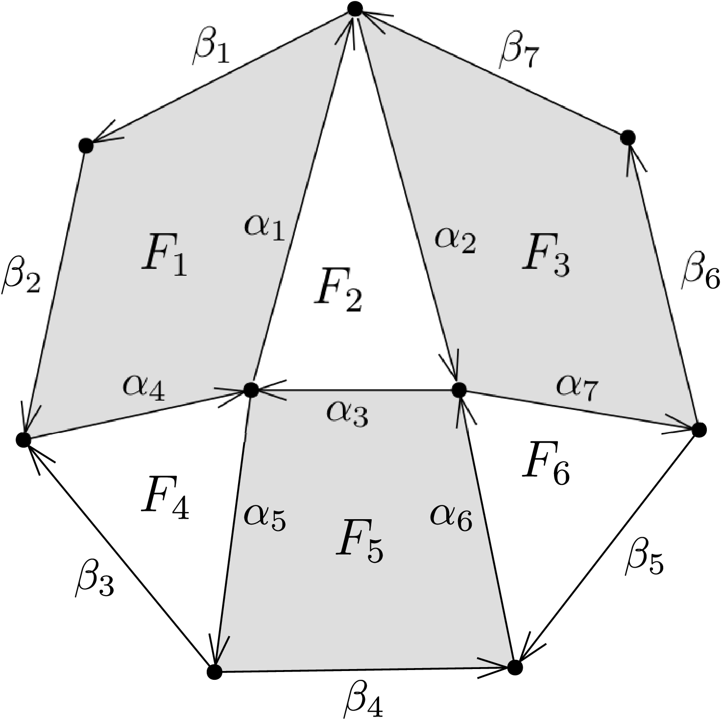
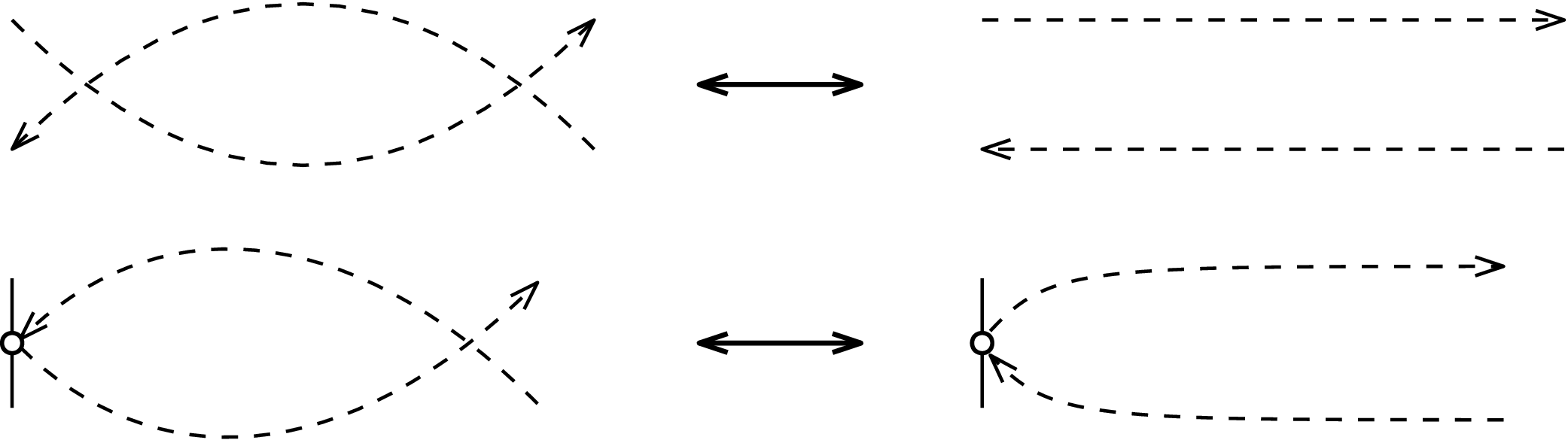
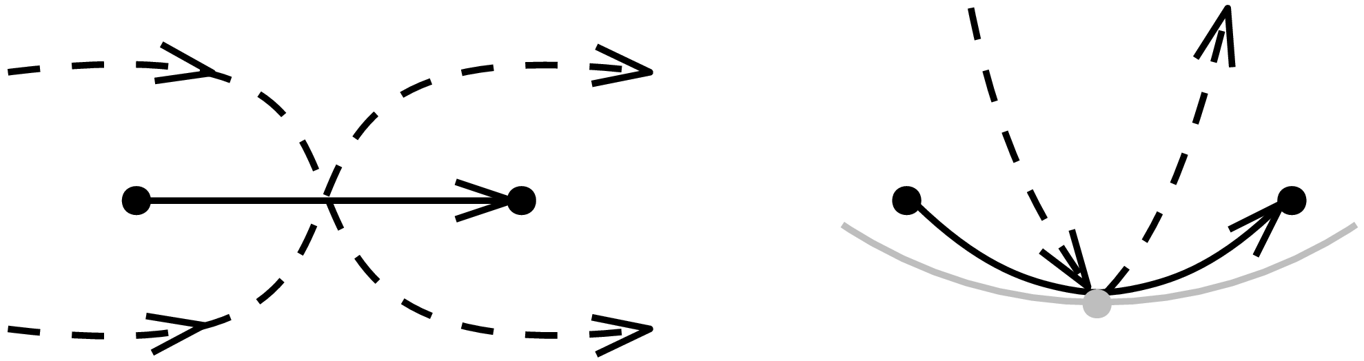
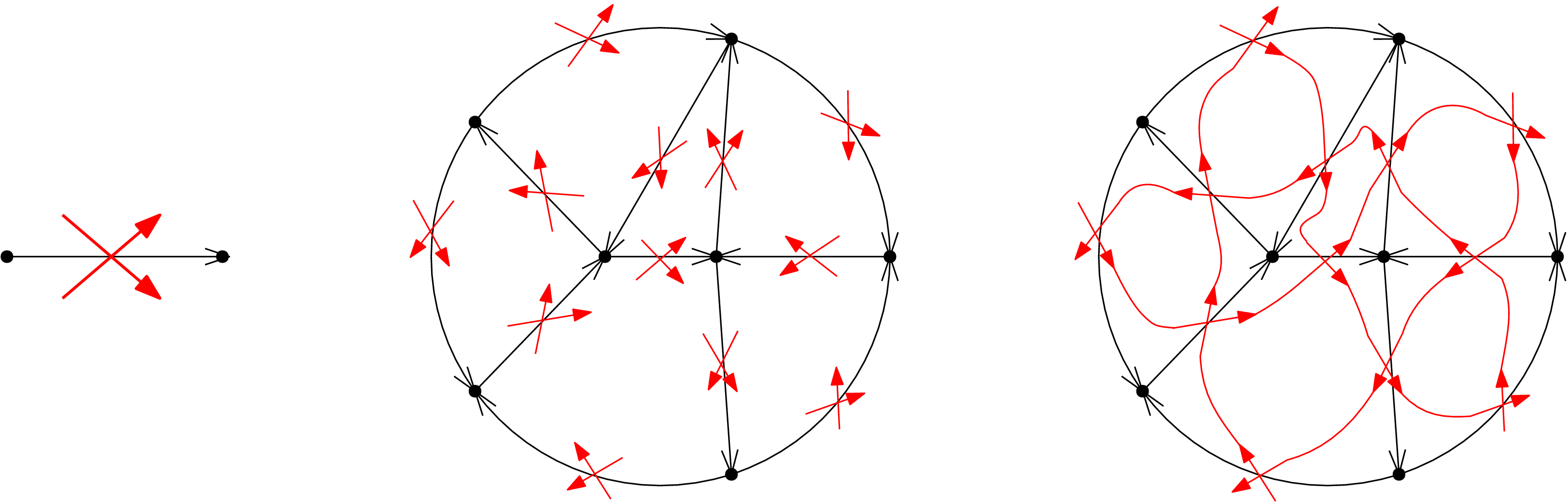
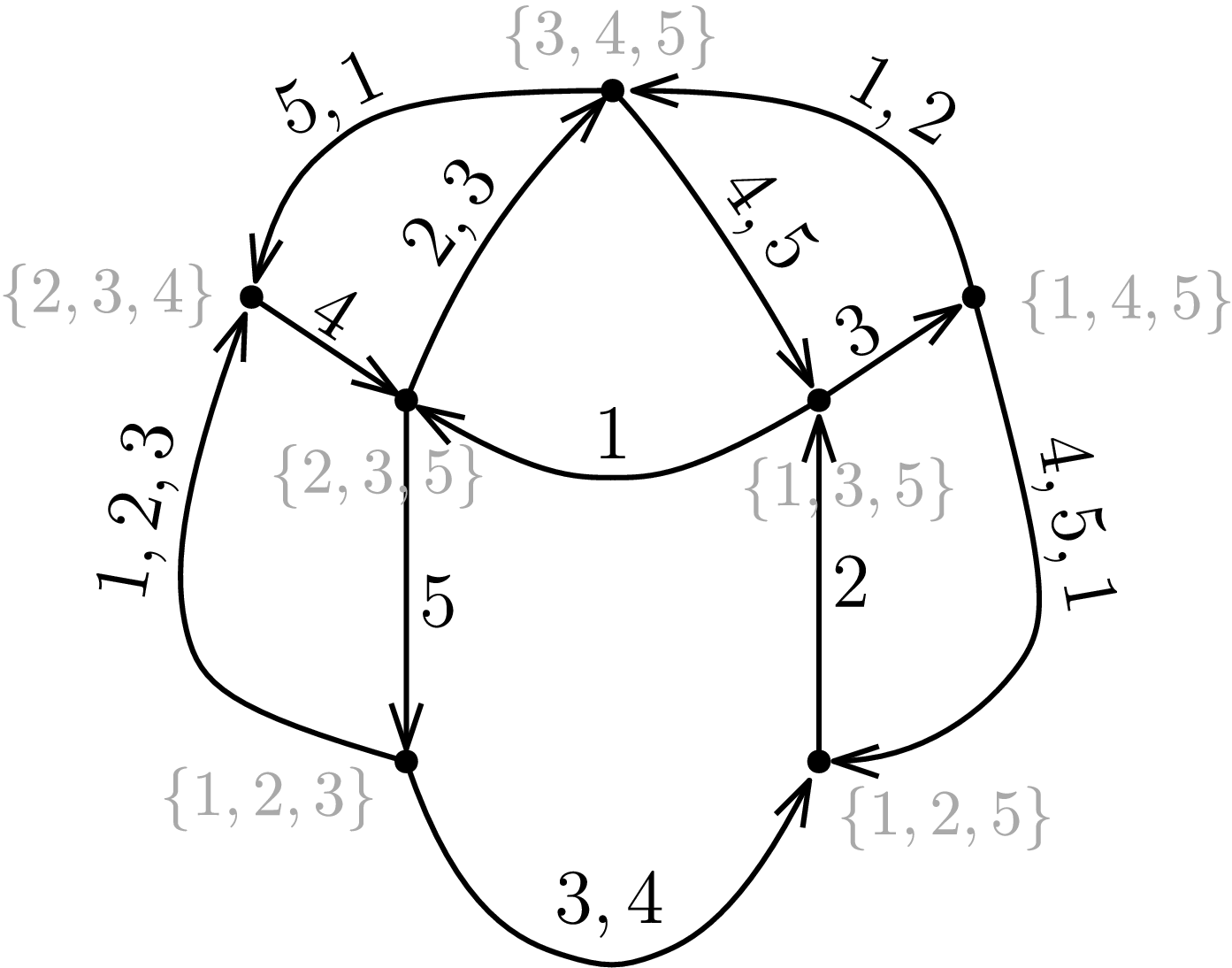
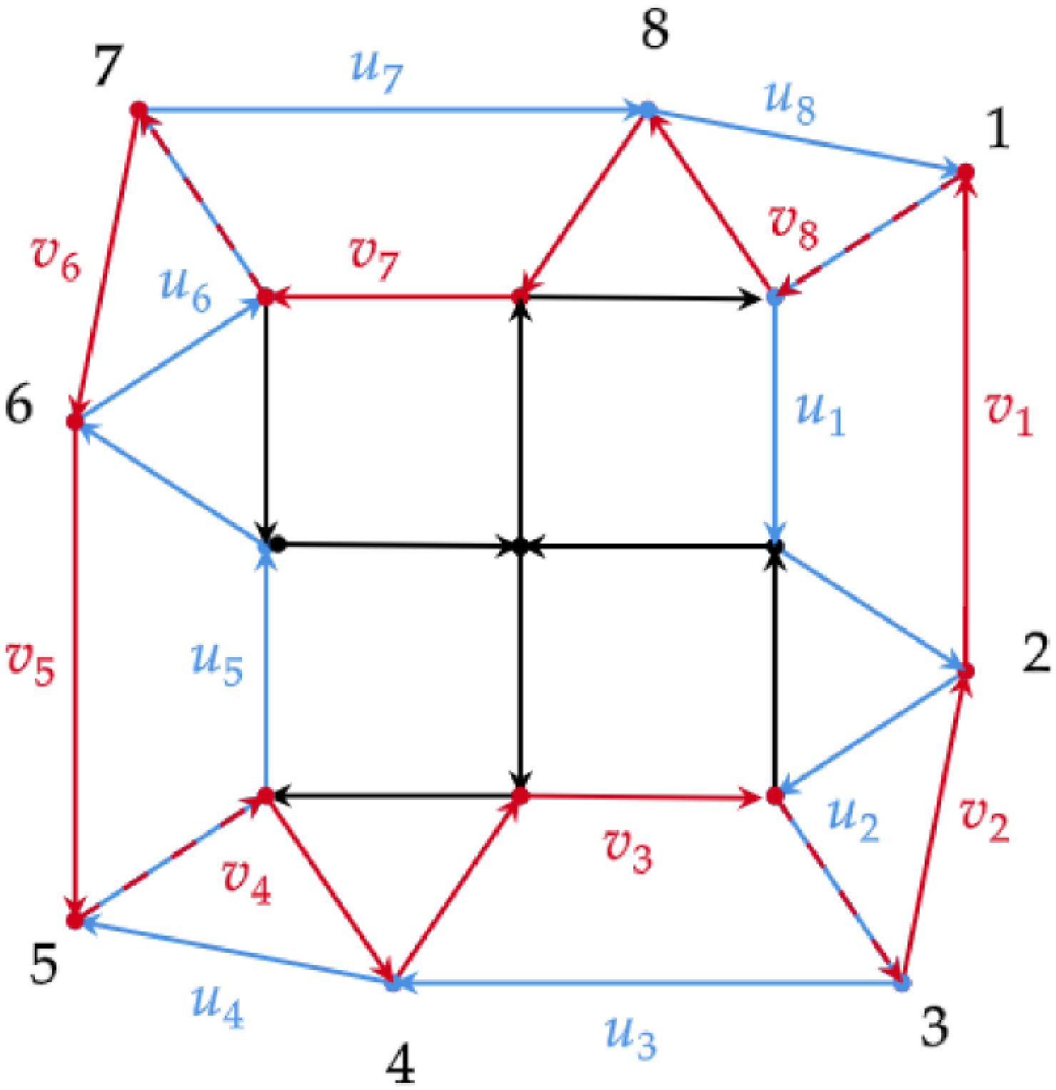


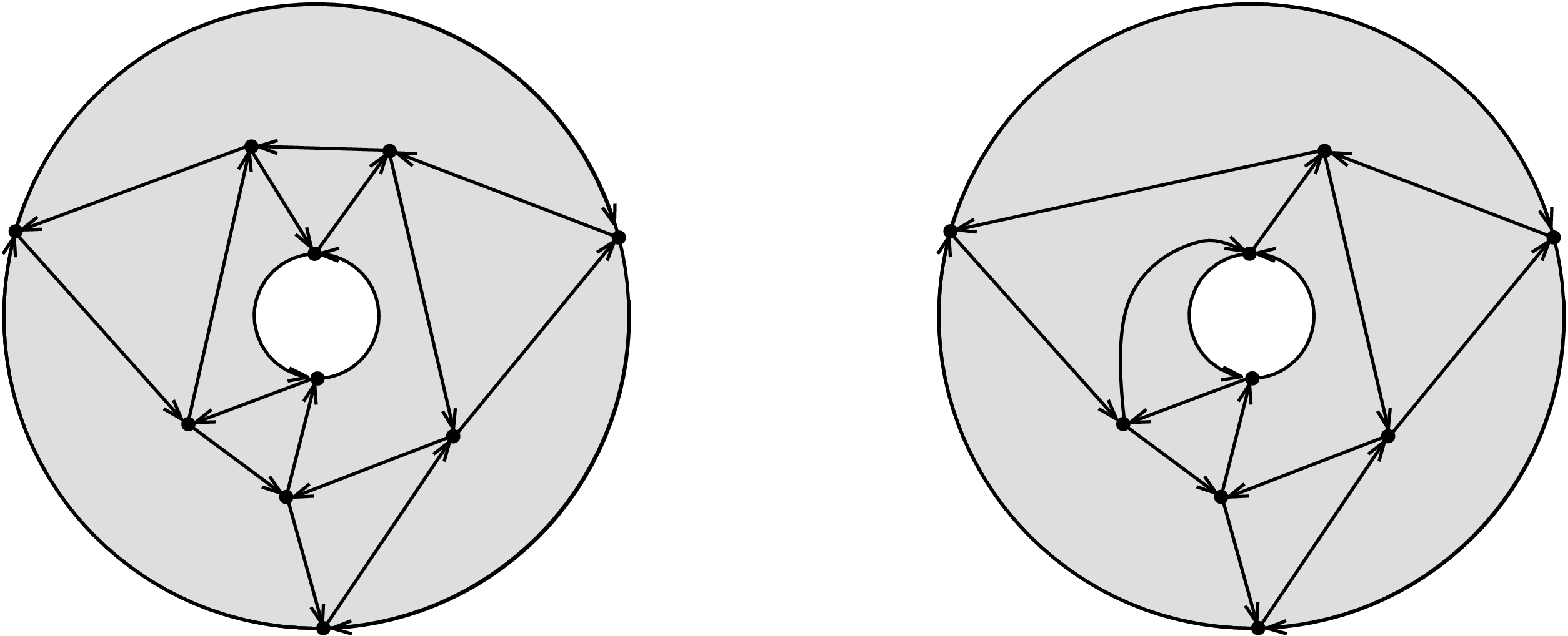
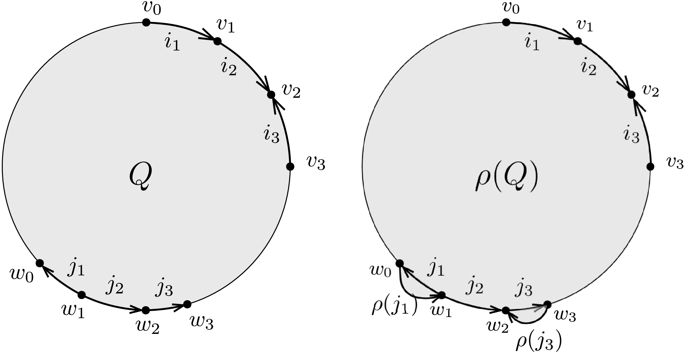


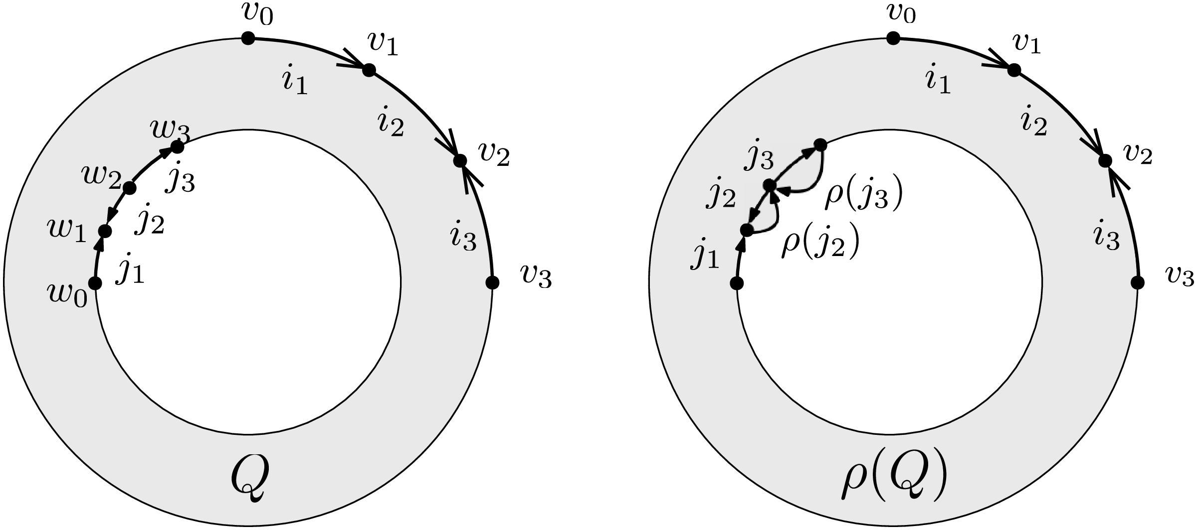


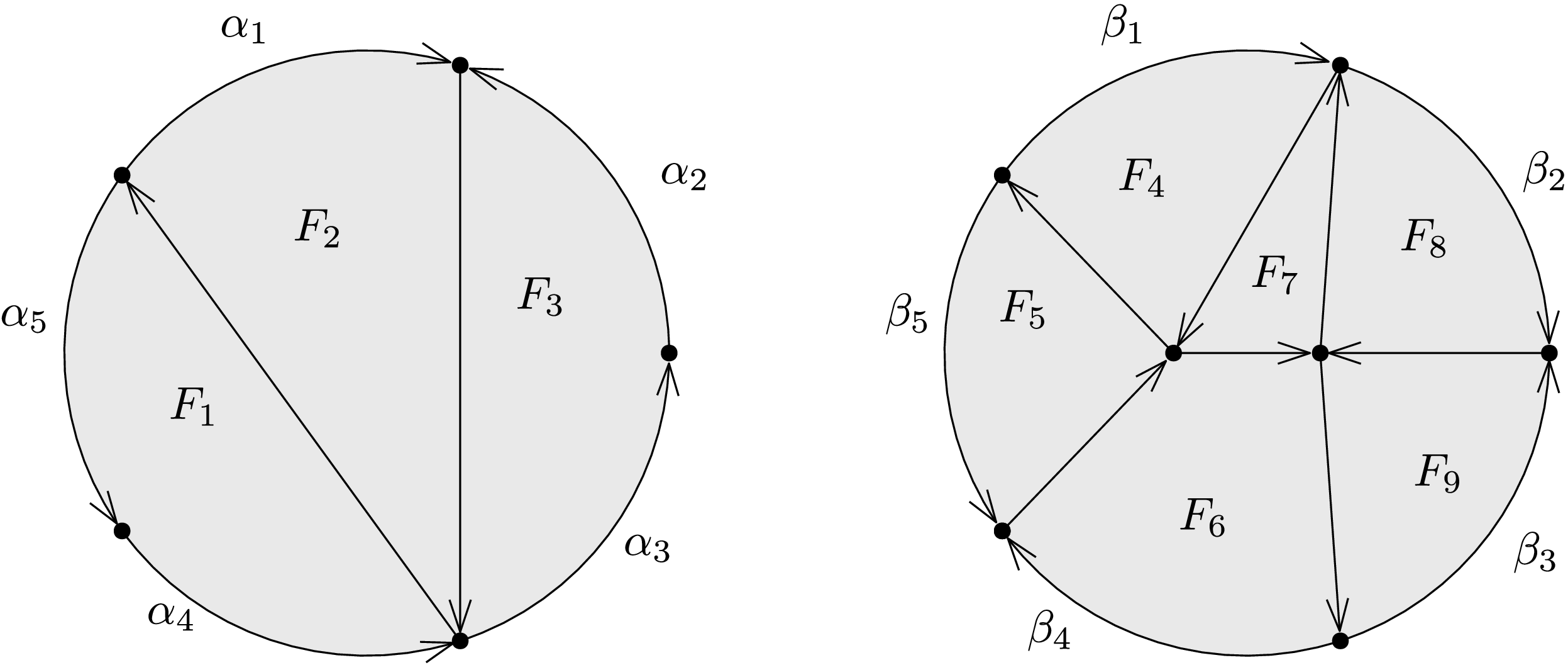

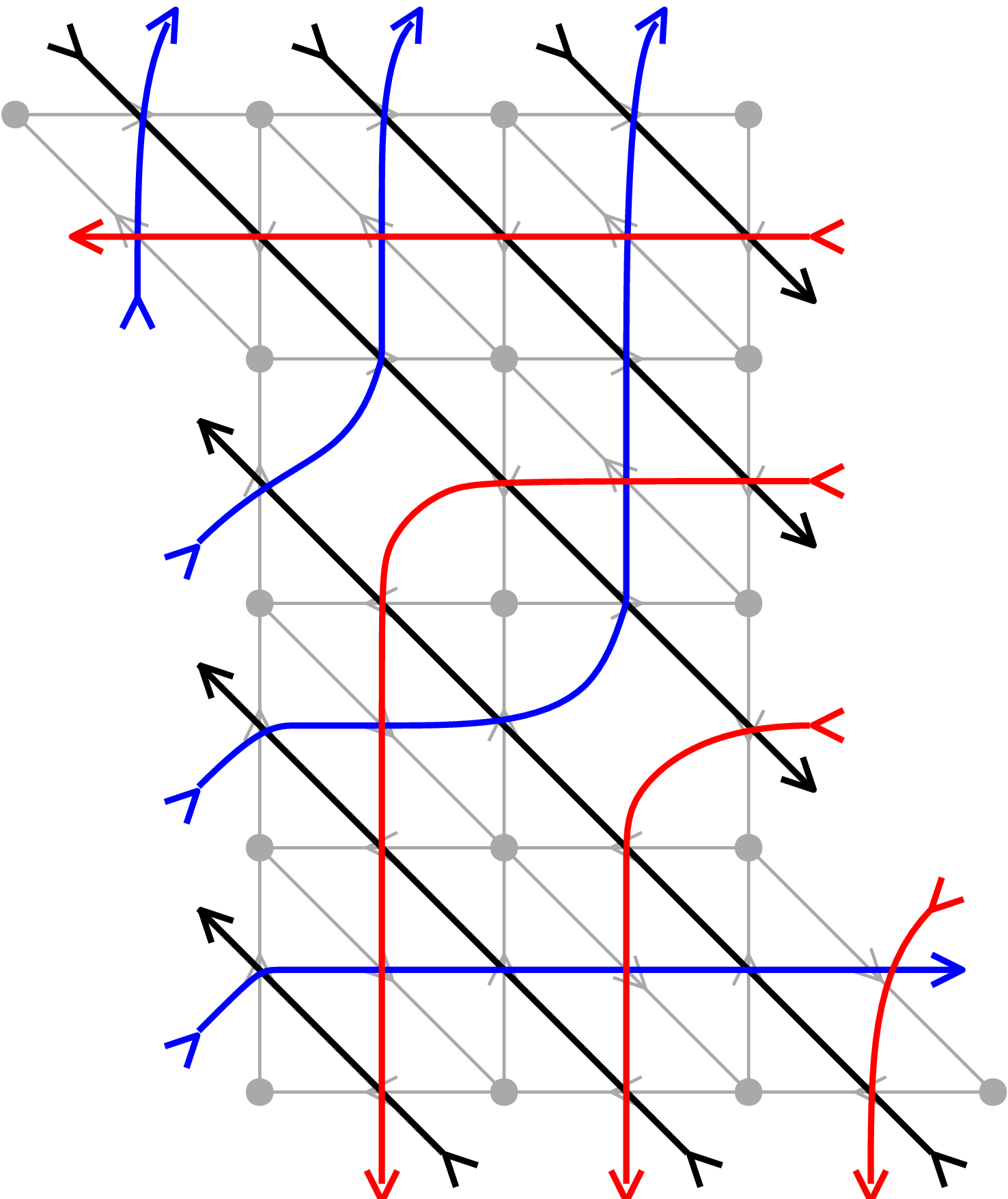

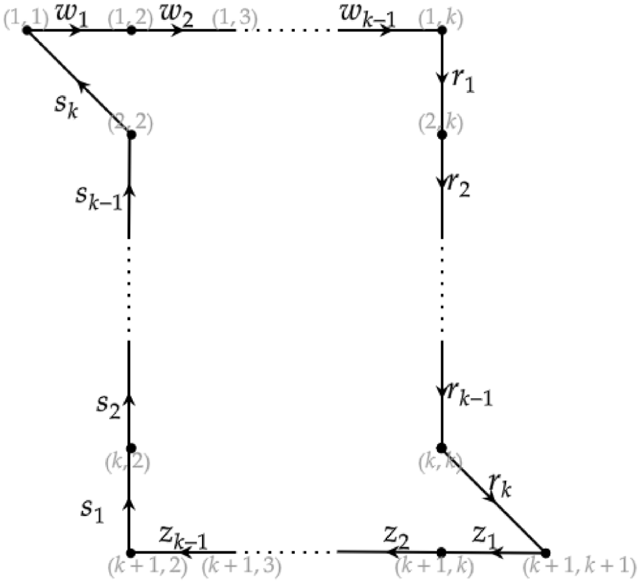

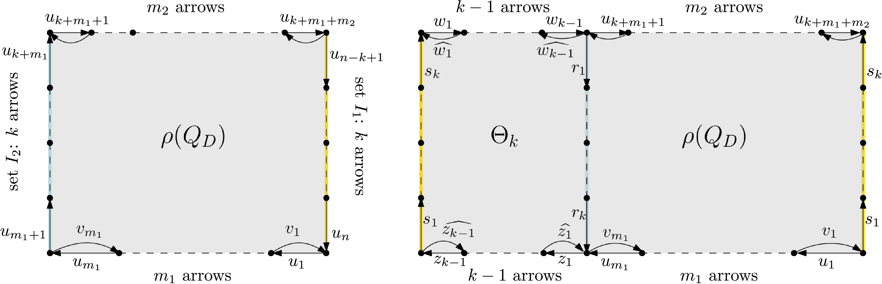


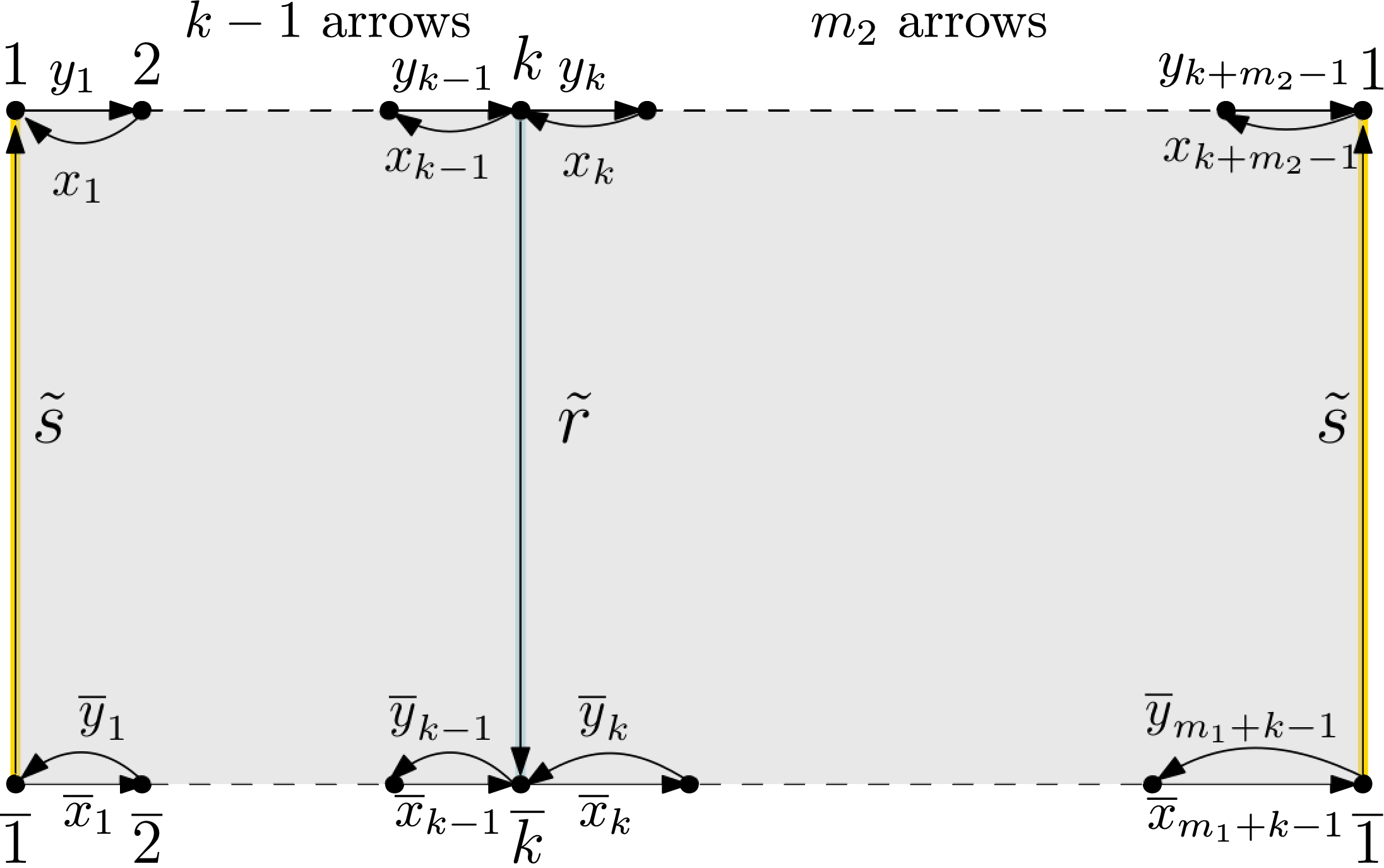

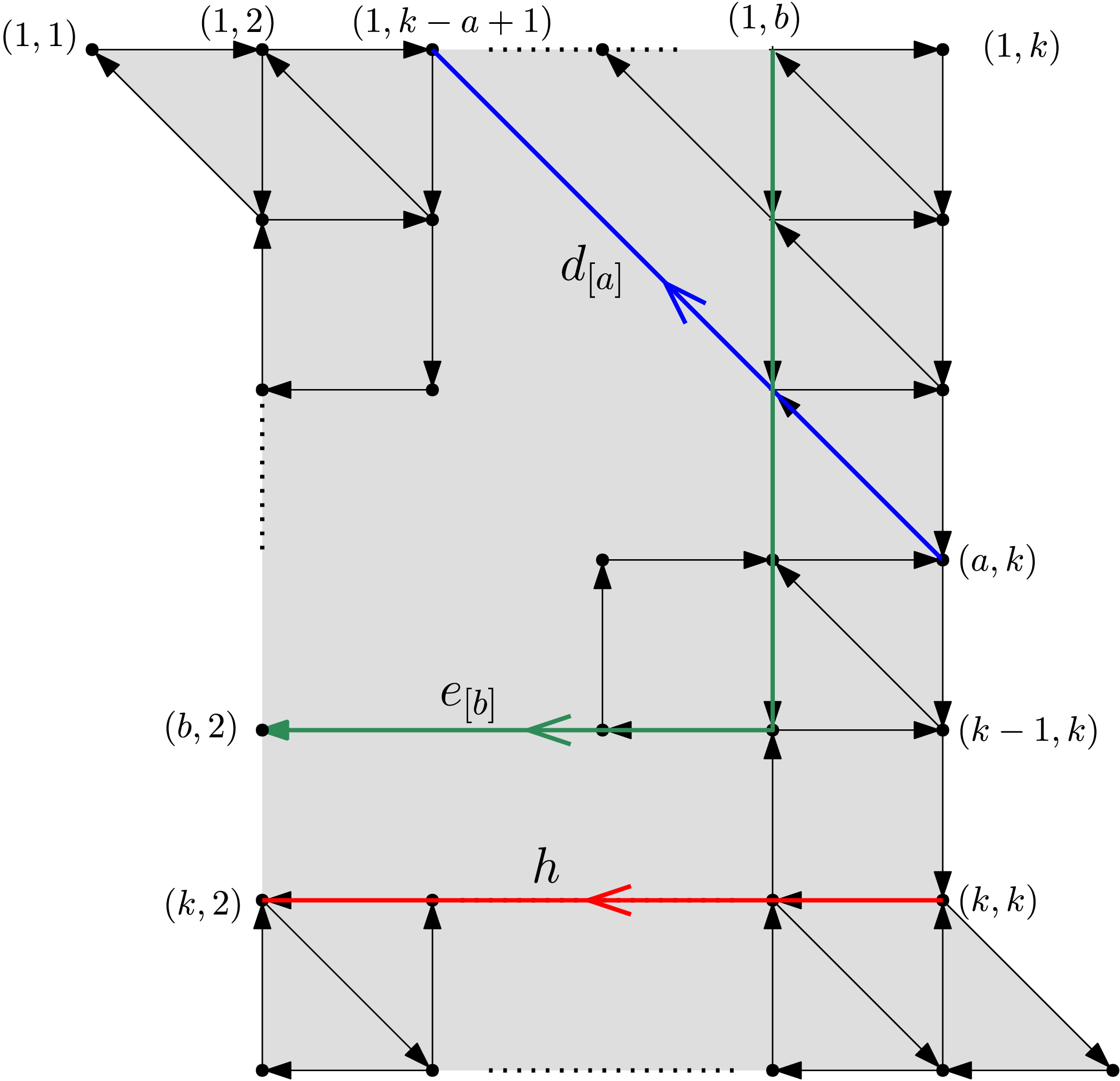


 Open access