


1 Introduction
1.1 The goal of this paper
The Robinson–Schensted–Knuth (RSK) correspondence is a fundamental bijection between matrices M with nonnegative integer entries, sometimes encoded by biwords $\pi $
, and pairs of semistandard tableaux
$\pi $
, and pairs of semistandard tableaux $(P,Q)$
[Reference Knuth54, Reference Robinson72, Reference Schensted76]. It represents one of the central tools in combinatorics, and its applications range from representation theory to probability. Along with a simple algorithmic description, the RSK correspondence possesses a surprising number of properties and symmetries. These have been central object of study throughout the 20th century, receiving contributions from a number of celebrated combinatorialists. A detailed account on the theory of RSK correspondence can be found in classical books as [Reference Fulton31, Reference Lothaire60, Reference Sagan74, Reference Stanley82].
$(P,Q)$
[Reference Knuth54, Reference Robinson72, Reference Schensted76]. It represents one of the central tools in combinatorics, and its applications range from representation theory to probability. Along with a simple algorithmic description, the RSK correspondence possesses a surprising number of properties and symmetries. These have been central object of study throughout the 20th century, receiving contributions from a number of celebrated combinatorialists. A detailed account on the theory of RSK correspondence can be found in classical books as [Reference Fulton31, Reference Lothaire60, Reference Sagan74, Reference Stanley82].
The RSK correspondence provides powerful tools to prove various identities involving symmetric functions. For instance the Cauchy identity for the Schur polynomials $s_{\lambda }$
, with
$s_{\lambda }$
, with $x=(x_1,\dots ,x_n)$
,
$x=(x_1,\dots ,x_n)$
, $y=(y_1,\dots ,y_n)$
,
$y=(y_1,\dots ,y_n)$
,
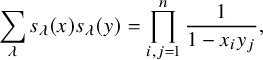 $$ \begin{align} \sum_{\lambda} s_{\lambda}(x) s_{\lambda}(y) = \prod_{i,j=1}^n \frac{1}{1-x_i y_j}, \end{align} $$
which can be proved in various ways, may also be seen as a consequence of the RSK correspondence. On the left-hand side the Schur polynomial appears as a result of the combinatorial formula $s_{\lambda }(x)=\sum _{T:{\mathrm sh} T=\lambda }x^T$
where the sum is over semistandard tableaux with shape
$s_{\lambda }(x)=\sum _{T:{\mathrm sh} T=\lambda }x^T$
where the sum is over semistandard tableaux with shape $\lambda $
, whereas each factor in the right-hand side is a geometric sum corresponding to each matrix element of an integral matrix M of size
$\lambda $
, whereas each factor in the right-hand side is a geometric sum corresponding to each matrix element of an integral matrix M of size $n \times n$
. An advantage of finding a bijective proof is that by leveraging symmetries it leads to a number of related identities; see for instance [Reference Stanley82].
$n \times n$
. An advantage of finding a bijective proof is that by leveraging symmetries it leads to a number of related identities; see for instance [Reference Stanley82].
A well-known property of the RSK is Schensted’s theorem [Reference Schensted76]. It says that, assuming
![]() , the length of the first row of tableaux
, the length of the first row of tableaux $P,Q$
equals the length of the longest increasing subsequence of the biword
$P,Q$
equals the length of the longest increasing subsequence of the biword $\pi $
. Noticeabl, this property became a crucial tool in the solution of the Ulam’s problem [Reference Baik, Deift and Johansson4, Reference Logan and Shepp59, Reference Vershik and Kerov87]. A generalization of Schensted’s theorem was found by Greene [Reference Greene36], who proved that the full shape of tableaux
$\pi $
. Noticeabl, this property became a crucial tool in the solution of the Ulam’s problem [Reference Baik, Deift and Johansson4, Reference Logan and Shepp59, Reference Vershik and Kerov87]. A generalization of Schensted’s theorem was found by Greene [Reference Greene36], who proved that the full shape of tableaux $P,Q$
can be identified by maximizing the disjoint increasing subsequences of
$P,Q$
can be identified by maximizing the disjoint increasing subsequences of $\pi $
or, alternatively, maximizing the passage times of disjoint directed paths through M. Greene’s characterization has found uses in the discovery of universal objects in probability theory such as the directed landscape [Reference Dauvergne, Ortmann and Virag24], which is a generalization of the Airy process [Reference Prähofer and Spohn70].
$\pi $
or, alternatively, maximizing the passage times of disjoint directed paths through M. Greene’s characterization has found uses in the discovery of universal objects in probability theory such as the directed landscape [Reference Dauvergne, Ortmann and Virag24], which is a generalization of the Airy process [Reference Prähofer and Spohn70].
In [Reference Sagan and Stanley73], Sagan and Stanley discovered a generalization of the RSK correspondence which relates pairs $(\overline {M};\nu )$
consisting of a matrix of sequences of nonnegative integers
$(\overline {M};\nu )$
consisting of a matrix of sequences of nonnegative integers $\overline {M}= (\overline {M}_{i,j}(k)\in \mathbb {N}_0 :i,j\in \{1,\dots ,n\},k\in \mathbb {N}_0)$
and a partition
$\overline {M}= (\overline {M}_{i,j}(k)\in \mathbb {N}_0 :i,j\in \{1,\dots ,n\},k\in \mathbb {N}_0)$
and a partition $\nu $
with pairs
$\nu $
with pairs $(P,Q)$
of semistandard tableaux of generic skew shape. Throughout, we will use the convention
$(P,Q)$
of semistandard tableaux of generic skew shape. Throughout, we will use the convention $\mathbb {N}=\{1,2,\dots \}$
and
$\mathbb {N}=\{1,2,\dots \}$
and $\mathbb {N}_0=\mathbb {N} \cup \{ 0 \}$
. In this paper, we will refer to this as Sagan–Stanley correspondence, and we will often use the shorthand
$\mathbb {N}_0=\mathbb {N} \cup \{ 0 \}$
. In this paper, we will refer to this as Sagan–Stanley correspondence, and we will often use the shorthand
![]() . Naturally, they also discussed an application of their correspondence to prove bijectively a Cauchy identity for skew Schur polynomials
. Naturally, they also discussed an application of their correspondence to prove bijectively a Cauchy identity for skew Schur polynomials $s_{\lambda /\rho }$
[Reference Macdonald62, Chapter I.5]. Fixing a parameter
$s_{\lambda /\rho }$
[Reference Macdonald62, Chapter I.5]. Fixing a parameter $|q|<1$
and variables
$|q|<1$
and variables $|x_i y_j|<1$
,
$|x_i y_j|<1$
, $i,j=1,\dots ,n$
, it reads
$i,j=1,\dots ,n$
, it reads
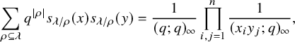 $$ \begin{align} \sum_{\rho \subseteq \lambda} q^{|\rho|} s_{\lambda/\rho}(x) s_{\lambda/\rho}(y) = \frac{1}{(q;q)_{\infty}} \prod_{i,j=1}^n \frac{1}{(x_i y_j; q)_{\infty}}, \end{align} $$
where $(z;q)_n =(1-z)(1-qz)\cdots (1-q^{n-1}z) ,n\in \mathbb {N}_0 \cup \{+\infty \}$
is the q-Pochhammer symbol.
$(z;q)_n =(1-z)(1-qz)\cdots (1-q^{n-1}z) ,n\in \mathbb {N}_0 \cup \{+\infty \}$
is the q-Pochhammer symbol.
Unlike for the classical RSK correspondence, a detailed description of properties of Sagan and Stanley’s algorithm has proven to be more challenging to obtain. Powerful tools such as Schützenberger’s theory of jeu de taquin [Reference Schützenberger78] do not admit straightforward ‘skew’ analogs and extensions of Greene invariants in a skew setting have also remained unexplored. For instance, if we assume
![]() , then a simple characterization of the last passage times of the matrix
, then a simple characterization of the last passage times of the matrix $\overline {M}$
, properly defined, in terms of tableaux
$\overline {M}$
, properly defined, in terms of tableaux $P,Q$
was, until the time of writing, not available. In this paper, we fill this void by introducing a dynamics on the set of pairs
$P,Q$
was, until the time of writing, not available. In this paper, we fill this void by introducing a dynamics on the set of pairs $(P,Q)$
and provide a generalization of Greene’s theorem in this skew setting, as a consequence of the theory we develop.
$(P,Q)$
and provide a generalization of Greene’s theorem in this skew setting, as a consequence of the theory we develop.
To people with experience in symmetric polynomials, the factorized expression in the right-hand side of identity (1.2) should look familiar. In fact, a closely resembling expression arises when considering the Cauchy identity for q-Whittaker polynomials $\mathscr {P}_{\mu }(x;q)$
[Reference Gerasimov, Lebedev and Oblezin34], that are Macdonald polynomials
$\mathscr {P}_{\mu }(x;q)$
[Reference Gerasimov, Lebedev and Oblezin34], that are Macdonald polynomials $\mathscr {P}_{\mu }(x;q,t)$
[Reference Macdonald62, Chapter VI] with parameter
$\mathscr {P}_{\mu }(x;q,t)$
[Reference Macdonald62, Chapter VI] with parameter $t=0$
. We have
$t=0$
. We have
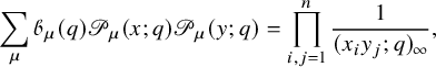
where
![]() is a normalization factor and its explicit definition can be found in equation (10.4) in the text. The Macdonald polynomials
is a normalization factor and its explicit definition can be found in equation (10.4) in the text. The Macdonald polynomials $\mathscr {P}_{\mu }(x;q,t)$
are widely considered as a central object in the theory of special functions and play prominent roles in various fields such as affine Hecke algebras [Reference Cherednik18], Hilbert schemes [Reference Haiman38], combinatorics [Reference Haglund, Haiman and Loehr37] and more recently in integrable probability [Reference Borodin and Corwin14] and integrable systems [Reference Cantini, de Gier and Wheeler17]. The particular case of the q-Whittaker polynomials has also attracted special attention in recent years because of their importance in integrable probability [Reference Borodin and Corwin14, Reference Imamura, Mucciconi and Sasamoto43, Reference Matveev and Petrov63, Reference O’Connell and Pei66, Reference Orr and Petrov68], representation theory [Reference Garsia and Procesi33, Reference Naito and Sagaki64, Reference Sanderson75, Reference Schilling and Tingley77], combinatorics [Reference Borodin and Wheeler15, Reference Cantini, de Gier and Wheeler17, Reference Garbali and Wheeler32] and a few other subjects. A proof of the Cauchy identity (1.3) is explained in [Reference Macdonald62]. Several different proofs have appeared in the literature in recent years, which are based on the Yang–Baxter equation [Reference Borodin and Wheeler15] or randomized variants of the RSK algorithm [Reference Matveev and Petrov63, Reference O’Connell and Pei66]. In [Reference Feigin, Khoroshkin and Makedonskyi26], representation-theoretic aspects of the Cauchy identity are investigated. However, to the best of the authors’ knowledge, none of the techniques available in the existing literature allow for a bijective proof of the Cauchy identity (1.3).
$\mathscr {P}_{\mu }(x;q,t)$
are widely considered as a central object in the theory of special functions and play prominent roles in various fields such as affine Hecke algebras [Reference Cherednik18], Hilbert schemes [Reference Haiman38], combinatorics [Reference Haglund, Haiman and Loehr37] and more recently in integrable probability [Reference Borodin and Corwin14] and integrable systems [Reference Cantini, de Gier and Wheeler17]. The particular case of the q-Whittaker polynomials has also attracted special attention in recent years because of their importance in integrable probability [Reference Borodin and Corwin14, Reference Imamura, Mucciconi and Sasamoto43, Reference Matveev and Petrov63, Reference O’Connell and Pei66, Reference Orr and Petrov68], representation theory [Reference Garsia and Procesi33, Reference Naito and Sagaki64, Reference Sanderson75, Reference Schilling and Tingley77], combinatorics [Reference Borodin and Wheeler15, Reference Cantini, de Gier and Wheeler17, Reference Garbali and Wheeler32] and a few other subjects. A proof of the Cauchy identity (1.3) is explained in [Reference Macdonald62]. Several different proofs have appeared in the literature in recent years, which are based on the Yang–Baxter equation [Reference Borodin and Wheeler15] or randomized variants of the RSK algorithm [Reference Matveev and Petrov63, Reference O’Connell and Pei66]. In [Reference Feigin, Khoroshkin and Makedonskyi26], representation-theoretic aspects of the Cauchy identity are investigated. However, to the best of the authors’ knowledge, none of the techniques available in the existing literature allow for a bijective proof of the Cauchy identity (1.3).
Nevertheless the striking similarity between partition functions (1.2), (1.3), along with the fact that all terms involved
![]() possess positive monomial expansions, suggest the possibility of relating the theories concerning the RSK correspondence to q-Whittaker polynomials. The goal of this paper is to develop a combinatorial theory extending the scope of the RSK correspondence and which allows the first bijective proof of the Cauchy identity (1.3). As a consequence our theory will produce a number of new identities involving q-Whittaker polynomials and we envision it playing important roles in a wide range of related fields in the future.
possess positive monomial expansions, suggest the possibility of relating the theories concerning the RSK correspondence to q-Whittaker polynomials. The goal of this paper is to develop a combinatorial theory extending the scope of the RSK correspondence and which allows the first bijective proof of the Cauchy identity (1.3). As a consequence our theory will produce a number of new identities involving q-Whittaker polynomials and we envision it playing important roles in a wide range of related fields in the future.
1.2 Skew RSK dynamics: examples and emerging questions
To achieve the goals outlined above, we first introduce a new deterministic time evolution on pairs of skew tableaux, which is defined by combining the skew RSK map introduced in [Reference Sagan and Stanley73] and a novel cyclic operation on tableaux. We call this the skew RSK dynamics, and in this subsection we will see through an example how it would bring a connection between skew tableaux and q-Whittaker polynomials. Looking at time evolution of skew tableaux for some examples, we observe certain properties of the dynamics and a few questions emerge. Indeed, results presented in this paper are obtained while proving these properties and answering these questions.
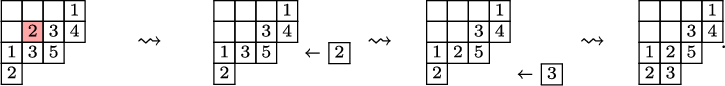
To define our dynamics, we first recall a basic operation on a tableau called the internal insertion, which was introduced in [Reference Sagan and Stanley73]. From a semistandard tableau of skew shape P, select a row r such that the leftmost cell $(c,r)$
at that row is a corner cell, that is, both
$(c,r)$
at that row is a corner cell, that is, both $(c-1,r)$
and
$(c-1,r)$
and $(c,r-1)$
are empty cells. Then,
$(c,r-1)$
are empty cells. Then, $\mathcal {R}_{[r]}(P)$
is the tableau obtained vacating the cell
$\mathcal {R}_{[r]}(P)$
is the tableau obtained vacating the cell $(c,r)$
of P and inserting, following the usual Schensted’s bumping algorithm, the value
$(c,r)$
of P and inserting, following the usual Schensted’s bumping algorithm, the value $P(c,r)$
at the row below. For a more precise description of this procedure, see Section 3.1 below. In the following example, calling P the tableau on the left-hand side, we show, step by step, the computation of
$P(c,r)$
at the row below. For a more precise description of this procedure, see Section 3.1 below. In the following example, calling P the tableau on the left-hand side, we show, step by step, the computation of $\mathcal {R}_{[2]}(P)$
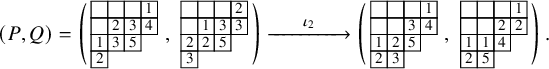
Using the notion of internal insertion, we define a new map, this time acting on pairs of skew tableaux $(P,Q)$
with the same shape. We call it
$(P,Q)$
with the same shape. We call it $\iota _2$
to emphasize its nontrivial action on the second tableaux Q; later in Section 1.3, we will also introduce
$\iota _2$
to emphasize its nontrivial action on the second tableaux Q; later in Section 1.3, we will also introduce $\iota _1$
. Entries of tableaux here are assumed to belong to the alphabet
$\iota _1$
. Entries of tableaux here are assumed to belong to the alphabet $\{1,\dots ,n\}$
for some fixed
$\{1,\dots ,n\}$
for some fixed $n\ge 1$
. Define
$n\ge 1$
. Define $\iota _2 : (P,Q) \mapsto ( P', Q' )$
, where
$\iota _2 : (P,Q) \mapsto ( P', Q' )$
, where $P' = \mathcal {R}_{[i_k]} \cdots \mathcal {R}_{[i_1]}(P)$
,
$P' = \mathcal {R}_{[i_k]} \cdots \mathcal {R}_{[i_1]}(P)$
, $i_1 \ge \dots \ge i_k$
are all row coordinates of
$i_1 \ge \dots \ge i_k$
are all row coordinates of $1$
-cells (i.e., cells with label 1) of Q, and
$1$
-cells (i.e., cells with label 1) of Q, and $Q'$
is obtained from Q vacating all
$Q'$
is obtained from Q vacating all $1$
-cells, decreasing by 1 the labels of all remaining cells and creating n-cells to make the shape of
$1$
-cells, decreasing by 1 the labels of all remaining cells and creating n-cells to make the shape of $P',Q'$
equal. The following example shows a realization of
$P',Q'$
equal. The following example shows a realization of $\iota _2(P,Q)$
, and we assume
$\iota _2(P,Q)$
, and we assume $n=5$
$n=5$
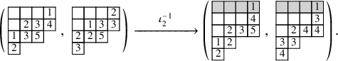
 $\iota _2$
is invertible, and the inverse
$\iota _2$
is invertible, and the inverse $\iota _2^{-1}$
is always well defined, provided we allow cells of tableaux to occupy also nonstrictly positive rows. To give a reference, while drawing tableaux we will color such cells in gray, so for instance we have
$\iota _2^{-1}$
is always well defined, provided we allow cells of tableaux to occupy also nonstrictly positive rows. To give a reference, while drawing tableaux we will color such cells in gray, so for instance we have
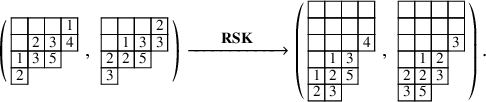
The operation $\iota _2$
, in particular the cycling operation on a Q tableau, is new in this paper and represents a dynamical rule preserving semistandard properties. Iterating n times the application of
$\iota _2$
, in particular the cycling operation on a Q tableau, is new in this paper and represents a dynamical rule preserving semistandard properties. Iterating n times the application of $\iota _2$
yields a known content preserving map, that in [Reference Sagan and Stanley73] was called ‘skew Knuth map’ and that we will call skew
$\iota _2$
yields a known content preserving map, that in [Reference Sagan and Stanley73] was called ‘skew Knuth map’ and that we will call skew $\mathbf {RSK}$
map,
$\mathbf {RSK}$
map,
For instance, we have
From (1.7), $\iota _2$
can be considered as a refinement of the skew
$\iota _2$
can be considered as a refinement of the skew $\mathbf {RSK}$
map. It will also play a crucial role when we discuss an affine bicrystal symmetry of the skew
$\mathbf {RSK}$
map. It will also play a crucial role when we discuss an affine bicrystal symmetry of the skew $\mathbf {RSK}$
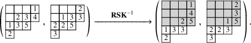
dynamics; see (1.25) below. The skew
$\mathbf {RSK}$
dynamics; see (1.25) below. The skew $\mathbf {RSK}$
map is invertible, and its inverse
$\mathbf {RSK}$
map is invertible, and its inverse $\mathbf {RSK}^{-1}$
comes from the application of n consecutive times of
$\mathbf {RSK}^{-1}$
comes from the application of n consecutive times of $\iota _2^{-1}$
. Continuing with our running example, we find
$\iota _2^{-1}$
. Continuing with our running example, we find
The skew $\mathbf {RSK}$
map is a map from a pair of skew tableaux to another. Iterating the map t times, one can define the time evolution of a pair of skew tableaux by
$\mathbf {RSK}$
map is a map from a pair of skew tableaux to another. Iterating the map t times, one can define the time evolution of a pair of skew tableaux by $(P_{t+1},Q_{t+1}) = \mathbf {RSK}^{t}(P,Q)$
, with the initial condition given by
$(P_{t+1},Q_{t+1}) = \mathbf {RSK}^{t}(P,Q)$
, with the initial condition given by $(P_1,Q_1)=(P,Q)$
. In this paper, we adopt the convention that the starting time of a dynamics is
$(P_1,Q_1)=(P,Q)$
. In this paper, we adopt the convention that the starting time of a dynamics is $t=1$
. Note that t can be an arbitrary integer, using
$t=1$
. Note that t can be an arbitrary integer, using $\mathbf {RSK}^{-1}$
for a negative t. We call this the skew
$\mathbf {RSK}^{-1}$
for a negative t. We call this the skew $\mathbf {RSK}$
dynamics, and it plays a central role in our theory.
$\mathbf {RSK}$
dynamics, and it plays a central role in our theory.
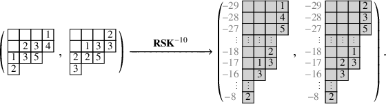
An interesting phenomenon occurs when we consider the large t limit. Tableaux $(P_t,Q_t)$
, from a certain t onward become ‘stable’, in the sense that the application of the skew
$(P_t,Q_t)$
, from a certain t onward become ‘stable’, in the sense that the application of the skew $\mathbf {RSK}$
map has the only effect of rigidly shifting columns downward. The amplitude of each shift is equal to the number of labeled cells at the column. Let us show this in our example taking, for instance,
$\mathbf {RSK}$
map has the only effect of rigidly shifting columns downward. The amplitude of each shift is equal to the number of labeled cells at the column. Let us show this in our example taking, for instance, $t=10$
. With some patience, one can compute
$t=10$
. With some patience, one can compute $\mathbf {RSK}^{10}(P,Q)$
as
$\mathbf {RSK}^{10}(P,Q)$
as
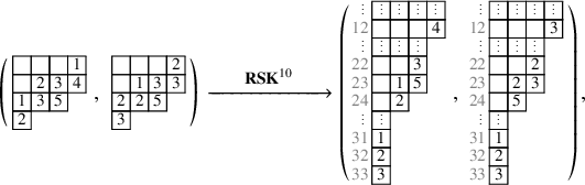
so that applying the skew $\mathbf {RSK}$
map one more time yields
$\mathbf {RSK}$
map one more time yields
In the previous two displays, the gray numbers to the left of the tableaux indicate the row coordinates of the cells to their right. We notice that, in equation (1.11), the skew $\mathbf {RSK}$
map had the only effect of shifting columns downward, as an instance of the stabilization phenomenon described just above. Notice again that in such stable states each column travels downward with ‘speed’ equal to the number of labeled cells it hosts. In the above example, the speeds are 3,2,2,1 for the first, second, third and fourth columns. Obviously, longer columns travel ‘faster’. This procedure defines an important object.
$\mathbf {RSK}$
map had the only effect of shifting columns downward, as an instance of the stabilization phenomenon described just above. Notice again that in such stable states each column travels downward with ‘speed’ equal to the number of labeled cells it hosts. In the above example, the speeds are 3,2,2,1 for the first, second, third and fourth columns. Obviously, longer columns travel ‘faster’. This procedure defines an important object.
Definition 1.1 (Asymptotic increments).
For a pair $(P,Q)$
of semistandard tableaux of the same skew shape, let
$(P,Q)$
of semistandard tableaux of the same skew shape, let $\lambda ^{t+1}/\rho ^{t+1}$
be the shape of the pair
$\lambda ^{t+1}/\rho ^{t+1}$
be the shape of the pair $\mathbf {RSK}^t(P,Q)$
. The asymptotic increment
$\mathbf {RSK}^t(P,Q)$
. The asymptotic increment $\mu (P,Q)$
is the partition defined by
$\mu (P,Q)$
is the partition defined by
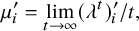 $$ \begin{align} \mu_i^{\prime} = \lim_{t \to \infty} (\lambda^t)_i^{\prime}/t, \end{align} $$
where $\lambda '$
means the transpose of
$\lambda '$
means the transpose of $\lambda $
, that is,
$\lambda $
, that is, $\lambda _i^{\prime }$
is the number of cells in the i-th column of
$\lambda _i^{\prime }$
is the number of cells in the i-th column of $\lambda $
.
$\lambda $
.
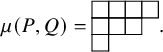
In other words, partition $\mu $
, defined by equation (1.12), is such that
$\mu $
, defined by equation (1.12), is such that $\mu _i^{\prime }$
is the speed of the i-th column of
$\mu _i^{\prime }$
is the speed of the i-th column of $(P_t,Q_t)$
, or the number of labeled cells eventually remaining in it, when t becomes large. It is an easy exercise to verify that limits (1.12) always exist and numbers
$(P_t,Q_t)$
, or the number of labeled cells eventually remaining in it, when t becomes large. It is an easy exercise to verify that limits (1.12) always exist and numbers $\mu _i^{\prime }$
define, in fact, an integer partition; see Proposition 4.15 below. In our example, we have
$\mu _i^{\prime }$
define, in fact, an integer partition; see Proposition 4.15 below. In our example, we have
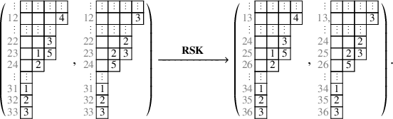
The same stabilization phenomenon happens when iterating the map $\mathbf {RSK}^{-1}$
, and we have, for instance,
$\mathbf {RSK}^{-1}$
, and we have, for instance,
A striking observation is that asymptotic increments of tableaux in the right-hand side of equations (1.10), (1.14) are equal, if we sort columns by length: In both cases, labeled cells eventually arrange themselves into four blocks which propagate with the same fixed speeds 3,2,2,1. This is not a coincidence. For any chosen pair of tableaux $P,Q$
, the ‘backward’ asymptotic increments one computes taking the limit
$P,Q$
, the ‘backward’ asymptotic increments one computes taking the limit $\mathbf {RSK}^{-t}(P,Q)$
for large t are always equal to
$\mathbf {RSK}^{-t}(P,Q)$
for large t are always equal to $\mu (P,Q)$
, after sorting columns by length. This strongly suggests that the asymptotic increments
$\mu (P,Q)$
, after sorting columns by length. This strongly suggests that the asymptotic increments $\mu $
record in fact conserved quantities of the skew
$\mu $
record in fact conserved quantities of the skew $\mathbf {RSK}$
dynamics throughout the time evolution, and the information of
$\mathbf {RSK}$
dynamics throughout the time evolution, and the information of $\mu $
may be contained already in
$\mu $
may be contained already in $(P,Q)$
. This leads us to the first major question.
$(P,Q)$
. This leads us to the first major question.
Question 1. Can we characterize the asymptotic increment $\mu $
in terms of the initial data
$\mu $
in terms of the initial data $(P,Q)$
?
$(P,Q)$
?
We will answer this question in Proposition 1.2 and in Proposition 6.6 in the text. Moreover, the equivalence between backward and forward asymptotic increment will be addressed by result in Proposition 9.1.
The existence of conservation laws suggests that the skew $\mathbf {RSK}$
dynamics admits a description as an integrable system. In fact, the skew
$\mathbf {RSK}$
dynamics admits a description as an integrable system. In fact, the skew $\mathbf {RSK}$
dynamics show a clear resemblance to the multispecies Box–Ball system (BBS), which is a well-known discrete classical integrable system [Reference Hatayama, Hikami, Inoue, Kuniba, Takagi and Tokihiro40, Reference Takahashi83–Reference Tokihiro, Nagai and Satsuma85] (see [Reference Inoue, Kuniba and Takagi46] for a review). We find such perspective particularly insightful. In this language, columns of tableaux become solitons. When
$\mathbf {RSK}$
dynamics show a clear resemblance to the multispecies Box–Ball system (BBS), which is a well-known discrete classical integrable system [Reference Hatayama, Hikami, Inoue, Kuniba, Takagi and Tokihiro40, Reference Takahashi83–Reference Tokihiro, Nagai and Satsuma85] (see [Reference Inoue, Kuniba and Takagi46] for a review). We find such perspective particularly insightful. In this language, columns of tableaux become solitons. When $t \ll 0$
, they are well separated and travel independently with their own speeds. At some point, they interact with each other through collisions that momentarily mess up their structure. Once mutual interactions end, they recover their original shape and again propagate with the same speed as before. A profound result in the theory of classical integrable systems is that the whole time evolution of such a system is fully determined by the knowledge of the scattering rules. These consist in the precise description of exchange of degrees of freedom (i.e., how content of columns changes between backward and forward aysmptotic states) and of the phase shift, which in our context are the shifts in asymptotic positions of solitons as compared to the ones anticipated from initial positions and speeds assuming no interaction occurs.
$t \ll 0$
, they are well separated and travel independently with their own speeds. At some point, they interact with each other through collisions that momentarily mess up their structure. Once mutual interactions end, they recover their original shape and again propagate with the same speed as before. A profound result in the theory of classical integrable systems is that the whole time evolution of such a system is fully determined by the knowledge of the scattering rules. These consist in the precise description of exchange of degrees of freedom (i.e., how content of columns changes between backward and forward aysmptotic states) and of the phase shift, which in our context are the shifts in asymptotic positions of solitons as compared to the ones anticipated from initial positions and speeds assuming no interaction occurs.
A natural question here is the following.
Question 2. Can we describe the scattering rules of the skew $\mathbf {RSK}$
dynamics?
$\mathbf {RSK}$
dynamics?
The answer to such questions from the point of view of solition theory will be provided in Section 9.
The asymptotic increment $\mu $
was defined to be a partition such that
$\mu $
was defined to be a partition such that $\mu _i^{\prime }$
is the number of labeled cells of the i-th column in
$\mu _i^{\prime }$
is the number of labeled cells of the i-th column in $P_t,Q_t$
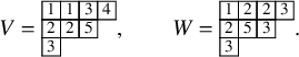
for large t. Recording labels eventually remaining on each column of
$P_t,Q_t$
for large t. Recording labels eventually remaining on each column of $P_t,Q_t$
, we can construct two tableaux
$P_t,Q_t$
, we can construct two tableaux $V,W$
, each of which consists of columns of increasing numbers. We will refer to these as vertically strict tableaux, and they differ from semistandard tableaux in that there is no condition on rows.Footnote
1
This defines a projection map
$V,W$
, each of which consists of columns of increasing numbers. We will refer to these as vertically strict tableaux, and they differ from semistandard tableaux in that there is no condition on rows.Footnote
1
This defines a projection map $\Phi $
from a pair of skew tableaux
$\Phi $
from a pair of skew tableaux $(P,Q)$
to a pair of vertically strict tableaux
$(P,Q)$
to a pair of vertically strict tableaux $(V, W)$
. In the example, we are considering in this section, from equation (1.10) we can write
$(V, W)$
. In the example, we are considering in this section, from equation (1.10) we can write $\Phi (P,Q) = ( V,W )$
, with
$\Phi (P,Q) = ( V,W )$
, with
Vertically strict tableaux, though much less studied compared to semistandard tableaux, play an important role in our theory because their generating function, with suitable weights, is known to produce the q-Whittaker polynomial [Reference Nakayashiki and Yamada65, Reference Sanderson75, Reference Schilling and Tingley77]; see equation (1.32) below. This opens up a possibility to understand Cauchy type summation identities involving q-Whittaker polynomials in a bijective fashion. In order to do so, we need to account for the information we lose while projecting, through $\Phi $
, a pair of tableaux
$\Phi $
, a pair of tableaux $(P,Q)$
to the corresponding vertically strict tableaux
$(P,Q)$
to the corresponding vertically strict tableaux $(V,W)$
. Then we arrive at the following question.
$(V,W)$
. Then we arrive at the following question.
Question 3. Can we refine projection $\Phi $
into a bijection?
$\Phi $
into a bijection?
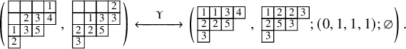
The answer to this third question represents a fundamental problem we solve in this paper. The refined map $\Upsilon $
, which will be described in Section 1.3 and Section 8, yields a bijection between pairs
$\Upsilon $
, which will be described in Section 1.3 and Section 8, yields a bijection between pairs $(P,Q)$
of skew tableaux and pairs of vertically strict tableaux
$(P,Q)$
of skew tableaux and pairs of vertically strict tableaux $(V,W)$
plus some ‘additional data’ characterizing, for instance, the shape of
$(V,W)$
plus some ‘additional data’ characterizing, for instance, the shape of $\mathbf {RSK}^t(P,Q)$
for large t.
$\mathbf {RSK}^t(P,Q)$
for large t.
1.3 Results, ideas and tools, and applications
There are two main results in this paper: the characterization of asymptotic increment $\mu (P,Q)$
as Greene invariants and the construction of the bijection
$\mu (P,Q)$
as Greene invariants and the construction of the bijection $\Upsilon $
. The first result answers Question 1. The second one, while being a direct answer to Question 3, also resolves Question 2. An application of bijection
$\Upsilon $
. The first result answers Question 1. The second one, while being a direct answer to Question 3, also resolves Question 2. An application of bijection $\Upsilon $
, leads to summation identities involving q-Whittaker polynomials. In the following paragraphs, we explain these results together with main ideas and tools to obtain them.
$\Upsilon $
, leads to summation identities involving q-Whittaker polynomials. In the following paragraphs, we explain these results together with main ideas and tools to obtain them.
1.3.1 Generalized Greene invariants
In the previous subsection, we hinted how the asymptotic increment $\mu (P,Q)$
records certain conserved quantities of the skew
$\mu (P,Q)$
records certain conserved quantities of the skew $\mathbf {RSK}$
dynamics, result that we will prove in Proposition 6.6. In order to explain these conservation laws, we find that algorithmic description of the skew
$\mathbf {RSK}$
dynamics, result that we will prove in Proposition 6.6. In order to explain these conservation laws, we find that algorithmic description of the skew $\mathbf {RSK}$
map given in terms of Schensted’s bumping algorithm is not particularly insightful. Instead, we employ a geometrical visualization of the RSK correspondence through Viennot’s shadow line construction [Reference Viennot88]. An analogous geometric realization can be devised for the Sagan–Stanley correspondence, where Viennot’s shadow lines are ‘drawn’ in a lattice with periodic geometry that we call a twisted cylinder.
$\mathbf {RSK}$
map given in terms of Schensted’s bumping algorithm is not particularly insightful. Instead, we employ a geometrical visualization of the RSK correspondence through Viennot’s shadow line construction [Reference Viennot88]. An analogous geometric realization can be devised for the Sagan–Stanley correspondence, where Viennot’s shadow lines are ‘drawn’ in a lattice with periodic geometry that we call a twisted cylinder.
For a natural number n, the twisted cylinder $\mathscr {C}_n$
can be represented as an infinite vertical strip
$\mathscr {C}_n$
can be represented as an infinite vertical strip $\{1,\dots ,n\} \times \mathbb {Z}$
, where we impose faces
$\{1,\dots ,n\} \times \mathbb {Z}$
, where we impose faces $(n,i)$
and
$(n,i)$
and $(1,i+n)$
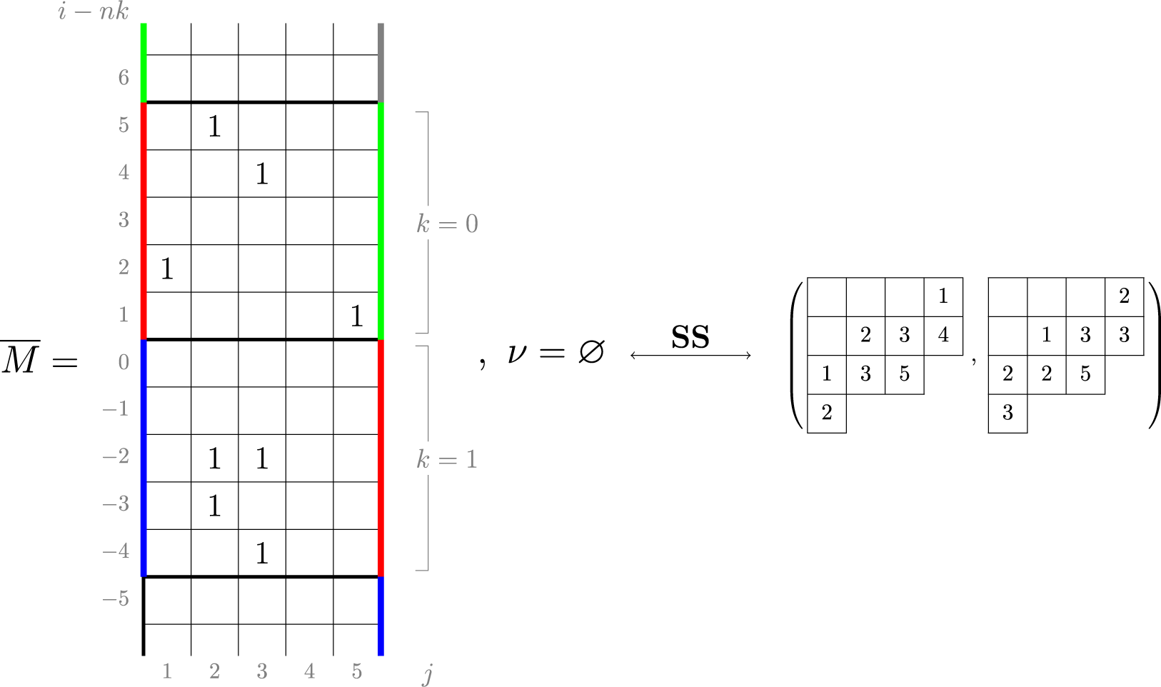
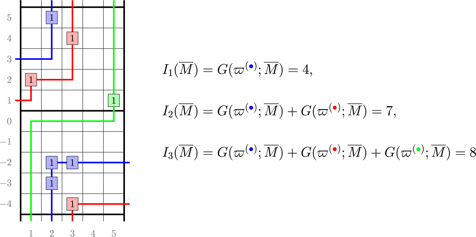
to be adjacent for all i; see Figure 1. For a more precise definition, see Section 4.3. A matrix of nonnegative integer sequences
$(1,i+n)$
to be adjacent for all i; see Figure 1. For a more precise definition, see Section 4.3. A matrix of nonnegative integer sequences $\overline {M}=(\overline {M}_{i,j}(k):i,j\in \{1,\dots ,n\}, k\in \mathbb {N}_0)$
can be represented as a map
$\overline {M}=(\overline {M}_{i,j}(k):i,j\in \{1,\dots ,n\}, k\in \mathbb {N}_0)$
can be represented as a map $\overline {M}:\mathscr {C}_n \to \mathbb {N}_0$
by settingFootnote
2
$\overline {M}:\mathscr {C}_n \to \mathbb {N}_0$
by settingFootnote
2
 $$ \begin{align} \overline{M}(j,i-kn) = \overline{M}_{i,j}(k), \qquad \text{for all} \qquad i,j\in\{1,\dots ,n\}, k\in \mathbb{N}_0, \end{align} $$
with a slight abuse of notation. In this new representation the Sagan–Stanley correspondence, described in Section 4.3 below, gives a bijection between compactly supported fillings $\overline {M}$
of
$\overline {M}$
of $\mathscr {C}_n$
and partitions
$\mathscr {C}_n$
and partitions $\nu $
to pairs of tableaux. As an example, such correspondence applied to the pair
$\nu $
to pairs of tableaux. As an example, such correspondence applied to the pair $(P,Q)$
used in Section 1.2 above appears in Figure 1 where, for the sake of cleaner notation we left cells
$(P,Q)$
used in Section 1.2 above appears in Figure 1 where, for the sake of cleaner notation we left cells $(j,i)$
of
$(j,i)$
of $\mathscr {C}_n$
empty whenever
$\mathscr {C}_n$
empty whenever $\overline {M}(j,i)=0$
. In the same figure, the entries of
$\overline {M}(j,i)=0$
. In the same figure, the entries of $\overline {M}$
are taken, for simplicity, to be all 0 or 1, although in general we have
$\overline {M}$
are taken, for simplicity, to be all 0 or 1, although in general we have $\overline {M}_{i,j}(k)\in \mathbb {N}_0$
. In case all entries
$\overline {M}_{i,j}(k)\in \mathbb {N}_0$
. In case all entries $\overline {M}_{i,j}(k)=0$
for
$\overline {M}_{i,j}(k)=0$
for $k \neq 0$
such representation reduces to the Matrix–Ball construction by Fulton [Reference Fulton31] and the Sagan–Stanley correspondence becomes the usual RSK.
$k \neq 0$
such representation reduces to the Matrix–Ball construction by Fulton [Reference Fulton31] and the Sagan–Stanley correspondence becomes the usual RSK.
A realization of the Sagan–Stanley correspondence
![]() . The matrix
. The matrix $\overline {M}$
is represented as a filling of the twisted cylinder
$\overline {M}$
is represented as a filling of the twisted cylinder $\mathscr {C}_5$
. Solid colored lines are identified by periodicity.
$\mathscr {C}_5$
. Solid colored lines are identified by periodicity.
An up-right path $\varpi $
on the twisted cylinder is a sequence
$\varpi $
on the twisted cylinder is a sequence $(\varpi _{\ell }: \ell \in \mathbb {Z}) \subset \mathscr {C}_n$
such that
$(\varpi _{\ell }: \ell \in \mathbb {Z}) \subset \mathscr {C}_n$
such that
 $$ \begin{align} \varpi_{\ell+1} \sim_n \varpi_{\ell} + \mathbf{e}_1, \qquad \text{or} \qquad \varpi_{\ell+1} \sim_n \varpi_{\ell} + \mathbf{e}_2, \qquad \text{for all } \ell \in \mathbb{Z}, \end{align} $$
where $\sim _n$
means the equivalence relation such that
$\sim _n$
means the equivalence relation such that $\mathscr {C}_n = \mathbb {Z}^2/\sim _n$
; see Proposition 4.2 in the text. Examples of up-right paths are colored trajectories in Figure 2. Notice that the up-right condition, along with the geometry of
$\mathscr {C}_n = \mathbb {Z}^2/\sim _n$
; see Proposition 4.2 in the text. Examples of up-right paths are colored trajectories in Figure 2. Notice that the up-right condition, along with the geometry of $\mathscr {C}_n$
implies that
$\mathscr {C}_n$
implies that $\varpi $
is not self-intersecting. Define the passage time of an up-right path
$\varpi $
is not self-intersecting. Define the passage time of an up-right path $\varpi $
as
$\varpi $
as
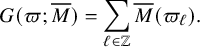 $$ \begin{align} G(\varpi;\overline{M}) = \sum_{\ell \in \mathbb{Z}} \overline{M}(\varpi_{\ell}). \end{align} $$
Objects as passage times are standard in the context of the RSK correspondence [Reference Greene36], although in classical setting endpoints of paths are usually fixed. In our case, up-right paths are always infinite and have no endpoints. Define the last passage time of k disjoint paths
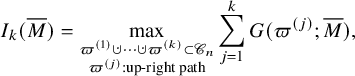
where
![]() denotes the disjoint union. For the map
denotes the disjoint union. For the map $\overline {M}$
given in Figure 1, all last passage times can be computed explicitly, as done in Figure 2. It is in general not true that the maximizer is unique or that in order to maximize the passage time for
$\overline {M}$
given in Figure 1, all last passage times can be computed explicitly, as done in Figure 2. It is in general not true that the maximizer is unique or that in order to maximize the passage time for $k+1$
paths it suffices to add an up-right path to a maximizing list of k paths.
$k+1$
paths it suffices to add an up-right path to a maximizing list of k paths.
Up-right paths
![]() maximize the passage times.
maximize the passage times.
The first original result we present relates last passage times of a matrix $\overline {M}$
with the asymptotic increment
$\overline {M}$
with the asymptotic increment $\mu $
of pair of tableaux
$\mu $
of pair of tableaux $(P,Q)$
corresponding to
$(P,Q)$
corresponding to $\overline {M}$
under Sagan–Stanley correspondence. We think of this as a generalization of Greene’s theorem [Reference Greene36].
$\overline {M}$
under Sagan–Stanley correspondence. We think of this as a generalization of Greene’s theorem [Reference Greene36].
Theorem 1.2 (Corollary of Proposition 6.6 in the text).
Consider
![]() , and let
, and let $\mu =\mu (P,Q)$
be the asymptotic increment of
$\mu =\mu (P,Q)$
be the asymptotic increment of $(P,Q)$
under the skew
$(P,Q)$
under the skew $\mathbf {RSK}$
dynamics. Then we have
$\mathbf {RSK}$
dynamics. Then we have
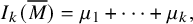 $$ \begin{align} I_k(\overline{M}) = \mu_1 + \cdots + \mu_k, \end{align} $$
for all $k=1,2,\dots $
.
$k=1,2,\dots $
.
The reader can check the validity of Proposition 1.2 comparing $\mu $
of equation (1.13) and last passage times in Figure 2. Motivated by equation (1.20), in the text we will often refer to the partition
$\mu $
of equation (1.13) and last passage times in Figure 2. Motivated by equation (1.20), in the text we will often refer to the partition $\mu (P,Q)$
as Greene invariant. We will see in Section 6 that the statistic
$\mu (P,Q)$
as Greene invariant. We will see in Section 6 that the statistic $\mu $
is indeed invariant with respect to a number of operations on
$\mu $
is indeed invariant with respect to a number of operations on $(P,Q)$
including (generalized) Knuth relations, Kashiwara operators and skew
$(P,Q)$
including (generalized) Knuth relations, Kashiwara operators and skew $\mathbf {RSK}$
map. In Proposition 6.6, an additional characterization of
$\mathbf {RSK}$
map. In Proposition 6.6, an additional characterization of $\mu (P,Q)$
is given, in terms of maximizing closed loops on the twisted cylinder. This represents an additional generalization of the Greene’s theorem [Reference Sagan74, Chapter 3].
$\mu (P,Q)$
is given, in terms of maximizing closed loops on the twisted cylinder. This represents an additional generalization of the Greene’s theorem [Reference Sagan74, Chapter 3].
The following result is an extension in skew setting of the classical Schensted’s theorem [Reference Schensted76]. It is an immediate corollary of Proposition 1.2 along with the fact that the skew $\mathbf {RSK}$
map does not modify the length of the first row of the tableaux.
$\mathbf {RSK}$
map does not modify the length of the first row of the tableaux.
Corollary 1.3. Consider
![]() , and let
, and let $\lambda /\rho $
be the common shape of skew tableaux
$\lambda /\rho $
be the common shape of skew tableaux $(P,Q)$
. Then
$(P,Q)$
. Then
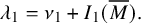 $$ \begin{align} \lambda_1 = \nu_1 + I_1(\overline{M}). \end{align} $$
In [Reference Betea, Bouttier, Nejjar and Vuletić10, Theorem 2.1], authors prove a similar statement relating the first row ( $\lambda _1$
) of a ‘free boundary Schur processes’ to a random shift (
$\lambda _1$
) of a ‘free boundary Schur processes’ to a random shift ( $\nu _1$
) of the last passage time
$\nu _1$
) of the last passage time $I_1$
in a geometry slightly different from the cylinder
$I_1$
in a geometry slightly different from the cylinder $\mathscr {C}_n$
. Such statement follows from standard properties of Fomin growth diagrams and in [Reference Betea, Bouttier, Nejjar and Vuletić10] the quantity
$\mathscr {C}_n$
. Such statement follows from standard properties of Fomin growth diagrams and in [Reference Betea, Bouttier, Nejjar and Vuletić10] the quantity $I_1$
was just the last passage time and it was not related to the asymptotic increment of the corresponding pair
$I_1$
was just the last passage time and it was not related to the asymptotic increment of the corresponding pair $(P,Q)$
. Proposition 1.2 and this corollary represent a partial answer to questions (1) and (3) of [Reference Sagan and Stanley73, Section 9].
$(P,Q)$
. Proposition 1.2 and this corollary represent a partial answer to questions (1) and (3) of [Reference Sagan and Stanley73, Section 9].
To prove Proposition 1.2, we regard fillings of the twisted cylinder $\mathscr {C}_n$
as ‘particle’ configurations. We then define a deterministic dynamics
$\mathscr {C}_n$
as ‘particle’ configurations. We then define a deterministic dynamics $\mathbf {V}:\overline {M} \mapsto \overline {M}'$
, transporting particles from sources of Viennot’s shadow lines to the sinks. For the definition of the map
$\mathbf {V}:\overline {M} \mapsto \overline {M}'$
, transporting particles from sources of Viennot’s shadow lines to the sinks. For the definition of the map $\mathbf {V}$
, see Proposition 4.6, while for a quick view of rules of this dynamics see Figure 11 at page in the text, where sources (resp. sinks) are denoted as black (resp. red) dots. This Viennot dynamics is, in a sense, ‘dual’ to the skew
$\mathbf {V}$
, see Proposition 4.6, while for a quick view of rules of this dynamics see Figure 11 at page in the text, where sources (resp. sinks) are denoted as black (resp. red) dots. This Viennot dynamics is, in a sense, ‘dual’ to the skew $\mathbf {RSK}$
dynamics, but conservation laws are more transparent in this picture. Indeed, we will show, in Proposition 6.5 below, that last passage times are conserved quantities, that is,
$\mathbf {RSK}$
dynamics, but conservation laws are more transparent in this picture. Indeed, we will show, in Proposition 6.5 below, that last passage times are conserved quantities, that is, $I_k(\overline {M}) = I_k(\overline {M}')$
holds. To prove this, we will utilize a number of well-known relations between insertion algorithms and other common operations in combinatorics, as the jeu de taquin, Knuth relations, Kashiwara operators and so on. For the sake of clarity of the exposition these prerequisites will be covered, although not extensively, in Section 5 and Appendix A. Translating this into the language of the skew
$I_k(\overline {M}) = I_k(\overline {M}')$
holds. To prove this, we will utilize a number of well-known relations between insertion algorithms and other common operations in combinatorics, as the jeu de taquin, Knuth relations, Kashiwara operators and so on. For the sake of clarity of the exposition these prerequisites will be covered, although not extensively, in Section 5 and Appendix A. Translating this into the language of the skew $\mathbf {RSK}$
dynamics leads to the proof of Proposition 1.2.
$\mathbf {RSK}$
dynamics leads to the proof of Proposition 1.2.
1.3.2 The bijection $\Upsilon $
: statement of results
$\Upsilon $
: statement of results

We come now to present the main result of this paper: a bijection between pairs of semistandard tableaux and pairs of vertically strict tableaux equipped with additional weights. For any partition $\mu $
, we define the set
$\mu $
, we define the set
 $$ \begin{align} \mathcal{K}(\mu) = \{ \kappa=(\kappa_1,\dots,\kappa_{\mu_1}) \in \mathbb{N}_0^{\mu_1} : \kappa_i\ge \kappa_{i+1} \text{ if } \mu_{i}^{\prime} = \mu_{i+1}^{\prime} \} \end{align} $$
and for any list of nonnegative integers $\eta $
, we denote
$\eta $
, we denote $|\eta |=\eta _1+\eta _2+\cdots $
.
$|\eta |=\eta _1+\eta _2+\cdots $
.
Theorem 1.4 (Proposition 8.1 in the text).
There exists a bijection
![]() between the set of pairs
between the set of pairs $(P,Q)$
of semistandard Young tableaux with the same skew shape and quadruples
$(P,Q)$
of semistandard Young tableaux with the same skew shape and quadruples $(V,W;\kappa ;\nu )$
, with the following properties:
$(V,W;\kappa ;\nu )$
, with the following properties:
-
(i)
$V,W$
are a pair of vertically strict tableaux of shape
$\mu $
and
$\Phi (P,Q)=(V,W)$
; -
(ii)
$\kappa \in \mathcal {K}(\mu )$
and
$\nu $
is a partition; -
(iii) if
$P,Q$
have skew shape
$\lambda /\rho $
, then (1.23)where
$$ \begin{align} |\rho| = \mathscr{H}(V) + \mathscr{H}(W) + |\kappa| + |\nu|, \end{align} $$
$\mathscr {H}$
is the intrinsic energy function; see Proposition 7.4 in the text.


Note that composing $\Upsilon $
with the Sagan–Stanley correspondence allows to factor out the partition
$\Upsilon $
with the Sagan–Stanley correspondence allows to factor out the partition $\nu $
yielding a bijection, denoted by
$\nu $
yielding a bijection, denoted by $\tilde {\Upsilon }$
, between matrices
$\tilde {\Upsilon }$
, between matrices $\overline {M}$
and triples
$\overline {M}$
and triples $(V,W;\kappa )$
. This is more similar to the classical RSK correpondence; see Proposition 8.2.
$(V,W;\kappa )$
. This is more similar to the classical RSK correpondence; see Proposition 8.2.
Equality (1.23) represents the most nontrivial property of $\Upsilon $
. The intrinsic energy
$\Upsilon $
. The intrinsic energy $\mathscr {H}$
, discussed more in Section 1.3.3 and at length in Section 7.1, is a grading statistic on the set of vertically strict tableaux, which was originally introduced in the theory of crystals [Reference Hatayama, Kuniba, Okado, Takagi and Tsuboi41, Reference Nakayashiki and Yamada65, Reference Okado, Schilling and Shimozono67]. Its precise definition requires the notion of combinatorial R-matrix and is not reported here in the introduction, but morally it measures how much a vertically strict tableaux needs to be ‘modified’ to produce a semistandard tableaux.
$\mathscr {H}$
, discussed more in Section 1.3.3 and at length in Section 7.1, is a grading statistic on the set of vertically strict tableaux, which was originally introduced in the theory of crystals [Reference Hatayama, Kuniba, Okado, Takagi and Tsuboi41, Reference Nakayashiki and Yamada65, Reference Okado, Schilling and Shimozono67]. Its precise definition requires the notion of combinatorial R-matrix and is not reported here in the introduction, but morally it measures how much a vertically strict tableaux needs to be ‘modified’ to produce a semistandard tableaux.
Although the algorithmic definition of the skew $\mathbf {RSK}$
dynamics is not very complicated to apply to specific examples, as we did in Section 1.2, proving its various properties using only the defining rules poses serious difficulties. To circumvent these issues, we will implement a more powerful machinery based on symmetries. More precisely, we will show that the skew
$\mathbf {RSK}$
dynamics is not very complicated to apply to specific examples, as we did in Section 1.2, proving its various properties using only the defining rules poses serious difficulties. To circumvent these issues, we will implement a more powerful machinery based on symmetries. More precisely, we will show that the skew $\mathbf {RSK}$
dynamics possesses an affine bicrystal symmetry associated with the affine Lie algebra
$\mathbf {RSK}$
dynamics possesses an affine bicrystal symmetry associated with the affine Lie algebra $\widehat {\mathfrak {sl}}_n$
. This will allow us to linearize the dynamics, resulting in the precise construction of bijection
$\widehat {\mathfrak {sl}}_n$
. This will allow us to linearize the dynamics, resulting in the precise construction of bijection $\Upsilon $
and in the proof of its various properties.
$\Upsilon $
and in the proof of its various properties.
1.3.3 Crystal structure
In order to establish Proposition 1.4, we import ideas from the theory of crystals [Reference Bump and Schilling16, Reference Hong and Kang42], which was introduced by Kashiwara and Lusztig [Reference Kashiwara49, Reference Kashiwara50, Reference Lusztig61] to study representations of quantum groups. In this paper, we will only deal with the simple case of the affine Lie algebra $\widehat {\mathfrak {sl}}_n$
. Applications of crystals are also common in the context of the BBS, which was mentioned after Question 1 in Section 1.2. For example, conserved quantities, scattering rules and phase shifts of the BBS can be studied using affine crystals [Reference Fukuda, Okado and Yamada30, Reference Inoue, Kuniba and Takagi46]. We will apply these ideas to precisely analyze the skew
$\widehat {\mathfrak {sl}}_n$
. Applications of crystals are also common in the context of the BBS, which was mentioned after Question 1 in Section 1.2. For example, conserved quantities, scattering rules and phase shifts of the BBS can be studied using affine crystals [Reference Fukuda, Okado and Yamada30, Reference Inoue, Kuniba and Takagi46]. We will apply these ideas to precisely analyze the skew $\mathbf {RSK}$
dynamics.
$\mathbf {RSK}$
dynamics.
Many of the combinatorial objects we deal with possess a natural crystal structure. For instance, it is a well-known fact that many properties of the RSK correspondence can be understood in the language of $\mathfrak {sl}_n$
crystals [Reference Bump and Schilling16, Reference Lothaire60]. In fact, as recalled in [Reference Shimozono81], even the original algorithm by Robinson [Reference Robinson72], could be stated in terms of crystals. The idea, implicit in [Reference Robinson72], is to assign a permutation
$\mathfrak {sl}_n$
crystals [Reference Bump and Schilling16, Reference Lothaire60]. In fact, as recalled in [Reference Shimozono81], even the original algorithm by Robinson [Reference Robinson72], could be stated in terms of crystals. The idea, implicit in [Reference Robinson72], is to assign a permutation $\pi $
to a pair of tableaux in such a way that the assignment commutes with certain transformations, which are nothing but Kashiwara operators
$\pi $
to a pair of tableaux in such a way that the assignment commutes with certain transformations, which are nothing but Kashiwara operators $\widetilde {e}_{i},\widetilde {f}_{i},i=1,\dots ,n-1$
in today’s language. Kashiwara operators act on a word by changing its content according to certain rules; for instance,
$\widetilde {e}_{i},\widetilde {f}_{i},i=1,\dots ,n-1$
in today’s language. Kashiwara operators act on a word by changing its content according to certain rules; for instance, $\widetilde {e}_{i}$
would change a letter
$\widetilde {e}_{i}$
would change a letter $i+1$
into i, see Section 5.2. In this way, starting from
$i+1$
into i, see Section 5.2. In this way, starting from $\pi $
, through successive applications of
$\pi $
, through successive applications of $\widetilde {e}_{i},\widetilde {f}_{i}$
one would transform it into a Yamanouchi word
$\widetilde {e}_{i},\widetilde {f}_{i}$
one would transform it into a Yamanouchi word $\pi _{\mathrm {Yam}}$
whose corresponding tableaux are canonically determined. Then to deduce the pair
$\pi _{\mathrm {Yam}}$
whose corresponding tableaux are canonically determined. Then to deduce the pair $(P,Q)$
associated to
$(P,Q)$
associated to $\pi $
one would apply in reverse order the inverse of each Kashiwara operator, whose corresponding action on tableaux is defined through their column reading word (see Section 5.2).
$\pi $
one would apply in reverse order the inverse of each Kashiwara operator, whose corresponding action on tableaux is defined through their column reading word (see Section 5.2).
An example of a well-known $\widehat {\mathfrak {sl}}_n$
crystals, which is relevant for our discussions, is the one of vertically strict tableaux. Here, in addition to
$\widehat {\mathfrak {sl}}_n$
crystals, which is relevant for our discussions, is the one of vertically strict tableaux. Here, in addition to $\widetilde {e}_{i},\widetilde {f}_{i}$
with
$\widetilde {e}_{i},\widetilde {f}_{i}$
with $i=1,\dots , n-1$
one has to consider two more operators
$i=1,\dots , n-1$
one has to consider two more operators $\widetilde {e}_{0},\widetilde {f}_{0}$
, which act by replacing
$\widetilde {e}_{0},\widetilde {f}_{0}$
, which act by replacing $1$
-labels into n-labels and vice versa, and they are defined conjugating
$1$
-labels into n-labels and vice versa, and they are defined conjugating $\widetilde {e}_{1},\widetilde {f}_{1}$
by an operation called promotion [Reference Shimozono80]. On the set of pairs of vertically strict tableaux
$\widetilde {e}_{1},\widetilde {f}_{1}$
by an operation called promotion [Reference Shimozono80]. On the set of pairs of vertically strict tableaux $(V,W)$
, we may define two commuting families of Kashiwara operators
$(V,W)$
, we may define two commuting families of Kashiwara operators
 $$ \begin{align} \widetilde{E}_i^{(1)} = \widetilde{e}_{i} \times \mathbf{1}, \qquad \widetilde{E}_i^{(2)} = \mathbf{1} \times \widetilde{e}_{i}, \qquad \widetilde{F}_i^{(1)} = \widetilde{f}_{i} \times \mathbf{1}, \qquad \widetilde{F}_i^{(2)} = \mathbf{1} \times \widetilde{f}_{i}, \end{align} $$
letting $\widetilde {e}_{i},\widetilde {f}_{i}$
act on single components, and this defines an example of
$\widetilde {e}_{i},\widetilde {f}_{i}$
act on single components, and this defines an example of $\widehat {\mathfrak {sl}}_n$
bicrystal.
$\widehat {\mathfrak {sl}}_n$
bicrystal.
To study the skew $\mathbf {RSK}$
dynamics, we want to equip also the space of pairs
$\mathbf {RSK}$
dynamics, we want to equip also the space of pairs $(P,Q)$
of semistandard tableaux of skew shape with an
$(P,Q)$
of semistandard tableaux of skew shape with an $\widehat {\mathfrak {sl}}_n$
bicrystal structure, with the requirement that projection
$\widehat {\mathfrak {sl}}_n$
bicrystal structure, with the requirement that projection $\Phi :(P,Q)\mapsto (V,W)$
commutes with the action of respective Kashiwara operators. It turns out, however, that a naive action of Kashiwara operators
$\Phi :(P,Q)\mapsto (V,W)$
commutes with the action of respective Kashiwara operators. It turns out, however, that a naive action of Kashiwara operators $\widetilde {e}_{i},\widetilde {f}_{i}$
used above for vertically strict tableaux is not appropriate on skew tableaux. This is because, while
$\widetilde {e}_{i},\widetilde {f}_{i}$
used above for vertically strict tableaux is not appropriate on skew tableaux. This is because, while $\widetilde {E}_i^{(\epsilon )}, \widetilde {F}_i^{(\epsilon )}$
for
$\widetilde {E}_i^{(\epsilon )}, \widetilde {F}_i^{(\epsilon )}$
for $i=1,\dots , n-1$
and
$i=1,\dots , n-1$
and $\epsilon =1,2$
commute with the skew
$\epsilon =1,2$
commute with the skew $\mathbf {RSK}$
map, the same is not true for the 0-th operators
$\mathbf {RSK}$
map, the same is not true for the 0-th operators $\widetilde {E}_0^{(\epsilon )}, \widetilde {F}_0^{(\epsilon )}$
. One of the key novelties in this paper is that the desired 0-th Kashiwara operators, which commute with the skew
$\widetilde {E}_0^{(\epsilon )}, \widetilde {F}_0^{(\epsilon )}$
. One of the key novelties in this paper is that the desired 0-th Kashiwara operators, which commute with the skew $\mathbf {RSK}$
map and make of
$\mathbf {RSK}$
map and make of $\Phi $
a morphism of bicrystal graphs in the sense of Proposition 5.1, can be defined using the operation
$\Phi $
a morphism of bicrystal graphs in the sense of Proposition 5.1, can be defined using the operation $\iota _2$
. As a result, they will act nontrivially on both tableaux of the pair
$\iota _2$
. As a result, they will act nontrivially on both tableaux of the pair $(P,Q)$
. They are given by
$(P,Q)$
. They are given by
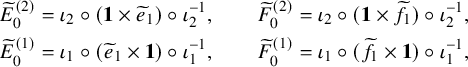 $$ \begin{align} \begin{aligned}\widetilde{E}_0^{(2)} &= \iota_2 \circ ( \mathbf{1} \times \widetilde{e}_{1} ) \circ \iota_2^{-1},\qquad \widetilde{F}_0^{(2)} = \iota_2 \circ ( \mathbf{1} \times \widetilde{f}_{1} ) \circ \iota_2^{-1},\\\widetilde{E}_0^{(1)} &= \iota_1 \circ ( \widetilde{e}_{1} \times \mathbf{1} ) \circ \iota_1^{-1}, \qquad \widetilde{F}_0^{(1)} = \iota_1 \circ ( \widetilde{f}_{1} \times \mathbf{1} ) \circ \iota_1^{-1},\end{aligned} \end{align} $$
where $\iota _1$
is defined through
$\iota _1$
is defined through $\iota _2$
inverting roles of
$\iota _2$
inverting roles of $P,Q$
, that is
$P,Q$
, that is $\iota _1(P,Q) = \mathrm {swap} \circ \iota _2 \circ \mathrm {swap} (P,Q)$
. Here,
$\iota _1(P,Q) = \mathrm {swap} \circ \iota _2 \circ \mathrm {swap} (P,Q)$
. Here, $\mathrm {swap}$
is defined by
$\mathrm {swap}$
is defined by $\mathrm {swap}(P,Q)=(Q,P)$
. In this way, as we will show in Section 5.4, the set of pairs of semistandard tableaux possess an
$\mathrm {swap}(P,Q)=(Q,P)$
. In this way, as we will show in Section 5.4, the set of pairs of semistandard tableaux possess an $\widehat {\mathfrak {sl}}_n$
bicrystal structure.
$\widehat {\mathfrak {sl}}_n$
bicrystal structure.
1.3.4 The bijection
$\Upsilon $
: construction

With these preparations, we may now precisely define the correspondence $\Upsilon $
of Proposition 1.4. For this, we study the skew
$\Upsilon $
of Proposition 1.4. For this, we study the skew $\mathbf {RSK}$
dynamics for a generic tableaux
$\mathbf {RSK}$
dynamics for a generic tableaux $(P,Q)$
by generalizing the idea by Robinson. Namely, we first bring the pair
$(P,Q)$
by generalizing the idea by Robinson. Namely, we first bring the pair $(P,Q)$
into a certain canonical form
$(P,Q)$
into a certain canonical form
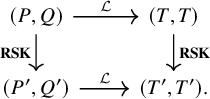
 $(T,T)$
through the action of affine crystal operators, then we run the dynamics on such canonical pair, and finally transforms the result back applying inverse crystal transformations. Schematically, this procedure is summarized by the following commuting diagram.
$(T,T)$
through the action of affine crystal operators, then we run the dynamics on such canonical pair, and finally transforms the result back applying inverse crystal transformations. Schematically, this procedure is summarized by the following commuting diagram.
Here, $(T,T)$
is a pair of identical skew tableaux consisting of generalizations in skew setting of Yamanouchi tableaux.Footnote
3
In the text, we will call them leading tableaux; see Proposition 7.15. The definition of the canonical transformation
$(T,T)$
is a pair of identical skew tableaux consisting of generalizations in skew setting of Yamanouchi tableaux.Footnote
3
In the text, we will call them leading tableaux; see Proposition 7.15. The definition of the canonical transformation $\mathcal {L}$
is delicate and owes to deep results in the theory of affine crystals. If V is a vertically strict tableau with intrinsic energy
$\mathcal {L}$
is delicate and owes to deep results in the theory of affine crystals. If V is a vertically strict tableau with intrinsic energy $\mathscr {H}(V)$
, then a result of [Reference Schilling and Tingley77] guarantees that through the action of Kashiwara operators
$\mathscr {H}(V)$
, then a result of [Reference Schilling and Tingley77] guarantees that through the action of Kashiwara operators $\widetilde {e}_{i},\widetilde {f}_{i}$
one can always transform V into a Yamanouchi tableau of the same shape in such a way that the difference
$\widetilde {e}_{i},\widetilde {f}_{i}$
one can always transform V into a Yamanouchi tableau of the same shape in such a way that the difference $\# \widetilde {f}_{0} - \# \widetilde {e}_{0}$
of 0-th operators used equals
$\# \widetilde {f}_{0} - \# \widetilde {e}_{0}$
of 0-th operators used equals $\mathscr {H}(V)$
. We call such transformation a leading map
$\mathscr {H}(V)$
. We call such transformation a leading map $\mathcal {L}_V$
, and in Section 7.2 we construct it in terms of the so-called Demazure arrows. When
$\mathcal {L}_V$
, and in Section 7.2 we construct it in terms of the so-called Demazure arrows. When $V,W$
are the vertically strict tableaux corresponding to
$V,W$
are the vertically strict tableaux corresponding to $P,Q$
, that is, when
$P,Q$
, that is, when $(V,W)=\Phi (P,Q)$
, they can be both transformed into the same Yamanouchi tableau. For instance, the ones of equation (1.15) are transformed to
$(V,W)=\Phi (P,Q)$
, they can be both transformed into the same Yamanouchi tableau. For instance, the ones of equation (1.15) are transformed to

and the respective leading maps are given by the slightly complicated expressions
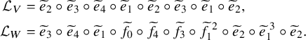 $$ \begin{align} \begin{aligned}\mathcal{L}_{V} &= \widetilde{e}_{2} \circ \widetilde{e}_{3} \circ \widetilde{e}_{4} \circ \widetilde{e}_{1} \circ \widetilde{e}_{2} \circ \widetilde{e}_{3} \circ \widetilde{e}_{1} \circ \widetilde{e}_{2}, \\ \mathcal{L}_{W} &= \widetilde{e}_{3} \circ \widetilde{e}_{4} \circ \widetilde{e}_{1} \circ \widetilde{f}_{0} \circ \widetilde{f}_{4} \circ \widetilde{f}_{3} \circ \widetilde{f}_{1}^{\,\, 2} \circ \widetilde{e}_{2} \circ \widetilde{e}_{1}^{\,\, 3} \circ \widetilde{e}_{2}.\end{aligned} \end{align} $$
Using the affine bicrystal structure for $(P,Q)$
, which is homomorphic to the one for
$(P,Q)$
, which is homomorphic to the one for $(V,W)$
, we can simultaneously lift up the leading maps
$(V,W)$
, we can simultaneously lift up the leading maps $\mathcal {L}_V,\mathcal {L}_W$
and define the map
$\mathcal {L}_V,\mathcal {L}_W$
and define the map $\mathcal {L}$
on
$\mathcal {L}$
on $(P,Q)$
. Moreover, our new 0-th operators (1.25) allow to transport the result of [Reference Schilling and Tingley77] at the level of pairs of skew tableaux.
$(P,Q)$
. Moreover, our new 0-th operators (1.25) allow to transport the result of [Reference Schilling and Tingley77] at the level of pairs of skew tableaux.
In particular, the variation in intrinsic energy at the level of vertically strict tableaux yields the removal of $\mathscr {H}(V) + \mathscr {H}(W)$
empty boxes from the skew shape of
$\mathscr {H}(V) + \mathscr {H}(W)$
empty boxes from the skew shape of $(P,Q)$
. In the text, we will call such map
$(P,Q)$
. In the text, we will call such map $\mathcal {L}$
the leading map of the pair
$\mathcal {L}$
the leading map of the pair $(P,Q)$
. To give an idea of the result of the application of a leading map we consider the pair
$(P,Q)$
. To give an idea of the result of the application of a leading map we consider the pair $(P,Q)$
of equation (1.7), and we have
$(P,Q)$
of equation (1.7), and we have
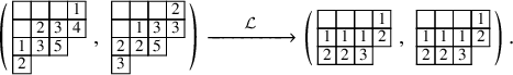
For more details, consult Section 5 and Section 7 in the text. From the computation above, one can observe how the value $\mathscr {H}(V)+\mathscr {H}(W)=1$
, which follows from equation (1.28) counting the number of
$\mathscr {H}(V)+\mathscr {H}(W)=1$
, which follows from equation (1.28) counting the number of $\widetilde {f}_{0}$
operators, coincides with the size difference between skew shapes in equation (1.29).
$\widetilde {f}_{0}$
operators, coincides with the size difference between skew shapes in equation (1.29).
The leading tableau T resulting from the application of a leading map $\mathcal {L}$
, as we will prove in Section 7.4, turns out to be uniquely characterized by a triple of data
$\mathcal {L}$
, as we will prove in Section 7.4, turns out to be uniquely characterized by a triple of data $(\mu ,\kappa ;\nu )$
. Here,
$(\mu ,\kappa ;\nu )$
. Here, $\mu $
is a partition recording the content of T and it is equal to the shape of
$\mu $
is a partition recording the content of T and it is equal to the shape of $V,W$
.
$V,W$
. $\nu $
is also a partition and it can be easily determined by ‘squeezing’ T, that is, moving its rows as much as possible to the left without breaking the semistandard property; see Section 2.4. Finally,
$\nu $
is also a partition and it can be easily determined by ‘squeezing’ T, that is, moving its rows as much as possible to the left without breaking the semistandard property; see Section 2.4. Finally, $\kappa $
is an element of
$\kappa $
is an element of $\mathcal {K}(\mu )$
, and it encodes the empty shape of T after the removal of
$\mathcal {K}(\mu )$
, and it encodes the empty shape of T after the removal of $\nu $
. For the tableau T in the right-hand side of equation (1.29), we have
$\nu $
. For the tableau T in the right-hand side of equation (1.29), we have $\nu =\varnothing $
and
$\nu =\varnothing $
and $\kappa =(0,1,1,1)$
.
$\kappa =(0,1,1,1)$
.
A crucial observation that motivates such a long construction is that, on leading tableaux, the effect of the skew $\mathbf {RSK}$
map becomes purely linear and it modifies the tableaux
$\mathbf {RSK}$
map becomes purely linear and it modifies the tableaux $T(\mu ,\kappa ;\nu )$
by just adding
$T(\mu ,\kappa ;\nu )$
by just adding $\mu '$
to
$\mu '$
to $\kappa $
as
$\kappa $
as
 $$ \begin{align} T=T(\mu,\kappa;\nu) \xrightarrow[]{\hspace{.5cm} \mathbf{RSK} \hspace{.5cm}} T'=T(\mu,\kappa+\mu';\nu). \end{align} $$
The reader familiar with discrete integrable systems might notice that the linearization given by map $\mathcal {L}$
resembles the Kerov–Kirillov–Reshetikhin (KKR) algorithm for BBS [Reference Kuniba, Okado, Sakamoto, Takagi and Yamada56], although the precise connections will be explored in future works.
$\mathcal {L}$
resembles the Kerov–Kirillov–Reshetikhin (KKR) algorithm for BBS [Reference Kuniba, Okado, Sakamoto, Takagi and Yamada56], although the precise connections will be explored in future works.
This parameterization of the leading tableau $T=T(\mu ,\kappa ;\nu )$
, along with the pair
$T=T(\mu ,\kappa ;\nu )$
, along with the pair $(V,W)$
completes the construction of bijection
$(V,W)$
completes the construction of bijection $\Upsilon $
. Notice that equality (1.23) can be understood by carefully analyzing the change of number of empty boxes at each step in the description.
$\Upsilon $
. Notice that equality (1.23) can be understood by carefully analyzing the change of number of empty boxes at each step in the description.
Concluding the example considered throughout the section, we write
1.3.5 Summation identities
Finally, we present some of the immediate consequences of Proposition 1.4. We use the well-known fact [Reference Nakayashiki and Yamada65, Reference Sanderson75, Reference Schilling and Tingley77] that the generating function of vertically strict tableaux of assigned shape $\mu $
and weighted by
$\mu $
and weighted by $\mathscr {H}$
is the q-Whittaker polynomial
$\mathscr {H}$
is the q-Whittaker polynomial
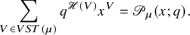 $$ \begin{align} \sum_{V \in VST (\mu)} q^{\mathscr{H}(V)} x^V = \mathscr{P}_{\mu} (x;q). \end{align} $$
Bijection $\Upsilon $
, or more precisely the one between
$\Upsilon $
, or more precisely the one between $\overline {M}$
and
$\overline {M}$
and $(V,W,\kappa )$
mentioned below in Proposition 1.4, allows us to establish the Cauchy identity for q-Whittaker polynomials (1.3).
$(V,W,\kappa )$
mentioned below in Proposition 1.4, allows us to establish the Cauchy identity for q-Whittaker polynomials (1.3).
Theorem 1.5 (Bijective proof of Cauchy identity for q-Whittaker polynomials).
Fix $|q|<1$
and the set of variables
$|q|<1$
and the set of variables $x=(x_1,\dots ,x_n)$
,
$x=(x_1,\dots ,x_n)$
, $y=(y_1,\dots ,y_n)$
such that
$y=(y_1,\dots ,y_n)$
such that $|x_iy_j|<1$
. Then equation (1.3) holds and the normalization term is
$|x_iy_j|<1$
. Then equation (1.3) holds and the normalization term is
![]() .
.
The proof of Proposition 1.5 follows a simple bijective argument. The correspondence
![]() introduced below Proposition 1.4 allows one to interpret monomials (in x’s, y’s and q) from the expansion in the right-hand side of equation (1.3), which are parameterized by matrices of sequences
introduced below Proposition 1.4 allows one to interpret monomials (in x’s, y’s and q) from the expansion in the right-hand side of equation (1.3), which are parameterized by matrices of sequences $\overline {M}$
, as monomials in the left-hand side of equation (1.3), which are parameterized by triples
$\overline {M}$
, as monomials in the left-hand side of equation (1.3), which are parameterized by triples $(V,W,\kappa )$
. The full argument is reported in Proposition 10.2, where instead of matrices
$(V,W,\kappa )$
. The full argument is reported in Proposition 10.2, where instead of matrices $\overline {M}$
we use their parameterization in ‘weighted biwords’
$\overline {M}$
we use their parameterization in ‘weighted biwords’ $\overline {\pi }$
.
$\overline {\pi }$
.
The following identity, which refines the Cauchy identity for both skew Schur polynomials (1.2) and q-Whittaker polynomials (1.3), was stated and proven in our very recent work [Reference Imamura, Mucciconi and Sasamoto44] using integrable probabilistic techniques.
Theorem 1.6. Fix $|q|<1$
and sets of variables
$|q|<1$
and sets of variables $x=(x_1,\dots ,x_n)$
,
$x=(x_1,\dots ,x_n)$
, $y=(y_1,\dots ,y_n)$
. Then, for all
$y=(y_1,\dots ,y_n)$
. Then, for all $k=0,1,2,\dots $
, we have
$k=0,1,2,\dots $
, we have
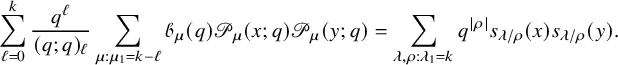
Indeed, the original motivation of this work was to find a bijective proof of this identity, which is now accomplished by the bijection $\Upsilon $
in Proposition 1.4. A number of analogous identities, such as Littlewood-like identities involving summations of single q-Whittaker polynomials, will be presented in Sections 10.1 and 10.2. They all follow from Proposition 1.4 and can be proven bijectively. See Proposition 10.3.
$\Upsilon $
in Proposition 1.4. A number of analogous identities, such as Littlewood-like identities involving summations of single q-Whittaker polynomials, will be presented in Sections 10.1 and 10.2. They all follow from Proposition 1.4 and can be proven bijectively. See Proposition 10.3.
Remark 1.7. The summation identities of Proposition 1.6, as well as equations (1.2), (1.3), have been reported by assuming that the set of variables $x,y$
are n-tuples of complex numbers. Such assumption is not necessary to our results and only serves the purpose of keeping the notation as simple as possible. In general x and y in equation (1.33) can be arbitrary specializations of the algebra of symmetric functions; see Proposition 10.8. Analogously, we have assumed that matrices
$x,y$
are n-tuples of complex numbers. Such assumption is not necessary to our results and only serves the purpose of keeping the notation as simple as possible. In general x and y in equation (1.33) can be arbitrary specializations of the algebra of symmetric functions; see Proposition 10.8. Analogously, we have assumed that matrices $\overline {M}_{i,j}(k)$
are squared; that is,
$\overline {M}_{i,j}(k)$
are squared; that is, $i,j \in \{1,\dots ,n\}$
. This is also not necessary, and our results and constructions hold also for rectangular matrices.
$i,j \in \{1,\dots ,n\}$
. This is also not necessary, and our results and constructions hold also for rectangular matrices.
Identities such as equation (1.33) or equation (10.38) in the text have important consequences in the realm of integrable probability which we will develop in a forthcoming paper [Reference Imamura, Mucciconi and Sasamoto45]. In fact, they provide a new way of solving stochastic integrable systems in the KPZ class connecting q-Whittaker polynomials with manifestly determinantal and pfaffian point processes, as the ones related to skew Schur polynomials [Reference Betea and Bouttier9–Reference Borodin11]. This accomplishes a generalization in q-deformed setting of the original techniques employed by Johansson to solve the totally asymmetric simple exclusion process [Reference Johansson47]. Moreover, properties of bijection $\Upsilon $
, resulting in identity (10.38), allow us to generalize ideas of Baik and Rains who used symmetries of the RSK correspondence to study, on the same footing, asymptotics of random permutations with various symmetries [Reference Baik and Rains5, Reference Baik and Rains6]. In particular, this will solve, bypassing complicated Bethe Ansatz calculations, the outstanding problem of rigorously establishing pfaffian formulas for solvable models in the KPZ class in restricted environment [Reference Barraquand, Borodin and Corwin7, Reference Barraquand, Borodin, Corwin and Wheeler8, Reference Borodin, Bufetov and Corwin12, Reference Krajenbrink and Le Doussal55]. We will elaborate on these results in [Reference Imamura, Mucciconi and Sasamoto45].
$\Upsilon $
, resulting in identity (10.38), allow us to generalize ideas of Baik and Rains who used symmetries of the RSK correspondence to study, on the same footing, asymptotics of random permutations with various symmetries [Reference Baik and Rains5, Reference Baik and Rains6]. In particular, this will solve, bypassing complicated Bethe Ansatz calculations, the outstanding problem of rigorously establishing pfaffian formulas for solvable models in the KPZ class in restricted environment [Reference Barraquand, Borodin and Corwin7, Reference Barraquand, Borodin, Corwin and Wheeler8, Reference Borodin, Bufetov and Corwin12, Reference Krajenbrink and Le Doussal55]. We will elaborate on these results in [Reference Imamura, Mucciconi and Sasamoto45].
1.4 Outline
In Section 2, we fix the notation and introduce different useful parameterizations of Young tableaux and other combinatorial objects. In Section 3, we discuss the skew $\mathbf {RSK}$
map in its various formulations both in terms of the insertion algorithms and of edge local rules. In Section 4, we describe Sagan and Stanley’s correspondence and we introduce an integrable dynamics on matrices. We call it Viennot dynamics, being based on the shadow line construction. In Section 5, we endow various combinatorial objects with an affine bicrystal structure. In Section 6, we establish conservation laws for the Viennot dynamics and characterize asymptotic increments
$\mathbf {RSK}$
map in its various formulations both in terms of the insertion algorithms and of edge local rules. In Section 4, we describe Sagan and Stanley’s correspondence and we introduce an integrable dynamics on matrices. We call it Viennot dynamics, being based on the shadow line construction. In Section 5, we endow various combinatorial objects with an affine bicrystal structure. In Section 6, we establish conservation laws for the Viennot dynamics and characterize asymptotic increments $\mu (P,Q)$
as Greene invariants. In Section 7, we discuss the combinatorial R-matrix, the intrinsic energy function
$\mu (P,Q)$
as Greene invariants. In Section 7, we discuss the combinatorial R-matrix, the intrinsic energy function $\mathscr {H}$
. Subsequently, we implement a combinatorial transformation that reduces the skew
$\mathscr {H}$
. Subsequently, we implement a combinatorial transformation that reduces the skew $\mathbf {RSK}$
map to a linear map. Such linearization defines a useful class of tableaux, we call leading tableaux and which we study in detail. In Section 8, we discuss our bijection
$\mathbf {RSK}$
map to a linear map. Such linearization defines a useful class of tableaux, we call leading tableaux and which we study in detail. In Section 8, we discuss our bijection $\Upsilon $
, proving Proposition 1.4. In Section 8.3, we also propose, without entering technical discussion, a few natural extensions of Proposition 1.4. In Section 9, we study the scattering and phase shift of the skew
$\Upsilon $
, proving Proposition 1.4. In Section 8.3, we also propose, without entering technical discussion, a few natural extensions of Proposition 1.4. In Section 9, we study the scattering and phase shift of the skew $\mathbf {RSK}$
dynamics. Finally, in Section 10, we give proofs of a number of summation identities for q-Whittaker polynomials and skew Schur polynomials. In Appendix A, we review classical notions of Knuth relations and we propose their generalizations in skew setting. In Appendix B, we give a proof of an invariance property of last passage times with respect to crystal operators.
$\mathbf {RSK}$
dynamics. Finally, in Section 10, we give proofs of a number of summation identities for q-Whittaker polynomials and skew Schur polynomials. In Appendix A, we review classical notions of Knuth relations and we propose their generalizations in skew setting. In Appendix B, we give a proof of an invariance property of last passage times with respect to crystal operators.
2 Preliminary notions
2.1 Biwords and matrices of integers
We introduce the alphabet $\mathcal {A}_n=\{1,\dots ,n\}$
, and we denote by
$\mathcal {A}_n=\{1,\dots ,n\}$
, and we denote by $\mathcal {A}_n^*$
the set of word of finite length in
$\mathcal {A}_n^*$
the set of word of finite length in $\mathcal {A}_n$
. The length of a word p is denoted by
$\mathcal {A}_n$
. The length of a word p is denoted by $\ell (p)$
, while its content is recorded by an array
$\ell (p)$
, while its content is recorded by an array $\gamma =(\gamma _1, \dots , \gamma _n)$
, where
$\gamma =(\gamma _1, \dots , \gamma _n)$
, where $\gamma _i$
equals the multiplicity of i in p.
$\gamma _i$
equals the multiplicity of i in p.
Given two natural numbers $n,m$
we denote by
$n,m$
we denote by $\mathbb {A}_{n,m}$
the set of biwords in the alphabets
$\mathbb {A}_{n,m}$
the set of biwords in the alphabets $\mathcal {A}_n, \mathcal {A}_m$
. A biword
$\mathcal {A}_n, \mathcal {A}_m$
. A biword $\pi \in \mathbb {A}_{n,m}$
is an array of pairs
$\pi \in \mathbb {A}_{n,m}$
is an array of pairs $\left (\begin {smallmatrix} q_1 & q_2 & \cdots & q_k \\p_1 &p_2 &\cdots &p_k \end {smallmatrix}\right )$
,
$\left (\begin {smallmatrix} q_1 & q_2 & \cdots & q_k \\p_1 &p_2 &\cdots &p_k \end {smallmatrix}\right )$
, $k\in \mathbb {N}$
, where
$k\in \mathbb {N}$
, where $q_i\in \mathcal {A}_m$
,
$q_i\in \mathcal {A}_m$
, $p_i\in \mathcal {A}_n$
and whose columns are ordered lexicographically. This means that for all i we have
$p_i\in \mathcal {A}_n$
and whose columns are ordered lexicographically. This means that for all i we have $q_i \le q_{i+1}$
and whenever
$q_i \le q_{i+1}$
and whenever $q_i=q_{i+1}$
, then
$q_i=q_{i+1}$
, then $p_i \le p_{i+1}$
. Clearly, words
$p_i \le p_{i+1}$
. Clearly, words $p_1 \dots p_k$
are particular cases of biwords, obtained setting
$p_1 \dots p_k$
are particular cases of biwords, obtained setting $q_i=i$
. Permutations
$q_i=i$
. Permutations $\sigma \in \mathcal {S}_n$
are also particular cases of biwords where we set
$\sigma \in \mathcal {S}_n$
are also particular cases of biwords where we set $q_i=i$
and
$q_i=i$
and $p_i=\sigma _i$
.
$p_i=\sigma _i$
.
Given $\mathcal {A}_n,\mathcal {A}_m$
we consider weighted biwords in these alphabets and we denote their set by
$\mathcal {A}_n,\mathcal {A}_m$
we consider weighted biwords in these alphabets and we denote their set by $\overline {\mathbb {A}}_{n,m}$
. Elements of
$\overline {\mathbb {A}}_{n,m}$
. Elements of $\overline {\mathbb {A}}_{n,m}$
are arrays of tripletsFootnote
4
$\overline {\mathbb {A}}_{n,m}$
are arrays of tripletsFootnote
4
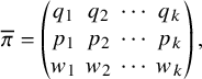 $$ \begin{align} \overline{\pi} = \left(\begin{matrix} q_1 & q_2 & \cdots & q_k \\ p_1 & p_2 & \cdots & p_k \\w_1 & w_2 &\cdots &w_k \end{matrix}\right), \end{align} $$
where again $q_i\in \mathcal {A}_m$
,
$q_i\in \mathcal {A}_m$
, $p_i \in \mathcal {A}_n$
and weights
$p_i \in \mathcal {A}_n$
and weights $w_i \in \mathbb {Z}$
. Columns of a weighted biword are arranged so that the biword composed by
$w_i \in \mathbb {Z}$
. Columns of a weighted biword are arranged so that the biword composed by $q,p$
is lexicographically ordered, with top entries taking precedence, while if
$q,p$
is lexicographically ordered, with top entries taking precedence, while if $q_i=q_{i+1}$
and
$q_i=q_{i+1}$
and $p_i=p_{i+1}$
, then
$p_i=p_{i+1}$
, then $w_i \ge w_{i+1}$
. The total weight of a weighted biword
$w_i \ge w_{i+1}$
. The total weight of a weighted biword $\overline {\pi }$
is the sum of the
$\overline {\pi }$
is the sum of the $w_i$
entries and we denote it by
$w_i$
entries and we denote it by $\mathrm {wt}(\overline {\pi })$
, that is,
$\mathrm {wt}(\overline {\pi })$
, that is, $\mathrm {wt}(\overline {\pi }) = \sum _i w_i$
. In this text, weighted biwords will always be denoted by overlined Greek letters
$\mathrm {wt}(\overline {\pi }) = \sum _i w_i$
. In this text, weighted biwords will always be denoted by overlined Greek letters $\overline {\pi },\overline {\sigma },\overline {\xi },\dots $
so to distinguish them from biwords, whose symbols are never overlined.
$\overline {\pi },\overline {\sigma },\overline {\xi },\dots $
so to distinguish them from biwords, whose symbols are never overlined.
For later use, we also present an alternative format to express a weighted biword, which we call timetable ordering. Given $\overline {\pi }$
its timetable ordering
$\overline {\pi }$
its timetable ordering
![]() is the array consisting of the same triplets of
is the array consisting of the same triplets of $\overline {\pi }$
arranged in such a way that
$\overline {\pi }$
arranged in such a way that
![]() and in case
and in case
![]() then
then
![]() and if also
and if also
![]() then
then
![]() . Examples of a weighted biword and of its timetable ordering are
. Examples of a weighted biword and of its timetable ordering are
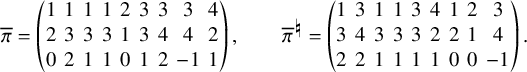
Particular cases of weighted biwords are weighted words, where we assume $q_i=i$
, or weighted permutations, where
$q_i=i$
, or weighted permutations, where $q_i=i$
and
$q_i=i$
and $p_1,\cdots , p_k$
form a permutation of
$p_1,\cdots , p_k$
form a permutation of $\{ 1, \dots , k\}$
. We also use the notion of partial (weighted) permutations, that are weighted biwords where each q and p rows present no repetitions. The set of weighted biwords where all weights are nonnegative integers will be important to us and is denoted with
$\{ 1, \dots , k\}$
. We also use the notion of partial (weighted) permutations, that are weighted biwords where each q and p rows present no repetitions. The set of weighted biwords where all weights are nonnegative integers will be important to us and is denoted with $\overline {\mathbb {A}}_{n,m}^+$
.
$\overline {\mathbb {A}}_{n,m}^+$
.
Biwords of $\mathbb {A}_{n,m}$
are in natural bijection with the set of rectangular matrices with nonnegative integral entries
$\mathbb {A}_{n,m}$
are in natural bijection with the set of rectangular matrices with nonnegative integral entries
Such correspondence is realized assigning to $\pi $
the matrix m with elements
$\pi $
the matrix m with elements
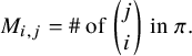 $$ \begin{align} M_{i,j}=\# \text{ of } \binom{j}{i} \text{ in } \pi. \end{align} $$
Analogously, weighted biwords of $\overline {\mathbb {A}}_{n,m}$
are in correspondence with rectangular matrices whose elements are eventually vanishing sequences of nonnegative integers
$\overline {\mathbb {A}}_{n,m}$
are in correspondence with rectangular matrices whose elements are eventually vanishing sequences of nonnegative integers
 $$ \begin{align} \overline{\mathbb{M}}_{n\times m} = \{ (\overline{M}_{i,j}:\mathbb{Z} \to \mathbb{N}_0 : 1\le i \le n, 1 \le j \le m) : \overline{M}_{i,j}(k) = 0 \text{ for } |k| \gg 0 \}. \end{align} $$
Also in this case to a weighted biword $\overline {\pi }$
, we assign the matrix
$\overline {\pi }$
, we assign the matrix $\overline {M}$
defined by
$\overline {M}$
defined by
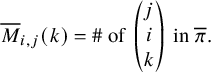 $$ \begin{align} \overline{M}_{i,j}(k) = \# \text{ of } \left( \begin{matrix} j\\i\\k \end{matrix} \right) \text{ in } \overline{\pi}. \end{align} $$
As earlier, we will always denote matrices of $\overline {\mathbb {M}}_{n \times m}$
by overlined capital letters to distinguish them from those of
$\overline {\mathbb {M}}_{n \times m}$
by overlined capital letters to distinguish them from those of $\mathbb {M}_{n \times m}$
. The subset of
$\mathbb {M}_{n \times m}$
. The subset of $\overline {\mathbb {M}}_{n \times m}$
in bijection with nonnegatively weighted biwords
$\overline {\mathbb {M}}_{n \times m}$
in bijection with nonnegatively weighted biwords $\overline {\mathbb {A}}_{n,m}^+$
is denoted by
$\overline {\mathbb {A}}_{n,m}^+$
is denoted by $\overline {\mathbb {M}}_{n \times m}^+$
. The weight of a matrix is defined as
$\overline {\mathbb {M}}_{n \times m}^+$
. The weight of a matrix is defined as
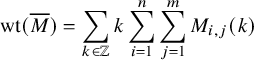 $$ \begin{align*} \mathrm{wt}(\overline{M}) = \sum_{k \in\mathbb{Z}}k \sum_{i=1}^n \sum_{j=1}^m M_{i,j}(k) \end{align*} $$
so that under correspondence (2.6) we have $\mathrm {wt}(\overline {M}) = \mathrm {wt}(\overline {\pi })$
. We will represent matrices
$\mathrm {wt}(\overline {M}) = \mathrm {wt}(\overline {\pi })$
. We will represent matrices $\overline {M}\in \overline {\mathbb {M}}_{n \times m}$
, with a slight abuse of notation, as compactly supported maps
$\overline {M}\in \overline {\mathbb {M}}_{n \times m}$
, with a slight abuse of notation, as compactly supported maps $\overline {M} : \{1, \dots , m\} \times \mathbb {Z} \to \mathbb {N}_0$
via the identification
$\overline {M} : \{1, \dots , m\} \times \mathbb {Z} \to \mathbb {N}_0$
via the identification
 $$ \begin{align} \overline{M}(j,i-kn) = \overline{M}_{i,j}(k), \qquad \text{for all} \qquad i\in \mathcal{A}_n,\, j\in \mathcal{A}_m, \, k\in \mathbb{Z}. \end{align} $$
Given two weighted biwords $\overline {\pi },\overline {\pi }'$
, we consider their disjoint union
$\overline {\pi },\overline {\pi }'$
, we consider their disjoint union
![]() formed taking all columns of
formed taking all columns of $\overline {\pi }$
and
$\overline {\pi }$
and $\overline {\pi }'$
and rearranging them in the correct order. In case
$\overline {\pi }'$
and rearranging them in the correct order. In case $\overline {M},\overline {M}'$
are the matrices corresponding to
$\overline {M},\overline {M}'$
are the matrices corresponding to $\overline {\pi },\overline {\pi }'$
, then naturally
$\overline {\pi },\overline {\pi }'$
, then naturally $\overline {M} + \overline {M}'$
is the matrix associated to their union.
$\overline {M} + \overline {M}'$
is the matrix associated to their union.
Throughout the paper, we will consider a number of operations on biwords and most of times these will have a nice description in the language of matrices. For instance, if $\overline {M}$
is the matrix corresponding to a weighted biword
$\overline {M}$
is the matrix corresponding to a weighted biword $\overline {\pi }$
, then to its transpose
$\overline {\pi }$
, then to its transpose $\overline {M}^T$
it will correspond a biword
$\overline {M}^T$
it will correspond a biword $\overline {\pi }^{-1}$
obtained from
$\overline {\pi }^{-1}$
obtained from $\overline {\pi }$
swapping the p and the q rows and rearranging the result in the prescribed order. This notation is standard and is justified by the fact that when
$\overline {\pi }$
swapping the p and the q rows and rearranging the result in the prescribed order. This notation is standard and is justified by the fact that when $\overline {\pi }$
is a permutation
$\overline {\pi }$
is a permutation $\overline {\pi }^{-1}$
is its inverse in the symmetric group.
$\overline {\pi }^{-1}$
is its inverse in the symmetric group.
2.2 Partitions and Young diagrams
A partition $\lambda =(\lambda _1, \lambda _2,\cdots )$
is a weakly decreasing sequence of integers
$\lambda =(\lambda _1, \lambda _2,\cdots )$
is a weakly decreasing sequence of integers $\lambda _i$
eventually being zero. The number of nonzero parts of
$\lambda _i$
eventually being zero. The number of nonzero parts of $\lambda $
is its length, and it is denoted by
$\lambda $
is its length, and it is denoted by $\ell (\lambda )$
. We say that
$\ell (\lambda )$
. We say that $\lambda $
partitions k if
$\lambda $
partitions k if $| \lambda | = \lambda _1 + \lambda _2 + \cdots = k$
and sometimes we write
$| \lambda | = \lambda _1 + \lambda _2 + \cdots = k$
and sometimes we write $\lambda \vdash k$
. The multiplicative notation
$\lambda \vdash k$
. The multiplicative notation $\lambda =1^{m_1(\lambda )} 2^{m_2(\lambda )}\cdots $
is often used and
$\lambda =1^{m_1(\lambda )} 2^{m_2(\lambda )}\cdots $
is often used and $m_i(\lambda )$
denotes the multiplicity of i in
$m_i(\lambda )$
denotes the multiplicity of i in $\lambda $
. The set of all partitions is denoted by
$\lambda $
. The set of all partitions is denoted by $\mathbb {Y}$
. Sometimes, we will refer to arrays
$\mathbb {Y}$
. Sometimes, we will refer to arrays $\varkappa =(\varkappa _1,\dots ,\varkappa _N) \in \mathbb {N}_0^{N}$
of N nonnegative integers as compositions. Given a composition
$\varkappa =(\varkappa _1,\dots ,\varkappa _N) \in \mathbb {N}_0^{N}$
of N nonnegative integers as compositions. Given a composition $\varkappa \in \mathbb {N}_0^{N}$
, we denote by
$\varkappa \in \mathbb {N}_0^{N}$
, we denote by $\varkappa ^+$
the unique partition that can be generated permuting elements of
$\varkappa ^+$
the unique partition that can be generated permuting elements of $\varkappa $
.
$\varkappa $
.
Partitions are identified by their Young diagrams, and we will freely interchange these two notions. Viewing the plane $\mathbb {Z} \times \mathbb {Z}$
with the vertical coordinate increasing downward, the Young diagram of
$\mathbb {Z} \times \mathbb {Z}$
with the vertical coordinate increasing downward, the Young diagram of $\lambda $
is the collection of cells
$\lambda $
is the collection of cells $(c,r)$
with
$(c,r)$
with $1 \le r \le \ell (\lambda )$
and
$1 \le r \le \ell (\lambda )$
and $1\le c \le \lambda _r$
. Reflecting the Young diagram of
$1\le c \le \lambda _r$
. Reflecting the Young diagram of $\lambda $
with respect to the main diagonal, we obtain the transposed partition
$\lambda $
with respect to the main diagonal, we obtain the transposed partition $\lambda '$
with parts
$\lambda '$
with parts $\lambda _i^{\prime } = \# \{ j: \lambda _j \ge i \}$
. Given two partitions
$\lambda _i^{\prime } = \# \{ j: \lambda _j \ge i \}$
. Given two partitions $\mu , \lambda $
, we write
$\mu , \lambda $
, we write $\mu \subseteq \lambda $
if
$\mu \subseteq \lambda $
if $\mu _i \le \lambda _i$
for all i or equivalently if their Young diagrams are encapsulated. When
$\mu _i \le \lambda _i$
for all i or equivalently if their Young diagrams are encapsulated. When $\mu \subseteq \lambda $
, we define the skew Young diagram
$\mu \subseteq \lambda $
, we define the skew Young diagram $\lambda /\mu $
consisting of all all cells in
$\lambda /\mu $
consisting of all all cells in $\lambda $
but not in
$\lambda $
but not in $\mu $
. The number of cells of
$\mu $
. The number of cells of $\lambda /\mu $
is denoted with
$\lambda /\mu $
is denoted with $|\lambda /\mu |$
.
$|\lambda /\mu |$
.
As hinted in the introduction, for the discussion in this paper, it is essential to allow Young diagrams to have rows at nonpositive coordinates. For this, we define the upward translation $\mathcal {T}_{-i} : (c,r) \mapsto (c,r-i)$
, for any
$\mathcal {T}_{-i} : (c,r) \mapsto (c,r-i)$
, for any $i\in \mathbb {N}_0$
and the set of generalized Young diagrams
$i\in \mathbb {N}_0$
and the set of generalized Young diagrams $\mathbb {Y}_{-i} = \mathcal {T}_{-i} (\mathbb {Y})$
. A generalized Young diagram
$\mathbb {Y}_{-i} = \mathcal {T}_{-i} (\mathbb {Y})$
. A generalized Young diagram $\lambda \in \mathbb {Y}_{-i}$
is associated to its generalized partition
$\lambda \in \mathbb {Y}_{-i}$
is associated to its generalized partition $(\lambda _{1-i},\lambda _{2-i},\dots )$
. The notion of skew diagrams is defined as always: If
$(\lambda _{1-i},\lambda _{2-i},\dots )$
. The notion of skew diagrams is defined as always: If $\mu ,\lambda \in \mathbb {Y}_{-i}$
, then
$\mu ,\lambda \in \mathbb {Y}_{-i}$
, then $\lambda /\mu $
is the set of cells in
$\lambda /\mu $
is the set of cells in $\lambda $
but not in
$\lambda $
but not in $\mu $
. When drawing generalized Young diagrams we will color cells at nonpositive rows in gray to give a reference. We report an example of a skew Young diagram and a generalized one obtained translating it
$\mu $
. When drawing generalized Young diagrams we will color cells at nonpositive rows in gray to give a reference. We report an example of a skew Young diagram and a generalized one obtained translating it
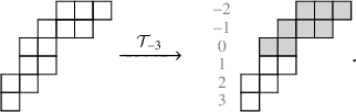
At times, we will need to distinguish generalized Young diagrams from nongeneralized ones, that in these circumstances will be called classical. Statements and constructions reported in this text often apply the same to classical Young diagrams or to generalized Young diagrams and unless required, we will not stress the difference. Nevertheless, we point out that not every operation defined on classical Young diagrams is possible in the generalized case: For instance, the notion of transposition $\lambda '$
is only defined if
$\lambda '$
is only defined if $\lambda \in \mathbb {Y}$
.
$\lambda \in \mathbb {Y}$
.
Given a classical Young diagram $\mu $
, its rectangular decomposition is given by indices
$\mu $
, its rectangular decomposition is given by indices $0=R_0<R_1<\cdots < R_N=\mu _1$
such that
$0=R_0<R_1<\cdots < R_N=\mu _1$
such that
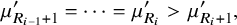 $$ \begin{align} \mu_{R_{i-1}+1}^{\prime} = \cdots = \mu_{R_i}^{\prime}> \mu_{R_i+1}^{\prime}, \end{align} $$
for $i=1,\dots ,N$
; see Figure 3. When using the notion of rectangular decomposition, we will denote by
$i=1,\dots ,N$
; see Figure 3. When using the notion of rectangular decomposition, we will denote by $r_i=R_{i-1}- R_{i}$
the base of each rectangle of
$r_i=R_{i-1}- R_{i}$
the base of each rectangle of $\mu $
.
$\mu $
. $R_i$
’s and
$R_i$
’s and $r_i$
’s for a partition
$r_i$
’s for a partition $\mu $
.
$\mu $
.
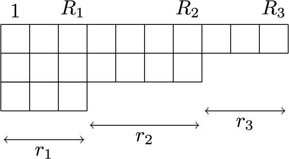
2.3 Young tableaux
A Young tableau, or simply a tableau, T is a filling of cells of a Young diagram with natural numbers. The label assigned to a specific cell $(c,r) \in \lambda $
is indicated with
$(c,r) \in \lambda $
is indicated with $T(c,r)$
and in this case
$T(c,r)$
and in this case $\lambda $
is called shape of T. If a cell has label
$\lambda $
is called shape of T. If a cell has label $\ell $
we call that an
$\ell $
we call that an $\ell $
-cell. The content of a tableau T is recorded by an array
$\ell $
-cell. The content of a tableau T is recorded by an array $\gamma =(\gamma _1,\gamma _2,\dots )$
, where
$\gamma =(\gamma _1,\gamma _2,\dots )$
, where $\gamma _i = \# i$
-cells in T. We will mainly deal with two types of tableaux. Semistandard tableaux have entries strictly increasing column-wise and weakly increasing row-wise. When their labels range in the alphabet
$\gamma _i = \# i$
-cells in T. We will mainly deal with two types of tableaux. Semistandard tableaux have entries strictly increasing column-wise and weakly increasing row-wise. When their labels range in the alphabet $\mathcal {A}_n$
and the shape
$\mathcal {A}_n$
and the shape $\lambda / \rho $
is fixed, we denote their set by
$\lambda / \rho $
is fixed, we denote their set by $SST(\lambda /\rho ,n)$
. In such cases, we call
$SST(\lambda /\rho ,n)$
. In such cases, we call $\lambda $
the external shape and
$\lambda $
the external shape and $\rho $
the empty shape. It could happen that the shape
$\rho $
the empty shape. It could happen that the shape $\lambda /\rho $
of T is a generalized skew Young diagram, as in the examples in Section 1.2, and in such cases T is a generalized semistandard tableau. As before, we will not stress the generalized property unless required. A particular class of semistandard tableaux is that of standard tableaux, defined by the property of having content
$\lambda /\rho $
of T is a generalized skew Young diagram, as in the examples in Section 1.2, and in such cases T is a generalized semistandard tableau. As before, we will not stress the generalized property unless required. A particular class of semistandard tableaux is that of standard tableaux, defined by the property of having content $\gamma _i=1$
for all
$\gamma _i=1$
for all $i=1,\dots , |\lambda / \rho |$
. Their set is denoted by
$i=1,\dots , |\lambda / \rho |$
. Their set is denoted by $ST(\lambda /\rho )$
.
$ST(\lambda /\rho )$
.
The other class of tableaux, which will play an important role in this paper, is that of vertically strict tableaux that have labels strictly increasing column-wise and no additional conditions. These are sometimes called ‘column strict fillings’ [Reference Lenart and Schilling58] or when entries have no repetitions ‘column tabloids’ [Reference Sagan74]. Shapes of vertically strict tableaux will always be straight (i.e., nonskew) classical Young diagrams $\mu \in \mathbb {Y}$
, and we denote their set by
$\mu \in \mathbb {Y}$
, and we denote their set by $VST(\mu ,n)$
when entries range in the alphabet
$VST(\mu ,n)$
when entries range in the alphabet $\mathcal {A}_n$
. Examples of semistandard and vertically strict tableaux are
$\mathcal {A}_n$
. Examples of semistandard and vertically strict tableaux are
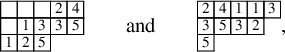
with content, respectively, equal to $(2,2,2,1,2)$
and
$(2,2,2,1,2)$
and $(2,2,3,1,2)$
.
$(2,2,3,1,2)$
.
Given a tableau T, we define its row reading word $\pi ^{\mathrm {row}}_T$
concatenating rows of T starting from the last. Alternatively, the column reading word
$\pi ^{\mathrm {row}}_T$
concatenating rows of T starting from the last. Alternatively, the column reading word $\pi ^{\mathrm {col}}_T$
is formed reading entries of T column by column from the last row up and from left to right. For instance, if T is the semistandard tableau in equation (2.10) we have
$\pi ^{\mathrm {col}}_T$
is formed reading entries of T column by column from the last row up and from left to right. For instance, if T is the semistandard tableau in equation (2.10) we have
 $$ \begin{align} \pi^{\mathrm{row}}_T = 1\,\,2\,\,5\,\,1\,\,3\,\,3\,\,5\,\,2\,\,4 \qquad \textrm{and} \qquad \pi^{\mathrm{col}}_T = 1\,\,2\,\,1\,\,5\,\,3\,\,3\,\,2\,\,5\,\,4. \end{align} $$
2.4 Kernels of tableaux
We now define a useful statistic of a semistandard Young tableau of classical shape.
Definition 2.1. Given a classical skew tableaux $P\in SST(\lambda /\rho ,n)$
, its kernel is the partition
$P\in SST(\lambda /\rho ,n)$
, its kernel is the partition $\varkappa = \ker (P) \in \mathbb {Y}$
such that, for all
$\varkappa = \ker (P) \in \mathbb {Y}$
such that, for all $j=1,2,\dots $
,
$j=1,2,\dots $
, $\varkappa _j - \varkappa _{j+1}$
is the maximal number of boxes one can shift the first j rows of P to the left without breaking the semistandard property.
$\varkappa _j - \varkappa _{j+1}$
is the maximal number of boxes one can shift the first j rows of P to the left without breaking the semistandard property.
For example, if
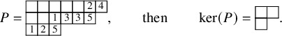
In fact, shifting the second and first row of P, respectively, one and two cells to the left we obtain the semistandard tableau of equation (2.10), which cannot be ‘squeezed’ anymore.
In order to describe more precisely the partition $\ker (P)$
, we introduce the notion of overlap of two weakly increasing words
$\ker (P)$
, we introduce the notion of overlap of two weakly increasing words $A,B$
. This is defined as
$A,B$
. This is defined as $\ell (B)$
minus the size of the empty shape of the minimal semistandard tableaux having first and second row content given by A and B, respectively. In formulas, we have
$\ell (B)$
minus the size of the empty shape of the minimal semistandard tableaux having first and second row content given by A and B, respectively. In formulas, we have
 $$ \begin{align} \mathrm{ov}(A,B) = \max_{L \in \{0,\dots, \ell(A) \wedge \ell(B) \}} \left\{ L : B_{\ell(B)-L+i}> A_{i}, \text{ for all } i=1,\dots,L \right\}. \end{align} $$
For instance, for $A=1 \,\, 3 \,\, 3 \,\, 5$
and
$A=1 \,\, 3 \,\, 3 \,\, 5$
and $B= 1 \,\, 2 \,\, 2 \,\, 3 \,\, 4$
we have
$B= 1 \,\, 2 \,\, 2 \,\, 3 \,\, 4$
we have $\mathrm {ov}(A,B) = 2$
since the minimal semistandard tableaux with first row A and second row B is
$\mathrm {ov}(A,B) = 2$
since the minimal semistandard tableaux with first row A and second row B is
Recording the j-th row of a tableau $P \in SST(\lambda /\rho ,n)$
in a weakly increasing word
$P \in SST(\lambda /\rho ,n)$
in a weakly increasing word $p^{(j)}$
of length
$p^{(j)}$
of length $\theta _j=\lambda _j-\rho _j$
and setting
$\theta _j=\lambda _j-\rho _j$
and setting $\varkappa =\ker (P)$
, we have
$\varkappa =\ker (P)$
, we have
 $$ \begin{align} \varkappa_j - \varkappa_{j+1} = \rho_j - \lambda_{j+1} + \mathrm{ov}(p^{(j)}, p^{(j+1)}). \end{align} $$
Given a pair $(P,Q)$
of semistandard tableaux with the same shape, we can define
$(P,Q)$
of semistandard tableaux with the same shape, we can define $\ker (P,Q)$
in the same way as in Proposition 2.1. If
$\ker (P,Q)$
in the same way as in Proposition 2.1. If $\nu =\ker (P,Q)$
, then
$\nu =\ker (P,Q)$
, then $\nu _j-\nu _{j+1}$
is the maximal amount of cells we can shift the first j rows of P and Q simultaneously to the left without breaking the semistandard property. In this case, if
$\nu _j-\nu _{j+1}$
is the maximal amount of cells we can shift the first j rows of P and Q simultaneously to the left without breaking the semistandard property. In this case, if $\varkappa =\ker (P), \kappa =\ker (Q)$
and
$\varkappa =\ker (P), \kappa =\ker (Q)$
and $\nu =\ker (P,Q)$
. then it is clear that for all
$\nu =\ker (P,Q)$
. then it is clear that for all $j=1,2\dots $
, we have
$j=1,2\dots $
, we have
 $$ \begin{align} \nu_{j}-\nu_{j+1} = \min \{ \varkappa_{j} -\varkappa_{j+1} , \kappa_{j} -\kappa_{j+1} \}. \end{align} $$
2.5 Row coordinate parameterization
To any generalized semistandard tableau $P\in SST (\lambda /\rho , n)$
, we can assign its row-coordinate matrix
$P\in SST (\lambda /\rho , n)$
, we can assign its row-coordinate matrix $\alpha = \mathrm {rc}(P)$
, defined by
$\alpha = \mathrm {rc}(P)$
, defined by
 $$ \begin{align} \alpha_{i,j} = \# \text{ of } i\text{-cells at row } j \text{ of } P. \end{align} $$
The set of such infinite matrices is
Such encoding of tableaux was defined already in [Reference Danilov and Koshevoi22]. In case a tableau P is standard, we condense in an array
![]() information contained in the row-coordinate matrix. Define the row-coordinate array
information contained in the row-coordinate matrix. Define the row-coordinate array
![]() of a standard tableaux P as
of a standard tableaux P as
We will abuse of the notation and write
![]() rather than
rather than $\mathrm {rc}(P)= \alpha \in \mathbb {M}_{n \times \infty }$
when it is clear from the context that P is standard.
$\mathrm {rc}(P)= \alpha \in \mathbb {M}_{n \times \infty }$
when it is clear from the context that P is standard.
The map $\mathrm {rc}:P \mapsto \alpha $
is not bijective since shifting rows of P laterally does not change its row-coordinate matrix. It can nevertheless be refined into a bijection recording in a certain way relative positions of rows of P. We do so in the next definition, where, for the sake of a simpler description, we only consider the case of tableaux with classical shape. We will use the notation
$\mathrm {rc}:P \mapsto \alpha $
is not bijective since shifting rows of P laterally does not change its row-coordinate matrix. It can nevertheless be refined into a bijection recording in a certain way relative positions of rows of P. We do so in the next definition, where, for the sake of a simpler description, we only consider the case of tableaux with classical shape. We will use the notation $\mathrm {rc}(P,Q) = (\mathrm {rc}(P), \mathrm {rc}(Q))$
.
$\mathrm {rc}(P,Q) = (\mathrm {rc}(P), \mathrm {rc}(Q))$
.
Definition 2.2. Let $\lambda ,\rho \in \mathbb {Y}$
and
$\lambda ,\rho \in \mathbb {Y}$
and $P,Q \in SST(\lambda /\rho ,n)$
. The row-coordinate parameterization of
$P,Q \in SST(\lambda /\rho ,n)$
. The row-coordinate parameterization of $(P,Q)$
is the triple
$(P,Q)$
is the triple $(\alpha ,\beta ;\nu )$
such that
$(\alpha ,\beta ;\nu )$
such that $(\alpha , \beta )= \mathrm {rc}(P,Q)$
and
$(\alpha , \beta )= \mathrm {rc}(P,Q)$
and $\nu =\ker (P,Q)$
. In this case, we use the notation
$\nu =\ker (P,Q)$
. In this case, we use the notation
![]() . Choosing
. Choosing $P=Q$
, we also define
$P=Q$
, we also define
![]() setting
setting $\alpha =\mathrm {rc}(P)$
,
$\alpha =\mathrm {rc}(P)$
, $\nu =\ker (P)$
.
$\nu =\ker (P)$
.
In the definition above, we have assumed that tableaux $P,Q$
have the same classical shape
$P,Q$
have the same classical shape $\lambda /\rho $
and that their labels belong to the same alphabet
$\lambda /\rho $
and that their labels belong to the same alphabet $\mathcal {A}_n$
. This forces their row-coordinate matrices to belong to the set
$\mathcal {A}_n$
. This forces their row-coordinate matrices to belong to the set
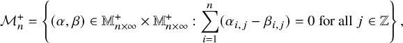 $$ \begin{align} \mathcal{M}_n^+ = \left\{ (\alpha,\beta) \in \mathbb{M}_{n \times \infty}^+ \times \mathbb{M}_{n \times \infty}^+ : \sum_{i=1}^n ( \alpha_{i,j} - \beta_{i,j} )= 0 \text{ for all } j\in \mathbb{Z} \right\}, \end{align} $$
where $\mathbb {M}_{n \times \infty }^+$
is the subspace of
$\mathbb {M}_{n \times \infty }^+$
is the subspace of $\mathbb {M}_{n \times \infty }$
of matrices
$\mathbb {M}_{n \times \infty }$
of matrices $\alpha $
such that
$\alpha $
such that $\alpha _{i,j} = 0$
if
$\alpha _{i,j} = 0$
if $j \le 0$
.
$j \le 0$
.
Proposition 2.3. The correspondence
![]() is a bijection between the set of pairs
is a bijection between the set of pairs $(P,Q)$
of classical semistandard tableaux with labels in
$(P,Q)$
of classical semistandard tableaux with labels in $\mathcal {A}_n$
and
$\mathcal {A}_n$
and $\mathcal {M}_n^+ \times \mathbb {Y}$
.
$\mathcal {M}_n^+ \times \mathbb {Y}$
.
Proof. We need to construct the inverse map $(\alpha ,\beta ;\nu ) \to (P,Q)$
. For this, define weakly increasing words
$(\alpha ,\beta ;\nu ) \to (P,Q)$
. For this, define weakly increasing words $p^{(j)},q^{(j)}$
as
$p^{(j)},q^{(j)}$
as
 $$ \begin{align} p^{(j)} = 1^{\alpha_{1,j}} 2^{\alpha_{2,j}} \cdots, \qquad q^{(j)} = 1^{\beta_{1,j}} 2^{\beta_{2,j}} \cdots. \end{align} $$
Since $(\alpha ,\beta ) \in \mathcal {M}_n^+$
,
$(\alpha ,\beta ) \in \mathcal {M}_n^+$
, $p^{(j)},q^{(j)}$
have the same length denoted by
$p^{(j)},q^{(j)}$
have the same length denoted by $\theta _j$
. Define also partition
$\theta _j$
. Define also partition $\eta $
through relations
$\eta $
through relations
 $$ \begin{align} \eta_i-\eta_{i+1} = \theta_{j+1} - \min \left\{ \mathrm{ov}(p^{(j)}, p^{(j+1)}) , \mathrm{ov}(q^{(j)}, q^{(j+1)} ) \right\}. \end{align} $$
Then $P,Q$
are the tableaux of shape
$P,Q$
are the tableaux of shape $\lambda /\rho $
with
$\lambda /\rho $
with $\lambda = \eta + \theta + \nu $
and
$\lambda = \eta + \theta + \nu $
and $\rho = \eta + \nu $
and with j-th rows given by words
$\rho = \eta + \nu $
and with j-th rows given by words $p^{(j)},q^{(j)}$
. It is straightforward to check that maps
$p^{(j)},q^{(j)}$
. It is straightforward to check that maps $(P,Q)\mapsto (\alpha ,\beta ;\nu )$
and
$(P,Q)\mapsto (\alpha ,\beta ;\nu )$
and $(\alpha ,\beta ;\nu ) \mapsto (P,Q)$
are mutual inverses.
$(\alpha ,\beta ;\nu ) \mapsto (P,Q)$
are mutual inverses.
Example 2.4. Consider the pair of semistandard tableaux
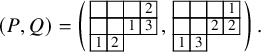
Then we have
![]() , where
, where
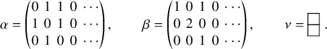
For later use, we also introduce the set
consisting on all pairs
![]() that are row-coordinate arrays of pairs of standard tableaux. At times in the text, we will also use sets
that are row-coordinate arrays of pairs of standard tableaux. At times in the text, we will also use sets $\mathcal {M}_n$
,
$\mathcal {M}_n$
, $\mathcal {Z}_n$
defined, respectively, as in equation (2.20), replacing
$\mathcal {Z}_n$
defined, respectively, as in equation (2.20), replacing $\mathbb {M}_{n\times \infty }^{+}$
by
$\mathbb {M}_{n\times \infty }^{+}$
by $\mathbb {M}_{n\times \infty }$
and equation (2.25) replacing
$\mathbb {M}_{n\times \infty }$
and equation (2.25) replacing $\mathbb {N}$
by
$\mathbb {N}$
by $\mathbb {Z}$
.
$\mathbb {Z}$
.
2.6 Standardization
We define the operation of standardization [Reference Schützenberger78] of semistandard tableaux
 $$ \begin{align} \mathrm{std} : P \in SST(\lambda / \rho , n) \mapsto P' \in ST(\lambda / \rho). \end{align} $$
Let $\gamma = (\gamma _1 ,\dots , \gamma _n)$
be the content of tableau P, and define
$\gamma = (\gamma _1 ,\dots , \gamma _n)$
be the content of tableau P, and define $\Gamma _i=\gamma _1 + \cdots + \gamma _i$
for
$\Gamma _i=\gamma _1 + \cdots + \gamma _i$
for $i=1,\dots ,n$
, where
$i=1,\dots ,n$
, where $\Gamma _0=0$
by convention. Then cells of
$\Gamma _0=0$
by convention. Then cells of $P'=\mathrm {std}(P)$
are labeled replacing i-cells of P, from the leftmost to the right with
$P'=\mathrm {std}(P)$
are labeled replacing i-cells of P, from the leftmost to the right with $\Gamma _{i-1} + 1 , \dots , \Gamma _i$
. For instance, we have
$\Gamma _{i-1} + 1 , \dots , \Gamma _i$
. For instance, we have
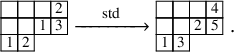
It is clear that, remembering the content $\gamma $
of the original tableaux P, one can recover P from its standardization
$\gamma $
of the original tableaux P, one can recover P from its standardization $P'$
.
$P'$
.
We present the analog of standardization in the language of matrices. Rows of matrices in $\mathbb {M}_{n\times \infty }$
are compactly supported infinite arrays of nonnegative integers, and we denote their set by
$\mathbb {M}_{n\times \infty }$
are compactly supported infinite arrays of nonnegative integers, and we denote their set by
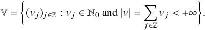 $$ \begin{align} \mathbb{V}=\bigg\{ (v_j)_{j\in \mathbb{Z}}: v_j \in \mathbb{N}_0 \text{ and } |v| = \sum_{j\in \mathbb{Z}} v_j < +\infty \bigg\}. \end{align} $$
We will write elements $v \in \mathbb {V}$
via the expansion
$v \in \mathbb {V}$
via the expansion $v= \sum _{k \in \mathbb {Z}} v_k \mathbb {e}_k $
, where
$v= \sum _{k \in \mathbb {Z}} v_k \mathbb {e}_k $
, where $\mathbb {e}_k$
is the standard basis of the infinite-dimensional vector space
$\mathbb {e}_k$
is the standard basis of the infinite-dimensional vector space $\bigoplus _{k\in \mathbb {Z}} \mathbb {C}$
. Introducing the Weyl chamber
$\bigoplus _{k\in \mathbb {Z}} \mathbb {C}$
. Introducing the Weyl chamber
we define the natural correspondence $\mathbb {W}^k \leftrightarrow \{ v \in \mathbb {V} : |v| = k\},$
by the invertible mapping
$\mathbb {W}^k \leftrightarrow \{ v \in \mathbb {V} : |v| = k\},$
by the invertible mapping
Given $\alpha \in \mathbb {M}_{n \times \infty }$
and denoting its rows by
$\alpha \in \mathbb {M}_{n \times \infty }$
and denoting its rows by $\alpha _1,\alpha _2 ,\dots $
, we define the standardization
$\alpha _1,\alpha _2 ,\dots $
, we define the standardization
![]() as the array
as the array
obtained joining smaller arrays
![]() such that
such that
![]() , under correspondence (2.30). One can check that standardization of matrices is compatible with the row-coordinate parameterization, or in other words
, under correspondence (2.30). One can check that standardization of matrices is compatible with the row-coordinate parameterization, or in other words
 $$ \begin{align} \mathrm{rc} \circ \mathrm{std} (P) = \mathrm{std} \circ \mathrm{rc} (P) \end{align} $$
for all semistandard tableaux P. An example of such commutation relation can be observed considering the semistandard tableau P on the left-hand side of equation (2.27), whose row-coordinate matrix $\alpha =\mathrm {rc}(P)$
was reported in Proposition 2.4. Then we see that both
$\alpha =\mathrm {rc}(P)$
was reported in Proposition 2.4. Then we see that both $\mathrm {std}(\alpha )$
and
$\mathrm {std}(\alpha )$
and $\mathrm {rc}(\mathrm {std}(P))$
give as a result the array
$\mathrm {rc}(\mathrm {std}(P))$
give as a result the array
![]() .
.
3 Skew
$\mathbf {RSK}$
map and edge local rules

We revisit a combinatorial operation introduced by Sagan and Stanley in [Reference Sagan and Stanley73]. In order to fully describe its properties, we will present different formulations of this construction.
3.1 Skew
$\mathbf {RSK}$
map of tableaux

In this subsection, we define the skew $\mathbf {RSK}$
map as the result of consecutive operations on pairs of tableaux
$\mathbf {RSK}$
map as the result of consecutive operations on pairs of tableaux $P,Q$
. In case
$P,Q$
. In case $P,Q$
share the same shape, this is equivalent to the definition
$P,Q$
share the same shape, this is equivalent to the definition $\mathbf {RSK}=\iota _2^n$
given in the introduction, as proven in Proposition 3.6 below.
$\mathbf {RSK}=\iota _2^n$
given in the introduction, as proven in Proposition 3.6 below.
Let P be a semistandard tableau of generalized shape $\lambda / \rho $
. A cell
$\lambda / \rho $
. A cell $(c,r) \in \lambda /\rho $
is a corner cell if
$(c,r) \in \lambda /\rho $
is a corner cell if $(c-1,r),(c,r-1) \notin \lambda /\rho $
. Consider an integer r such that P has a corner cell
$(c-1,r),(c,r-1) \notin \lambda /\rho $
. Consider an integer r such that P has a corner cell $(c,r)$
at row r. The internal insertion
$(c,r)$
at row r. The internal insertion $\mathcal {R}_{[r]}$
, first introduced in [Reference Sagan and Stanley73], is the operation that constructs tableau
$\mathcal {R}_{[r]}$
, first introduced in [Reference Sagan and Stanley73], is the operation that constructs tableau $P'=\mathcal {R}_{[r]}(P)$
vacating cell
$P'=\mathcal {R}_{[r]}(P)$
vacating cell $(c,r)$
of P and inserting value
$(c,r)$
of P and inserting value $P(c,r)$
at row
$P(c,r)$
at row $r+1$
following Schensted’s bumping algorithm. For this, we first find
$r+1$
following Schensted’s bumping algorithm. For this, we first find $\overline {c} = \min \{k : P(k,r+1)> P(c,r) \}$
. If
$\overline {c} = \min \{k : P(k,r+1)> P(c,r) \}$
. If $\overline {c}$
does not exist, we simply add a
$\overline {c}$
does not exist, we simply add a $P(c,r)$
-cell at the right of row
$P(c,r)$
-cell at the right of row $r+1$
of P. Alternatively, if
$r+1$
of P. Alternatively, if $\overline {c}$
exists, we assign cell
$\overline {c}$
exists, we assign cell $(\overline {c},r+1)$
label
$(\overline {c},r+1)$
label $P(c,r)$
and we insert, following the same mechanism,
$P(c,r)$
and we insert, following the same mechanism, $P(\overline {c},r+1)$
at row
$P(\overline {c},r+1)$
at row $r+2$
. Eventually, this algorithm stops, and the result is the tableau
$r+2$
. Eventually, this algorithm stops, and the result is the tableau $P'$
. It could also happen that we try the internal insertion
$P'$
. It could also happen that we try the internal insertion $\mathcal {R}_{[r]}$
at some row r with only empty cells. In that case, the result is tableaux with an extra empty cell at row r.
$\mathcal {R}_{[r]}$
at some row r with only empty cells. In that case, the result is tableaux with an extra empty cell at row r.
The definition of the skew $\mathbf {RSK}$
map of tableaux is given below.
$\mathbf {RSK}$
map of tableaux is given below.
Definition 3.1 (Skew
$\mathbf {RSK}$
map of tableaux).

Let $P \in SST(\lambda / \rho ,n)$
,
$P \in SST(\lambda / \rho ,n)$
, $Q \in SST(\mu / \rho ,m)$
, for some generalized Young diagrams
$Q \in SST(\mu / \rho ,m)$
, for some generalized Young diagrams $\lambda ,\mu ,\rho $
. Define the skew
$\lambda ,\mu ,\rho $
. Define the skew $\mathbf {RSK}$
map of
$\mathbf {RSK}$
map of $P,Q$
$P,Q$
 $$ \begin{align} \mathbf{RSK}(P,Q) = (P',Q') \in \bigcup_{\varkappa} SST(\varkappa / \mu,n) \times SST(\varkappa / \lambda , m) \end{align} $$
via the following algorithm. Set $P^{(0)} = P$
and
$P^{(0)} = P$
and $Q^{(0)} = \lambda /\lambda $
, that is,
$Q^{(0)} = \lambda /\lambda $
, that is, $Q^{(0)}$
has empty shape and external shape equal to
$Q^{(0)}$
has empty shape and external shape equal to $\lambda $
. For
$\lambda $
. For $j=1,\dots ,m$
, let
$j=1,\dots ,m$
, let $r^{(j)}_1\ge \cdots \ge r^{(j)}_{k_j}$
be the row coordinates of all j-cells of Q and define
$r^{(j)}_1\ge \cdots \ge r^{(j)}_{k_j}$
be the row coordinates of all j-cells of Q and define
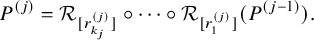 $$ \begin{align} P^{(j)} = \mathcal{R}_{[r^{(j)}_{k_j}]} \circ \cdots \circ \mathcal{R}_{[r^{(j)}_{1}]} (P^{(j-1)}). \end{align} $$
Then define $Q^{(j)}$
, adding to
$Q^{(j)}$
, adding to $Q^{(j-1)} \ j$
-cells so that the external shape of
$Q^{(j-1)} \ j$
-cells so that the external shape of $Q^{(j)}$
matches that of
$Q^{(j)}$
matches that of $P^{(j)}$
. Finally, set
$P^{(j)}$
. Finally, set $P' = P^{(m)}$
and
$P' = P^{(m)}$
and $Q'=Q^{(m)}$
. Sometimes, we will consider the skew
$Q'=Q^{(m)}$
. Sometimes, we will consider the skew $\mathbf {RSK}$
map between standard tableaux
$\mathbf {RSK}$
map between standard tableaux $(P,Q)$
, and in such case, we may call this operation skew
$(P,Q)$
, and in such case, we may call this operation skew $\mathbf {RS}$
map.
$\mathbf {RS}$
map.
The reader can check the definition of the skew $\mathbf {RSK}$
map of tableaux with the following example, where for simplicity we have taken
$\mathbf {RSK}$
map of tableaux with the following example, where for simplicity we have taken $P,Q$
of equal shape
$P,Q$
of equal shape
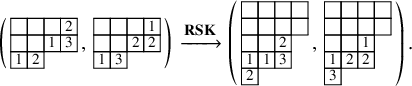
We also report step-by-step calculations
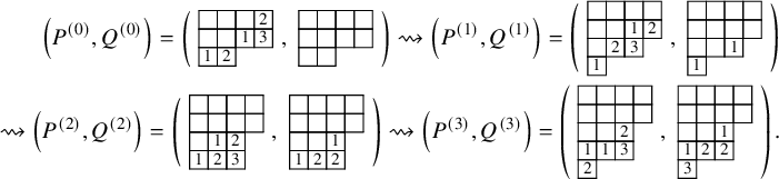
Additional examples are given in Figure 6, right panel, and in Section 1.2.
Remark 3.2. The skew $\mathbf {RSK}$
map is essentially the same as the skew Knuth map in [Reference Sagan and Stanley73], with one difference. In [Reference Sagan and Stanley73], the authors allowed the ‘external’ insertion of new cells, prescribed by a biword
$\mathbf {RSK}$
map is essentially the same as the skew Knuth map in [Reference Sagan and Stanley73], with one difference. In [Reference Sagan and Stanley73], the authors allowed the ‘external’ insertion of new cells, prescribed by a biword $\pi $
, in the original pair of classical tableaux
$\pi $
, in the original pair of classical tableaux $(P,Q)$
, so that the skew Knuth map had the form
$(P,Q)$
, so that the skew Knuth map had the form $(P,Q;\pi ) \mapsto (P',Q')$
. In our case, we don’t consider external insertions, as we imagine that cells that would be externally inserted from the biword
$(P,Q;\pi ) \mapsto (P',Q')$
. In our case, we don’t consider external insertions, as we imagine that cells that would be externally inserted from the biword $\pi $
are already present in generalized tableaux
$\pi $
are already present in generalized tableaux $(P,Q)$
, although ‘hidden’ at nonpositive rows. Therefore, external insertions in the skew Knuth map correspond, in the skew
$(P,Q)$
, although ‘hidden’ at nonpositive rows. Therefore, external insertions in the skew Knuth map correspond, in the skew $\mathbf {RSK}$
map, to cells that, following some internal insertion, move from row 0 to row 1 of the P tableau. For instance, in Figure 6, right image, we can observe that during the second step of the skew
$\mathbf {RSK}$
map, to cells that, following some internal insertion, move from row 0 to row 1 of the P tableau. For instance, in Figure 6, right image, we can observe that during the second step of the skew $\mathbf {RSK}$
map a 4-cell bumps into the first row of the P tableau, corresponding to column
$\mathbf {RSK}$
map a 4-cell bumps into the first row of the P tableau, corresponding to column $\binom {2}{4}$
of the biword denoted there by
$\binom {2}{4}$
of the biword denoted there by $\pi ^{(1)}$
.
$\pi ^{(1)}$
.
Next, we present a symmetry of the skew $\mathbf {RSK}$
map of tableaux that was proven in [Reference Sagan and Stanley73] and that will be useful in a number of cases.
$\mathbf {RSK}$
map of tableaux that was proven in [Reference Sagan and Stanley73] and that will be useful in a number of cases.
Proposition 3.3 ([Reference Sagan and Stanley73], Theorem 3.3).
If $\mathbf {RSK}(P,Q) = (P',Q')$
, then
$\mathbf {RSK}(P,Q) = (P',Q')$
, then $\mathbf {RSK}(Q,P) = (Q',P')$
.
$\mathbf {RSK}(Q,P) = (Q',P')$
.
Proposition 3.3 says that, like $P'$
and P, also the recording tableau
$P'$
and P, also the recording tableau $Q'$
is obtained from Q following a number of internal insertion. This fact is not obvious from Proposition 3.1.
$Q'$
is obtained from Q following a number of internal insertion. This fact is not obvious from Proposition 3.1.
The operation of standardization defined at the end of Section 2.2 is well behaved with respect to the skew $\mathbf {RSK}$
map, as stated in the next proposition. This was already observed in [Reference Sagan and Stanley73] and such natural reduction simplifies proofs of many statements.
$\mathbf {RSK}$
map, as stated in the next proposition. This was already observed in [Reference Sagan and Stanley73] and such natural reduction simplifies proofs of many statements.
Proposition 3.4. We have $\mathrm {std} \circ \mathbf {RSK} (P,Q) = \mathbf {RS} \circ \mathrm {std} (P,Q)$
.
$\mathrm {std} \circ \mathbf {RSK} (P,Q) = \mathbf {RS} \circ \mathrm {std} (P,Q)$
.


3.2 Operations
$\iota _1,\iota _2$
: internal insertion with cycling

Here, we introduce two operations $\iota _1,\iota _2$
on pairs of tableaux sharing the same shape. They are the same as in the introduction.
$\iota _1,\iota _2$
on pairs of tableaux sharing the same shape. They are the same as in the introduction.
Definition 3.5 (Internal insertion with cycling).
Let $(P,Q)$
be a pair of semistandard tableaux with same shape. Let
$(P,Q)$
be a pair of semistandard tableaux with same shape. Let $r_1\ge \cdots \ge r_k$
be the row coordinates of all
$r_1\ge \cdots \ge r_k$
be the row coordinates of all $1$
-cells of Q. Define
$1$
-cells of Q. Define
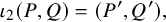 $$ \begin{align} \iota_2(P,Q) = (P', Q'), \end{align} $$
where $P' = \mathcal {R}_{[r_k]} \cdots \mathcal {R}_{[r_1]}(P)$
and
$P' = \mathcal {R}_{[r_k]} \cdots \mathcal {R}_{[r_1]}(P)$
and $Q'$
is obtained from Q vacating first all
$Q'$
is obtained from Q vacating first all $1$
-cells, subtracting 1 from the remaining entries and finally adding n-cells so that the final shape equals that of
$1$
-cells, subtracting 1 from the remaining entries and finally adding n-cells so that the final shape equals that of $P'$
. For an example, see equation (1.5). We also define
$P'$
. For an example, see equation (1.5). We also define $\iota _1=\mathrm {swap} \circ \iota _2 \circ \mathrm {swap}$
, where
$\iota _1=\mathrm {swap} \circ \iota _2 \circ \mathrm {swap}$
, where $\mathrm {swap}(x,y)=(y,x)$
.
$\mathrm {swap}(x,y)=(y,x)$
.
The next proposition states that both $\iota _1$
and
$\iota _1$
and $\iota _2$
represent refinements of the skew
$\iota _2$
represent refinements of the skew $\mathbf {RSK}$
map and that the definition of the skew
$\mathbf {RSK}$
map and that the definition of the skew $\mathbf {RSK}$
map of tableaux given in Proposition 3.1 is consistent with the one given in Section 1.2, under the assumption that
$\mathbf {RSK}$
map of tableaux given in Proposition 3.1 is consistent with the one given in Section 1.2, under the assumption that $P,Q$
have same shape.
$P,Q$
have same shape.
Proposition 3.6. For $P,Q\in SST(\lambda / \rho ,n)$
, we have
$P,Q\in SST(\lambda / \rho ,n)$
, we have
 $$ \begin{align} \iota_1^n(P,Q) = \mathbf{RSK}(P,Q) = \iota_2^n (P,Q). \end{align} $$
Proof. Denote $(\tilde {P}^{(j)},\tilde {Q}^{(j)}) = \iota _2^j(P,Q)$
for
$(\tilde {P}^{(j)},\tilde {Q}^{(j)}) = \iota _2^j(P,Q)$
for $1\leq j\leq n$
. Comparing Proposition 3.1 and Proposition 3.5, it is easy to see that
$1\leq j\leq n$
. Comparing Proposition 3.1 and Proposition 3.5, it is easy to see that $P^{(j)} = \tilde {P}^{(j)}$
and that, for all
$P^{(j)} = \tilde {P}^{(j)}$
and that, for all $k=1,\dots ,j$
, k-cells of
$k=1,\dots ,j$
, k-cells of $Q^{(j)}$
correspond to
$Q^{(j)}$
correspond to $(k+n-j)$
-cells in
$(k+n-j)$
-cells in $\tilde {Q}^{(j)}$
. Taking
$\tilde {Q}^{(j)}$
. Taking $j=n$
proves
$j=n$
proves $\iota _2^n = \mathbf {RSK}$
. The complementary statement
$\iota _2^n = \mathbf {RSK}$
. The complementary statement $\iota _1^n = \mathbf {RSK}$
follows now from the swap symmetry of Proposition 3.3.
$\iota _1^n = \mathbf {RSK}$
follows now from the swap symmetry of Proposition 3.3.
Proposition 3.7. Let $P,Q\in SST(\lambda /\rho ,n)$
. Recalling the content
$P,Q\in SST(\lambda /\rho ,n)$
. Recalling the content $\gamma $
, define
$\gamma $
, define $N_{\epsilon } = \gamma _1(P)$
if
$N_{\epsilon } = \gamma _1(P)$
if $\epsilon =1$
or
$\epsilon =1$
or $N_{\epsilon } = \gamma _1(Q)$
if
$N_{\epsilon } = \gamma _1(Q)$
if $\epsilon =2$
. Then
$\epsilon =2$
. Then $\mathrm {std} \circ \iota _{\epsilon } (P,Q) = \iota _{\epsilon }^{N_{\epsilon }} \circ \mathrm {std} (P,Q)$
.
$\mathrm {std} \circ \iota _{\epsilon } (P,Q) = \iota _{\epsilon }^{N_{\epsilon }} \circ \mathrm {std} (P,Q)$
.
Proof. This follows from the sequential definition of $\iota _1,\iota _2$
given in Proposition 3.5.
$\iota _1,\iota _2$
given in Proposition 3.5.
Proposition 3.8. Let $P,Q\in SST(\lambda /\rho ,n)$
for some
$P,Q\in SST(\lambda /\rho ,n)$
for some $\lambda ,\rho \in \mathbb {Y}$
and define
$\lambda ,\rho \in \mathbb {Y}$
and define $(\tilde {P},\tilde {Q})=\iota _{\epsilon }(P,Q)$
for
$(\tilde {P},\tilde {Q})=\iota _{\epsilon }(P,Q)$
for $\epsilon $
being either
$\epsilon $
being either $1$
or
$1$
or $2$
. Then
$2$
. Then $\ker (P,Q)=\ker (\tilde {P},\tilde {Q})$
.
$\ker (P,Q)=\ker (\tilde {P},\tilde {Q})$
.
Proof. We will only prove our claim for pairs of standard tableaux $P,Q$
and for
$P,Q$
and for $\epsilon =2$
. This implies the more general case with pairs of semistandard tableaux by Proposition 3.7. On the other hand, the case
$\epsilon =2$
. This implies the more general case with pairs of semistandard tableaux by Proposition 3.7. On the other hand, the case $\epsilon =1$
follows by the
$\epsilon =1$
follows by the $\epsilon =2$
case since the kernel of a pair of tableaux is invariant under swap, that is,
$\epsilon =2$
case since the kernel of a pair of tableaux is invariant under swap, that is, $\ker (P,Q)=\ker (Q,P)$
.
$\ker (P,Q)=\ker (Q,P)$
.
The proof presented below consists in a case-by-case analysis of the insertion procedure, and although rather technical, it is not conceptually involved. We will analyze the internal insertion of a cell in the P tableaux, and we will follow modifications that such insertion imply, showing that, in all cases, the result, paired with the corresponding changes in the Q tableau does not modify the quantity $\ker (P,Q)$
.
$\ker (P,Q)$
.
For any j, let $p^{(j)}, q^{(j)}, \tilde {p}^{(j)}, \tilde {q}^{(j)}$
be weakly increasing words recording, respectively, the j-th rows of
$p^{(j)}, q^{(j)}, \tilde {p}^{(j)}, \tilde {q}^{(j)}$
be weakly increasing words recording, respectively, the j-th rows of $P, Q, \tilde {P}, \tilde {Q}$
. Assume that the
$P, Q, \tilde {P}, \tilde {Q}$
. Assume that the $1$
-cell of Q lies at row r and that the n-cell of
$1$
-cell of Q lies at row r and that the n-cell of $\tilde {Q}$
lies at row
$\tilde {Q}$
lies at row $\bar {r}$
, that is,
$\bar {r}$
, that is, $1\in p^{(r)}$
and
$1\in p^{(r)}$
and $n\in \tilde {p}^{(\bar {r})}$
. Then we have
$n\in \tilde {p}^{(\bar {r})}$
. Then we have $\tilde {P}=\mathcal {R}_{[r]}(P)$
, and during the internal insertion a new cell gets created at row
$\tilde {P}=\mathcal {R}_{[r]}(P)$
, and during the internal insertion a new cell gets created at row $\bar {r}$
. Let
$\bar {r}$
. Let $\nu =\ker (P,Q)$
and
$\nu =\ker (P,Q)$
and $\tilde {\nu } = \ker (\tilde {P},\tilde {Q})$
. We aim to show that for each
$\tilde {\nu } = \ker (\tilde {P},\tilde {Q})$
. We aim to show that for each $j \ge 1$
we have
$j \ge 1$
we have $\nu _j - \nu _{j+1} = \tilde {\nu }_j - \tilde {\nu }_{j+1}$
. For this, we use the explicit expression of the kernel of a pair of tableaux discussed in Section 2.4, and we have
$\nu _j - \nu _{j+1} = \tilde {\nu }_j - \tilde {\nu }_{j+1}$
. For this, we use the explicit expression of the kernel of a pair of tableaux discussed in Section 2.4, and we have
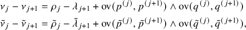 $$ \begin{align} \begin{aligned} \nu_j-\nu_{j+1} &= \rho_j - \lambda_{j+1} + \mathrm{ov}(p^{(j)},p^{(j+1)}) \wedge \mathrm{ov}(q^{(j)},q^{(j+1)}) \\ \tilde{\nu}_j-\tilde{\nu}_{j+1} &= \tilde{\rho}_j - \tilde{\lambda}_{j+1} + \mathrm{ov}(\tilde{p}^{(j)},\tilde{p}^{(j+1)}) \wedge \mathrm{ov}(\tilde{q}^{(j)},\tilde{q}^{(j+1)}), \end{aligned} \end{align} $$
where $\tilde {\lambda } / \tilde {\rho }$
is the the shape of
$\tilde {\lambda } / \tilde {\rho }$
is the the shape of $\tilde {P}, \tilde {Q}$
. Since
$\tilde {P}, \tilde {Q}$
. Since
 $$ \begin{align} \tilde{\rho}_j = \rho_j + \delta_{j,r} \qquad \text{and} \qquad \tilde{\lambda}_j = \lambda_j + \delta_{j,\bar{r}}, \end{align} $$
to prove our proposition we need to show that
 $$ \begin{align} \mathrm{ov}(\tilde{p}^{(j)},\tilde{p}^{(j+1)}) \wedge \mathrm{ov}(\tilde{q}^{(j)},\tilde{q}^{(j+1)} ) = \mathrm{ov}(p^{(j)},p^{(j+1)}) \wedge \mathrm{ov}(q^{(j)},q^{(j+1)}) - \delta_{j,r} + \delta_{j,\bar{r}-1}. \end{align} $$
We start by comparing overlaps between rows of Q and $\tilde {Q}$
. We find that
$\tilde {Q}$
. We find that
 $$ \begin{align} \mathrm{ov}(\tilde{q}^{(j)},\tilde{q}^{(j+1)}) = \mathrm{ov}(q^{(j)},q^{(j+1)}) - \mathbf{1}_{1\in q^{(j)}} + \mathbf{1}_{n \in \tilde{q}^{(j+1)}}, \end{align} $$
which follows from a simple inspection of cycling of letters in the Q tableau, and we only need to take care of rows where a cell is vacated or created. The comparison between $\mathrm {ov}(p^{(j)}, p^{(j+1)})$
and
$\mathrm {ov}(p^{(j)}, p^{(j+1)})$
and $\mathrm {ov}(\tilde {p}^{(j)}, \tilde {p}^{(j+1)})$
is more laborious, and we need to check for all different choices of j. To simplify our notation, we set
$\mathrm {ov}(\tilde {p}^{(j)}, \tilde {p}^{(j+1)})$
is more laborious, and we need to check for all different choices of j. To simplify our notation, we set $a=p^{(j)}$
,
$a=p^{(j)}$
, $b=p^{(j+1)}$
,
$b=p^{(j+1)}$
, $\tilde {a}=\tilde {p}^{(j)}$
,
$\tilde {a}=\tilde {p}^{(j)}$
, $\tilde {b}=\tilde {p}^{(j+1)}$
. If
$\tilde {b}=\tilde {p}^{(j+1)}$
. If $L=\mathrm {ov}(a,b)$
, then
$L=\mathrm {ov}(a,b)$
, then $a_i<b_{\ell (b) - L +i}$
for all
$a_i<b_{\ell (b) - L +i}$
for all $i=1,\dots ,L$
and there exists x such that
$i=1,\dots ,L$
and there exists x such that $a_x> b_{\ell (b) - L +x-1}$
. Assume that x is the smallest of such indices, and call
$a_x> b_{\ell (b) - L +x-1}$
. Assume that x is the smallest of such indices, and call $y=\ell (b) - L +x-1$
, as in Figure 4. We call
$y=\ell (b) - L +x-1$
, as in Figure 4. We call $(x,y)$
a blocking pair of depth L. It is clear that the existence of a blocking pair of depth L is equivalent to saying that
$(x,y)$
a blocking pair of depth L. It is clear that the existence of a blocking pair of depth L is equivalent to saying that $\mathrm {ov}(a,b)=L$
. Notice that such notation also covers extremal cases when
$\mathrm {ov}(a,b)=L$
. Notice that such notation also covers extremal cases when $L=\ell (a)$
, and
$L=\ell (a)$
, and $L=\ell (b)$
where we set, respectively,
$L=\ell (b)$
where we set, respectively, $x=\ell (a)+1$
and
$x=\ell (a)+1$
and $y=0$
. Let us now confirm equation (3.9) for all cases.
$y=0$
. Let us now confirm equation (3.9) for all cases.
Notation used in the proof of Proposition 3.8. Here, $L=\mathrm {ov}(a,b)$
and
$L=\mathrm {ov}(a,b)$
and $a_x>b_y$
so that x and y form a blocking pair of depth L.
$a_x>b_y$
so that x and y form a blocking pair of depth L.
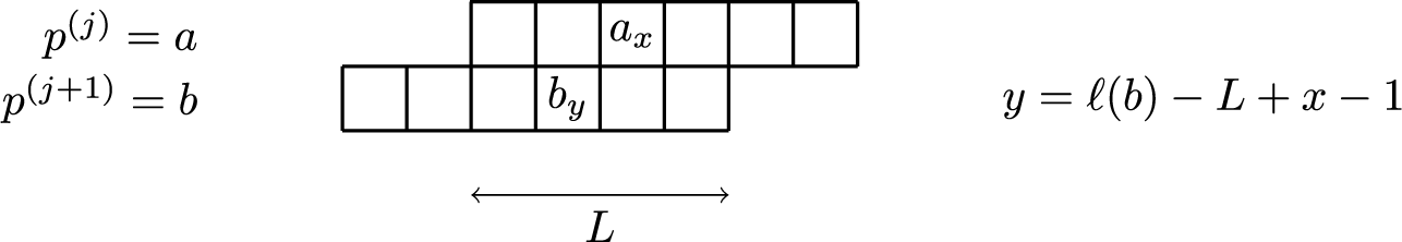
-
$j<r-1$
. In this case,
$a=\tilde {a}, b=\tilde {b}$
and by equations (3.10), (3.9) holds.
-
$j=r-1$
. Here, we have
$\tilde {a}=a$
and
$\tilde {b}=b_2 \cdots b_{\ell (b)}$
. We set
$\tilde {x}=x$
and
$\tilde {y} = y-1$
, and this is a blocking pair of depth L for
$\tilde {a},\tilde {b}$
, whenever
$y \neq 0$
. If on the other hand
$y=0$
, we have
$L=\ell (b)$
and since
$1 \in q^{(r)}$
, then
$L>\mathrm {ov}(q^{(r-1)},q^{(r)}) = \mathrm {ov}(\tilde {q}^{(r-1)},\tilde {q}^{(r)})$
, by equation (3.10). In both cases, equation (3.9) holds.
-
$j=r$
. In this case,
$\tilde {a}=a_2 \dots a_{\ell (a)}$
and
$\tilde {b}=b_1 \cdots b_{\bar {k}} \, a_1 \, b_{\bar {k}+2} \cdots b_{\ell (b)}$
for an index
$\bar {k} \in \{0,\dots ,\ell (b)\}$
. If
$\bar {k}=\ell (b)$
, then
$\mathrm {ov}(\tilde {a},\tilde {b})=L=0$
and by equation (3.10), equation (3.9) holds. Assume now that
$\bar {k}<\ell (b)$
. If
$x=1$
, then necessarily
$\bar {k} = y$
and
$\tilde {x}=1$
,
$\tilde {y}=y+1$
is a blocking pair of depth
$L-1$
for
$\tilde {a},\tilde {b}$
. If on the other hand
$x\neq 1$
, then
$\bar {k} \le y$
, and in such case we set
$\tilde {x}=x-1, \tilde {y}=y$
, which again is a blocking pair of depth
$L-1$
for
$\tilde {a},\tilde {b}$
. Overall, we have shown that
$\mathrm {ov}(\tilde {a},\tilde {b}) = \mathrm {ov}(a,b) -1 +\delta _{\bar {k} , \ell (b)}$
, which confirms equation (3.9).
-
$r<j<\bar {r}-1$
. We have
$\tilde {a}=a_1 \cdots a_{\bar {m}-1} \, z \, a_{\bar {m}+1} \cdots a_{\ell (a)}$
for some letter z and some index
$\bar {m}$
. Similarly, we have
$\tilde {b}=b_1 \cdots b_{\bar {k}} \, a_{\bar {m}} \, b_{\bar {k}+2} \cdots b_{\ell (b)}$
for an index
$\bar {k} \in \{0,\dots ,\ell (b)\}$
. If
$\bar {m}>x$
, then
$\bar {k} \ge y$
and we set
$\tilde {x}=x,\tilde {y}=y$
. If
$\bar {m}=x$
, then
$\bar {k}=y$
and we set
$\tilde {x}=x+1,\tilde {y}=y+1$
. Lastly, if
$\bar {m}<x$
necessarily
$\tilde {b}_y < \tilde {a}_x$
and we set
$\tilde {x}=x,\tilde {y}=y$
. In all cases,
$\tilde {x},\tilde {y}$
form a blocking pair of depth L for
$\tilde {a},\tilde {b}$
, confirming equation (3.9).
-
$r<j=\bar {r}-1$
. Observe that the case
$r=j=\bar {r}-1$
was already treated above. We have
$\tilde {a}=a_1 \cdots a_{\bar {m}-1} \, z \, a_{\bar {m}+1} \cdots a_{\ell (a)}$
for some letter z and some index
$\bar {m}$
and
$\tilde {b}=b_1\cdots b_{\ell (b)} \, a_{\bar {m}}$
. Since
$a_{\bar {m}}>b_k$
for all k, we necessarily have
$\bar {m}>L$
and
$\tilde {x}=x,\tilde {y}=y$
becomes a blocking pair of depth
$L+1$
for
$\tilde {a},\tilde {b}$
. Hence, from equation (3.10), (3.9) holds.
-
$j=\bar {r}$
. In this case,
$\tilde {a}=a_1\cdots a_{\ell (a)} z$
for some letter z greater than all entries of a and
$\tilde {b}=b$
. If
$\ell (a)<L$
then necessarily
$\mathrm {ov}(\tilde {a},\tilde {b}) = \mathrm {ov}(a,b)$
, which implies equation (3.10). If on the other hand
$\ell (a) = L$
, then it could happen that
$\mathrm {ov}(\tilde {a},\tilde {b}) =L+1$
, if entries of a are small and
$z<b_{\ell (b)}$
. Nevertheless, since (3.11)we always have
$$ \begin{align} \ell(a) = \ell(q^{(\bar{r})}) \ge \mathrm{ov}(q^{(\bar{r})}, q^{(\bar{r}+1)}) = \mathrm{ov}( \tilde{q}^{(\bar{r})}, \tilde{q}^{(\bar{r}+1)}), \end{align} $$
$\mathrm {ov} (\tilde {q}^{(\bar {r})}, \tilde {q}^{(\bar {r}+1)}) \le L$
and equation (3.9) holds.
-
$j>\bar {r}$
. Here,
$\tilde {a}=a$
and
$\tilde {b}= b$
so that equation (3.9) trivially holds.


The previous list of checks exhausts all the cases and completes the proof.
3.3 The skew RS map of arrays
In this subsection, we introduce the skew $\mathbf {RS}$
map of pairs of arrays, following [Reference Viennot89]. Due to the correspondence between arrays and standard tableaux, it provides a diagrammatic realization of the skew
$\mathbf {RS}$
map of pairs of arrays, following [Reference Viennot89]. Due to the correspondence between arrays and standard tableaux, it provides a diagrammatic realization of the skew $\mathbf {RS}$
map for standard tableaux, as will be seen in Proposition 3.14. It represents a reformulation of the shadow line construction by Viennot [Reference Viennot88], as we see now.
$\mathbf {RS}$
map for standard tableaux, as will be seen in Proposition 3.14. It represents a reformulation of the shadow line construction by Viennot [Reference Viennot88], as we see now.
Definition 3.9 (Shadow line construction).
Let
![]() be a pair of arrays and
be a pair of arrays and $\Lambda _{m,n}=\{1,\dots , m\} \times \{ 1,\dots , n\}$
be a finite rectangular lattice. From the left edge of each cell
$\Lambda _{m,n}=\{1,\dots , m\} \times \{ 1,\dots , n\}$
be a finite rectangular lattice. From the left edge of each cell $(1,i)$
for
$(1,i)$
for $i=1,\ldots ,n$
(resp. bottom edge of each cell
$i=1,\ldots ,n$
(resp. bottom edge of each cell $(j,1)$
for
$(j,1)$
for $j=1,\ldots , m$
), start drawing a line of color
$j=1,\ldots , m$
), start drawing a line of color
![]() to the right (resp. of color
to the right (resp. of color
![]() to the top). We draw the line configuration until every cell of
to the top). We draw the line configuration until every cell of $\Lambda _{m,n}$
is crossed both vertically and horizontally, using the following rules. Lines of different colors cross each other, while if two lines of the same color C meet, then from the intersection point they will proceed in their rightward and upward run with their color upgraded to
$\Lambda _{m,n}$
is crossed both vertically and horizontally, using the following rules. Lines of different colors cross each other, while if two lines of the same color C meet, then from the intersection point they will proceed in their rightward and upward run with their color upgraded to $C+1$
. The ensemble of lines on
$C+1$
. The ensemble of lines on $\Lambda _{m,n}$
generated with this procedure is called shadow line construction.
$\Lambda _{m,n}$
generated with this procedure is called shadow line construction.
For an example of a shadow line construction, see Figure 5. There in correspondence to intersection points of lines with the same color C we drew bullets of color $C+1$
. The rules of assigning colors to lines in this construction can be translated into local rules of configurations on edges of the lattice [Reference Fomin27, Reference Viennot89].
$C+1$
. The rules of assigning colors to lines in this construction can be translated into local rules of configurations on edges of the lattice [Reference Fomin27, Reference Viennot89].
The shadow line construction for
![]() and
and
![]() , equivalent to the skew
, equivalent to the skew $\mathbf {RS}$
map in the left panel of Figure 6
$\mathbf {RS}$
map in the left panel of Figure 6
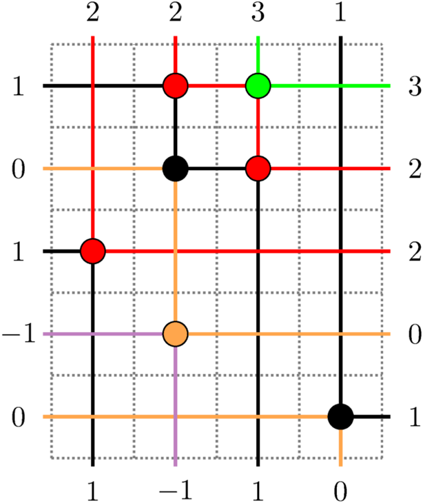
In the left panel, we see the graphical representation of the skew $\mathbf {RS}$
map
$\mathbf {RS}$
map
![]() between
between
![]() ,
,
![]() . We have colored each edge of the grid based on its value. Black bullets denote faces where north and east edges take simultaneously value 1 defining partial permutation
. We have colored each edge of the grid based on its value. Black bullets denote faces where north and east edges take simultaneously value 1 defining partial permutation $\pi^{(1)}=\left( \begin{smallmatrix} 2 & 4 \\ 4 & 1 \end{smallmatrix} \right) $
. In the right panel, we reported on the left and bottom sides the tableaux
$\pi^{(1)}=\left( \begin{smallmatrix} 2 & 4 \\ 4 & 1 \end{smallmatrix} \right) $
. In the right panel, we reported on the left and bottom sides the tableaux $(P,Q)$
and on the right and top sides tableaux
$(P,Q)$
and on the right and top sides tableaux $(P',Q') = \mathbf {RS}(P,Q)$
. One can check that
$(P',Q') = \mathbf {RS}(P,Q)$
. One can check that
![]() and
and
![]() .
.
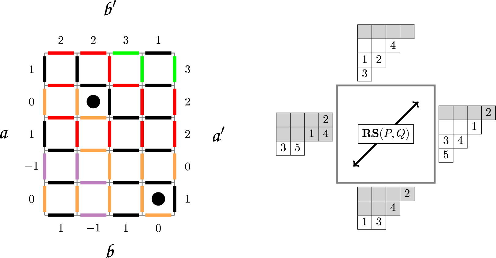
Definition 3.10 (
$\mathbb {Z}$
-valued edge configurations).

On a planar lattice $\Lambda \subseteq \mathbb {Z}\times \mathbb {Z}$
,
$\Lambda \subseteq \mathbb {Z}\times \mathbb {Z}$
, $\mathbb {Z}$
-valued edge configurations
$\mathbb {Z}$
-valued edge configurations $\mathcal {E}$
are quadruples of functions
$\mathcal {E}$
are quadruples of functions $(\mathsf {W},\mathsf {S},\mathsf {E},\mathsf {N}):\Lambda \to \mathbb {Z}$
such that
$(\mathsf {W},\mathsf {S},\mathsf {E},\mathsf {N}):\Lambda \to \mathbb {Z}$
such that $\mathsf {E}(c) = \mathsf {W}(c+\mathbf {e}_1)$
and
$\mathsf {E}(c) = \mathsf {W}(c+\mathbf {e}_1)$
and $\mathsf {N}(c) = \mathsf {S}(c+\mathbf {e}_2)$
for all points
$\mathsf {N}(c) = \mathsf {S}(c+\mathbf {e}_2)$
for all points $c\in \Lambda $
where these conditions make sense. We say that
$c\in \Lambda $
where these conditions make sense. We say that $\mathcal {E}$
is admissible if it satisfies the local rules
$\mathcal {E}$
is admissible if it satisfies the local rules
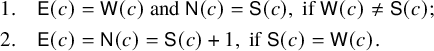 $$ \begin{align} &1.\quad \mathsf{E}(c) = \mathsf{W}(c) \text{ and } \mathsf{N}(c) = \mathsf{S}(c), \text{ if } \mathsf{W}(c) \ne \mathsf{S}(c);\\&2.\quad \mathsf{E}(c) = \mathsf{N}(c) = \mathsf{S}(c)+1, \text{ if } \mathsf{S}(c)=\mathsf{W}(c).\nonumber \end{align} $$
In this language, we define the skew $\mathbf {RS}$
map of arrays as follows.
$\mathbf {RS}$
map of arrays as follows.
Definition 3.11 (Skew
$\mathbf {RS}$
map of arrays).

Let
![]() be a pair of arrays. Consider the unique admissible edge configuration on
be a pair of arrays. Consider the unique admissible edge configuration on $\Lambda _{m,n}$
with
$\Lambda _{m,n}$
with
![]() ,
,
![]() for all
for all $i=1,\dots ,n$
,
$i=1,\dots ,n$
, $j=1,\dots ,m$
. The skew
$j=1,\dots ,m$
. The skew $\mathbf {RS}$
map of
$\mathbf {RS}$
map of
![]() is the pair
is the pair
![]() given by
given by
![]() and
and
![]() for
for $i=1,\dots ,n$
,
$i=1,\dots ,n$
, $j=1,\dots ,m$
.
$j=1,\dots ,m$
.
For an example of edge configurations and an evaluation of the skew $\mathbf {RS}$
map of two arrays, corresponding to Figure 5, see Figure 6, left panel. Note that positions
$\mathbf {RS}$
map of two arrays, corresponding to Figure 5, see Figure 6, left panel. Note that positions $(j,i)$
of bullets of color k are determined by the condition
$(j,i)$
of bullets of color k are determined by the condition $\mathsf {N}(j,i) = \mathsf {E}(j,i) =k$
. We will encode the positions
$\mathsf {N}(j,i) = \mathsf {E}(j,i) =k$
. We will encode the positions $(j_1,i_1),(j_2,i_2),\dots $
of bullets of color k in the partial permutation
$(j_1,i_1),(j_2,i_2),\dots $
of bullets of color k in the partial permutation
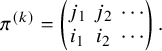 $$ \begin{align} \pi^{(k)} = \left( \begin{matrix} j_1 & j_2 & \cdots \\ i_1 & i_2 & \cdots \end{matrix} \right). \end{align} $$
Using edge configurations, we also define operators of $\iota _1,\iota _2$
on pairs of arrays.
$\iota _1,\iota _2$
on pairs of arrays.
Definition 3.12 (
$\iota _1,\iota _2$
on arrays).

Let
![]() be a pair of arrays that are permutations of each other, and consider on
be a pair of arrays that are permutations of each other, and consider on $\Lambda _{n,n}$
the unique admissible edge configuration with
$\Lambda _{n,n}$
the unique admissible edge configuration with
![]() for all
for all $i=1,\dots ,n$
. Define
$i=1,\dots ,n$
. Define
![]() setting
setting

Analogously, define
![]() .
.
Comparing 3.11 and 3.12, we see that $\mathbf {RS}=\iota _1^n=\iota _2^n$
holds as operations on pairs of arrays.
$\mathbf {RS}=\iota _1^n=\iota _2^n$
holds as operations on pairs of arrays.
The next proposition shows that $\iota _1,\iota _2$
, both as operations on pairs of standard tableaux and on pairs of arrays, coincide, modulo row-coordinate parameterization.
$\iota _1,\iota _2$
, both as operations on pairs of standard tableaux and on pairs of arrays, coincide, modulo row-coordinate parameterization.
Proposition 3.13. Let $P,Q \in ST(\lambda /\rho )$
and
$P,Q \in ST(\lambda /\rho )$
and
![]() . Then
. Then
![]() , for both
, for both $\epsilon =1,2$
.
$\epsilon =1,2$
.
Proof. We prove our statement only for the case $\epsilon =2$
, as the remaining case is analogous. The fact that
$\epsilon =2$
, as the remaining case is analogous. The fact that $\nu =\ker (P,Q)$
does not change after the application of
$\nu =\ker (P,Q)$
does not change after the application of $\iota _2$
was shown in Proposition 3.8. Therefore, we need to show that if
$\iota _2$
was shown in Proposition 3.8. Therefore, we need to show that if $(\tilde {P},\tilde {Q})=\iota _2(P,Q)$
and
$(\tilde {P},\tilde {Q})=\iota _2(P,Q)$
and
![]() , we have
, we have
![]() .
.
Call
, so that $\tilde {P}=\mathcal {R}_{[r]}(P)$
. Suppose that during the internal insertion bumping happens k times and cells of P at location
$\tilde {P}=\mathcal {R}_{[r]}(P)$
. Suppose that during the internal insertion bumping happens k times and cells of P at location $(c_j,r+j)$
move to
$(c_j,r+j)$
move to $(c_{j+1},r+j+1)$
for
$(c_{j+1},r+j+1)$
for $j=0,\dots ,k-1$
. Denoting
$j=0,\dots ,k-1$
. Denoting $p_j=P(c_j,r+j)$
, we have
$p_j=P(c_j,r+j)$
, we have $c_0 \ge c_1 \ge \cdots \ge c_k$
and
$c_0 \ge c_1 \ge \cdots \ge c_k$
and $p_0 < p_1 < \cdots < p_{k-1}$
. In the row-coordinate array
$p_0 < p_1 < \cdots < p_{k-1}$
. In the row-coordinate array
, this implies that
and importantly
for $\ell =1,\dots , p_{j+1} - p_j$
. We also have
$\ell =1,\dots , p_{j+1} - p_j$
. We also have
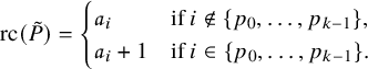
On the other hand, we now draw the edge configuration on $\Lambda _{n,n}$
corresponding to the pair
$\Lambda _{n,n}$
corresponding to the pair
as for equation (3.12) and we see that $S(1,i)=W(1,i)=r+j,p_j\leq i<p_{j+1},0\leq j\leq k-1$
and
$S(1,i)=W(1,i)=r+j,p_j\leq i<p_{j+1},0\leq j\leq k-1$
and $E(1,i)=N(1,i)=r+j+1$
. Comparing this with the definition of
$E(1,i)=N(1,i)=r+j+1$
. Comparing this with the definition of $\iota _2$
in equation (3.14), we can confirm that
$\iota _2$
in equation (3.14), we can confirm that
holds.
To show that
![]() notice that, from the cycling of labels, the i-cell of
notice that, from the cycling of labels, the i-cell of $\tilde {Q}$
lies at row
$\tilde {Q}$
lies at row
![]() for
for $i=1,\dots ,n-1$
. On the other hand, the n-cell of
$i=1,\dots ,n-1$
. On the other hand, the n-cell of $\tilde {Q}$
lies at row
$\tilde {Q}$
lies at row $r+k$
, which, by the computation above is also the value of
$r+k$
, which, by the computation above is also the value of
![]() . This completes the proof.
. This completes the proof.
The coincidence extends to the skew $\mathbf {RS}$
maps.
$\mathbf {RS}$
maps.
Corollary 3.14. Let $P,Q \in ST(\lambda /\rho )$
and
$P,Q \in ST(\lambda /\rho )$
and
![]() . Then
. Then
![]() .
.
Proof. This follows from Proposition 3.13 and from the fact that $\mathbf {RS}=\iota _{\epsilon }^n$
, with
$\mathbf {RS}=\iota _{\epsilon }^n$
, with $n=|\lambda / \rho |$
and
$n=|\lambda / \rho |$
and $\epsilon =1,2$
, both as operations on pairs of arrays or on pairs of tableaux.
$\epsilon =1,2$
, both as operations on pairs of arrays or on pairs of tableaux.
Corollary 3.15. Let $P,Q \in ST(\lambda /\rho )$
and
$P,Q \in ST(\lambda /\rho )$
and
![]() . Consider the admissible edge configuration on
. Consider the admissible edge configuration on $\Lambda _{n,n}$
corresponding to the pair
$\Lambda _{n,n}$
corresponding to the pair
![]() as in Proposition 3.11. Fix
as in Proposition 3.11. Fix $i,j\in \{1,\dots ,n\}$
and
$i,j\in \{1,\dots ,n\}$
and $k\in \mathbb {Z}$
. Then,
$k\in \mathbb {Z}$
. Then, $\mathsf {N}(j,i)=\mathsf {E}(j,i) = k$
if and only if during the evaluation of the skew
$\mathsf {N}(j,i)=\mathsf {E}(j,i) = k$
if and only if during the evaluation of the skew $\mathbf {RS}$
map
$\mathbf {RS}$
map $(P,Q) \to (P',Q')$
, at the step corresponding to internal insertions of j-cells of Q, the i-cell of the P-tableau moves from row
$(P,Q) \to (P',Q')$
, at the step corresponding to internal insertions of j-cells of Q, the i-cell of the P-tableau moves from row $k-1$
to row k.
$k-1$
to row k.
Proof. For $j=1$
and
$j=1$
and $i\in \{1,\dots ,n\}$
, this follows from the computations reported in the Proposition 3.13. Iterating the operations
$i\in \{1,\dots ,n\}$
, this follows from the computations reported in the Proposition 3.13. Iterating the operations $\iota _2$
yields the general j case.
$\iota _2$
yields the general j case.
We finally report a simple ‘restriction property’ of the shadow line construction. For the next proposition, we need the notion of partial arrays, which are elements of $(\mathbb {Z} \cup \{\varnothing \})^n$
. Given an array
$(\mathbb {Z} \cup \{\varnothing \})^n$
. Given an array
![]() , we denote by
, we denote by
![]() the partial array with entries
the partial array with entries
![]() if
if
![]() and
and
![]() otherwise.
otherwise.
Proposition 3.16. Let
![]() and
and
![]() . For a fixed k, let
. For a fixed k, let $\pi ^{(k)}$
be the partial permutation defined by equation (3.13). Then the partial arrays
$\pi ^{(k)}$
be the partial permutation defined by equation (3.13). Then the partial arrays
![]() depend uniquely on
depend uniquely on
![]() and
and $\pi ^{(k)}$
.
$\pi ^{(k)}$
.
Proof. This is immediate from the definition of the shadow line construction or equivalently from local rules (3.12). Entries of arrays
![]() correspond to shadow lines with colors greater than or equal to k. Such lines either enter the lattice from west or south and hence are given by
correspond to shadow lines with colors greater than or equal to k. Such lines either enter the lattice from west or south and hence are given by
![]() or alternatively are created within the grid, in which case are determined by the knowledge of
or alternatively are created within the grid, in which case are determined by the knowledge of $\pi ^{(k)}$
.
$\pi ^{(k)}$
.
Remark 3.17. In case
![]() , the partial permutation
, the partial permutation $\pi ^{(k)}$
determines completely
$\pi ^{(k)}$
determines completely
![]() . Setting
. Setting $k=1$
, this corresponds to the shadow line construction of the classical Robinson–Schensted correspondence [Reference Sagan74].
$k=1$
, this corresponds to the shadow line construction of the classical Robinson–Schensted correspondence [Reference Sagan74].
3.4 The skew RSK map of matrices
We extend the operation of skew $\mathbf {RS}$
map to include infinite matrices of integers. Thanks to the correspondence between matrices and tableaux of Proposition 2.3, this provides a diagrammatic realization of the skew
$\mathbf {RS}$
map to include infinite matrices of integers. Thanks to the correspondence between matrices and tableaux of Proposition 2.3, this provides a diagrammatic realization of the skew $\mathbf {RSK}$
map for tableaux. By the standardization most of their properties follow directly from the ones of the skew
$\mathbf {RSK}$
map for tableaux. By the standardization most of their properties follow directly from the ones of the skew $\mathbf {RS}$
map.
$\mathbf {RS}$
map.
We can generalize the shadow line construction of Proposition 3.9 by allowing edges of the lattice $\Lambda _{m,n}$
to be crossed by arbitrary many lines. We impose that on each cell for any two lines crossing the same horizontal (resp. vertical) edge the one with higher color stays at the left (resp. below) of the one with lower color; see Figure 7. This implies also that for each color bullets at a cell lie strictly to the right of those at cells
$\Lambda _{m,n}$
to be crossed by arbitrary many lines. We impose that on each cell for any two lines crossing the same horizontal (resp. vertical) edge the one with higher color stays at the left (resp. below) of the one with lower color; see Figure 7. This implies also that for each color bullets at a cell lie strictly to the right of those at cells $c-k \mathbf {e}_2$
and strictly above those at cells
$c-k \mathbf {e}_2$
and strictly above those at cells $c-k \mathbf {e}_1$
for all
$c-k \mathbf {e}_1$
for all $k\in \mathbb {N}_0$
. We record the list of colored lines crossing a specific edge in an array
$k\in \mathbb {N}_0$
. We record the list of colored lines crossing a specific edge in an array $v\in \mathbb {V}$
and for any
$v\in \mathbb {V}$
and for any $C\in \mathbb {Z}$
the value
$C\in \mathbb {Z}$
the value $v_C$
will count the number of C-colored lines; see Figure 8. Such discussion justifies the following definition.
$v_C$
will count the number of C-colored lines; see Figure 8. Such discussion justifies the following definition.
Generalized shadow line construction on the lattice $\Lambda _{3,3}$
.
$\Lambda _{3,3}$
.
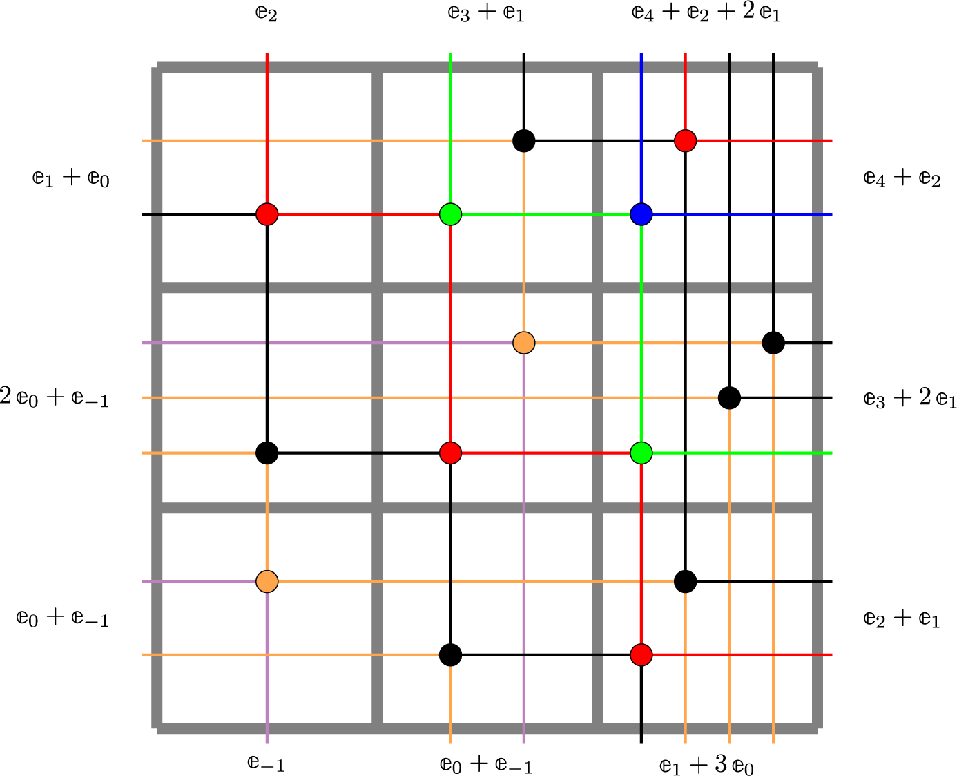
On the left panel, we see the equivalence between $\mathbb {V}$
-valued edge configurations and configurations of colored lines through a face. On the right panel, a graphical interpretation of local rules (3.16)
$\mathbb {V}$
-valued edge configurations and configurations of colored lines through a face. On the right panel, a graphical interpretation of local rules (3.16)
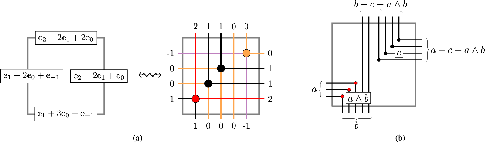
Definition 3.18 (
$\mathbb {V}$
-valued edge configurations).

For a planar lattice $\Lambda \subseteq \mathbb {Z}\times \mathbb {Z}$
, define
$\Lambda \subseteq \mathbb {Z}\times \mathbb {Z}$
, define $\mathbb {V}$
-valued edge configurations
$\mathbb {V}$
-valued edge configurations $\mathcal {E}$
as quadruples of functions
$\mathcal {E}$
as quadruples of functions $(\mathsf {W},\mathsf {S},\mathsf {E},\mathsf {N}):\Lambda \to \mathbb {V}$
such that
$(\mathsf {W},\mathsf {S},\mathsf {E},\mathsf {N}):\Lambda \to \mathbb {V}$
such that $\mathsf {E}(c)=\mathsf {W}(c+\mathbf {e}_1)$
and
$\mathsf {E}(c)=\mathsf {W}(c+\mathbf {e}_1)$
and $\mathsf {N}(c)=\mathsf {S}(c+\mathbf {e}_2)$
for all
$\mathsf {N}(c)=\mathsf {S}(c+\mathbf {e}_2)$
for all $c\in \Lambda $
. An edge configuration is admissible if it satisfies the local rules
$c\in \Lambda $
. An edge configuration is admissible if it satisfies the local rules
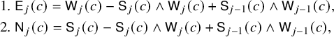 $$ \begin{align} \begin{aligned}&1. \ \mathsf{E}_j(c) = \mathsf{W}_j(c) - \mathsf{S}_j(c) \wedge \mathsf{W}_j(c) + \mathsf{S}_{j-1}(c) \wedge \mathsf{W}_{j-1}(c), \\&2. \ \mathsf{N}_j(c) = \mathsf{S}_j(c) - \mathsf{S}_j(c) \wedge \mathsf{W}_j(c) + \mathsf{S}_{j-1}(c) \wedge \mathsf{W}_{j-1}(c),\end{aligned} \end{align} $$
for all $c\in \Lambda $
,
$c\in \Lambda $
, $j\in \mathbb {Z}$
. Here
$j\in \mathbb {Z}$
. Here $a\wedge b=\min (a,b)$
.
$a\wedge b=\min (a,b)$
.
Local rules (3.16) describe the arrangement of lines of the each color j around single faces of the lattice. Namely, $\mathsf {W}_j(c)$
is the number of j-colored lines entering face c from the left and similarly for
$\mathsf {W}_j(c)$
is the number of j-colored lines entering face c from the left and similarly for $\mathsf {S}_j, \mathsf {E}_j, \mathsf {N}_j$
. We report this statement in the next proposition, and we refer to Figure 8 for the graphical interpretation of such rules.
$\mathsf {S}_j, \mathsf {E}_j, \mathsf {N}_j$
. We report this statement in the next proposition, and we refer to Figure 8 for the graphical interpretation of such rules.
Proposition 3.19. On the lattice $\Lambda _{1,1}$
, consisting of a single face, consider the admissible
$\Lambda _{1,1}$
, consisting of a single face, consider the admissible $\mathbb {V}$
-valued edge configuration
$\mathbb {V}$
-valued edge configuration $\mathsf {W}=a, \mathsf {S}=b, \mathsf {E}=a', \mathsf {N}=b'$
. Consider arrays
$\mathsf {W}=a, \mathsf {S}=b, \mathsf {E}=a', \mathsf {N}=b'$
. Consider arrays
![]() ,
,
![]() such that
such that
![]() under the map
under the map $v:\mathbb {W}^k \to \mathbb {V}$
defined in equation (2.30). Then
$v:\mathbb {W}^k \to \mathbb {V}$
defined in equation (2.30). Then
![]() .
.
Proof. This is straightforward after a comparison of local rules (3.16) with the skew $\mathbf {RS}$
map of weakly decreasing arrays
$\mathbf {RS}$
map of weakly decreasing arrays
![]() corresponding to the generic edge values
corresponding to the generic edge values $a,b$
.
$a,b$
.
In line with Section 2.6, we can define the standardization of an admissible $\mathbb {V}$
-valued edge configuration
$\mathbb {V}$
-valued edge configuration $\mathcal {E}$
on a lattice
$\mathcal {E}$
on a lattice $\Lambda $
. This will be the admissible
$\Lambda $
. This will be the admissible $\mathbb {Z}$
-valued edge configuration
$\mathbb {Z}$
-valued edge configuration $\mathcal {E}'=\mathrm {std}(\mathcal {E})$
on the lattice
$\mathcal {E}'=\mathrm {std}(\mathcal {E})$
on the lattice $\Lambda '$
obtained from
$\Lambda '$
obtained from $\mathcal {E}$
‘blowing up’ faces of
$\mathcal {E}$
‘blowing up’ faces of $\Lambda $
as prescribed by Proposition 3.19.
$\Lambda $
as prescribed by Proposition 3.19.
Definition 3.20 (Skew
$\mathbf {RSK}$
map of matrices).

Let $\alpha \in \mathbb {M}_{n\times \infty },\beta \in \mathbb {M}_{m\times \infty }$
, and consider the unique
$\alpha \in \mathbb {M}_{n\times \infty },\beta \in \mathbb {M}_{m\times \infty }$
, and consider the unique $\mathbb {V}$
-valued admissible edge configuration on
$\mathbb {V}$
-valued admissible edge configuration on $\Lambda _{m,n}$
such that
$\Lambda _{m,n}$
such that $\mathsf {W}_k(1,i)=\alpha _{i,k}$
,
$\mathsf {W}_k(1,i)=\alpha _{i,k}$
, $\mathsf {S}_k(j,1)=\beta _{j,k}$
, for all
$\mathsf {S}_k(j,1)=\beta _{j,k}$
, for all $i=1,\dots ,n$
,
$i=1,\dots ,n$
, $j=1,\dots ,m$
,
$j=1,\dots ,m$
, $k\in \mathbb {Z}$
. We define the skew
$k\in \mathbb {Z}$
. We define the skew $\mathbf {RSK}$
map
$\mathbf {RSK}$
map
 $$ \begin{align*} \mathbf{RSK}(\alpha,\beta)=(\alpha',\beta') \in \mathbb{M}_{n\times \infty} \times \mathbb{M}_{m \times \infty}, \end{align*} $$
as the pair of matrices $\alpha _{i,k}^{\prime }=\mathsf {E}_k(m,i)$
,
$\alpha _{i,k}^{\prime }=\mathsf {E}_k(m,i)$
, $\beta _{j,k}^{\prime }=\mathsf {N}_k(j,n)$
, for all
$\beta _{j,k}^{\prime }=\mathsf {N}_k(j,n)$
, for all $i=1,\dots ,n$
,
$i=1,\dots ,n$
, $j=1,\dots ,m$
,
$j=1,\dots ,m$
, $k\in \mathbb {Z}$
. From the configuration, define also the family of matrices
$k\in \mathbb {Z}$
. From the configuration, define also the family of matrices $M^{(k)}$
as
$M^{(k)}$
as
 $$ \begin{align} M^{(k)}(j,i) = \mathsf{N}_k(j,i) \wedge \mathsf{E}_k(j,i). \end{align} $$
Example 3.21. Define matrices
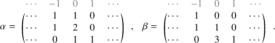
We evaluate $(\alpha ',\beta ') = \mathbf {RSK}(\alpha , \beta )$
computing the corresponding
$(\alpha ',\beta ') = \mathbf {RSK}(\alpha , \beta )$
computing the corresponding $\mathbb {V}$
-valued edge configuration on
$\mathbb {V}$
-valued edge configuration on $\Lambda _{3,3}$
. The result is reported in Figure 7, and we have
$\Lambda _{3,3}$
. The result is reported in Figure 7, and we have
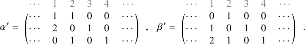
To configuration of Figure 7, we associate matrices $M^{(k)}$
as described by equation (3.17). For instance, from the same figure one can check that
$M^{(k)}$
as described by equation (3.17). For instance, from the same figure one can check that $M^{(1)}=\left ( \begin {smallmatrix} 0 & 1 & 0 \\ 1 & 0 & 2 \\ 0 & 1 & 1 \end {smallmatrix} \right )$
or
$M^{(1)}=\left ( \begin {smallmatrix} 0 & 1 & 0 \\ 1 & 0 & 2 \\ 0 & 1 & 1 \end {smallmatrix} \right )$
or $M^{(2)}=\left ( \begin {smallmatrix} 1 & 0 & 1 \\ 0 & 1 & 0 \\ 0 & 0 & 1 \end {smallmatrix} \right )$
.
$M^{(2)}=\left ( \begin {smallmatrix} 1 & 0 & 1 \\ 0 & 1 & 0 \\ 0 & 0 & 1 \end {smallmatrix} \right )$
.
Definition 3.22. For a pair of matrices $(\alpha ,\beta ) \in \mathcal {M}_n$
, construct on
$(\alpha ,\beta ) \in \mathcal {M}_n$
, construct on $\Lambda _{n,n}$
the corresponding
$\Lambda _{n,n}$
the corresponding $\mathbb {V}$
-valued edge configuration as in Proposition 3.20. We define
$\mathbb {V}$
-valued edge configuration as in Proposition 3.20. We define $\iota _2(\alpha ,\beta ) = (\tilde {\alpha }, \tilde {\beta })$
, setting for all
$\iota _2(\alpha ,\beta ) = (\tilde {\alpha }, \tilde {\beta })$
, setting for all $k\in \mathbb {Z}$
 $$ \begin{align} \tilde{\alpha}_{i,k} = \mathsf{W}_k(2,i) \qquad \text{for } i=1\dots,n \qquad \text{and} \qquad \tilde{\beta}_{i,k} = \begin{cases} \mathsf{S}_k(i+1,1) \quad &\text{if } i=1,\dots,n-1, \\ \mathsf{N}_k(1,n) \quad &\text{if } i=n. \end{cases} \end{align} $$
Operator $\iota _1$
is defined by duality
$\iota _1$
is defined by duality $\iota _1(\alpha ,\beta )=\mathrm {swap} \circ \iota _2 \circ \mathrm {swap} (\alpha ,\beta )$
.
$\iota _1(\alpha ,\beta )=\mathrm {swap} \circ \iota _2 \circ \mathrm {swap} (\alpha ,\beta )$
.
Notice that, in the previous definition, also the pair $(\tilde {\alpha },\tilde {\beta })$
belongs to the set
$(\tilde {\alpha },\tilde {\beta })$
belongs to the set $\mathcal {M}_n$
.
$\mathcal {M}_n$
.
Proposition 3.23. Let $P,Q \in SST(\lambda /\rho ,n)$
and
$P,Q \in SST(\lambda /\rho ,n)$
and
![]() . Then
. Then
![]() , for both
, for both $\epsilon =1,2$
and
$\epsilon =1,2$
and
![]() .
.
Proof. This is a consequence of the analogous statement for standard tableaux and arrays stated in Proposition 3.13 and of Proposition 3.19.
Geometric interpretation of operators $\iota _1,\iota _2$
provided by Proposition 3.23 yields a visual proof of the nontrivial fact that they commute with each other.
$\iota _1,\iota _2$
provided by Proposition 3.23 yields a visual proof of the nontrivial fact that they commute with each other.
Proposition 3.24. We have $\iota _1 \circ \iota _2 = \iota _2 \circ \iota _1$
, both as operations on pairs of tableaux or on pairs of matrices.
$\iota _1 \circ \iota _2 = \iota _2 \circ \iota _1$
, both as operations on pairs of tableaux or on pairs of matrices.
Proof. We first prove that $\iota _1$
and
$\iota _1$
and $\iota _2$
commute when they act on pairs of matrices. Consider the admissible
$\iota _2$
commute when they act on pairs of matrices. Consider the admissible $\mathbb {V}$
-valued edge configuration on the lattice
$\mathbb {V}$
-valued edge configuration on the lattice $\Lambda _{n+1,n+1}$
such that for all
$\Lambda _{n+1,n+1}$
such that for all $k\in \mathbb {Z}$
 $$ \begin{align*} \mathsf{W}_k(1,i) = \alpha_{i,k}, \qquad \mathsf{S}_k(1,i) = \beta_{i,k}, \qquad \text{for } i=1,\dots,n \\ \text{and} \qquad \mathsf{W}_k(1,n+1) = \mathsf{E}_k(n,1) \qquad \mathsf{S}_k(n+1,1) = \mathsf{N}_k(1,n). \end{align*} $$
In this lattice, $\iota _1$
and
$\iota _1$
and $\iota _2$
act, respectively, as upward and rightward shift so that defining
$\iota _2$
act, respectively, as upward and rightward shift so that defining $\tilde {\alpha }$
,
$\tilde {\alpha }$
, $\tilde {\beta }$
as
$\tilde {\beta }$
as
 $$ \begin{align} \tilde{\alpha}_{i,k} = \mathsf{W}_k(2,i+1), \qquad \tilde{\beta}_{i,k} = \mathsf{N}_k(i+1,2), \qquad \text{for } i=1,\dots,n \text{ and } k\in \mathbb{Z} \end{align} $$
we easily see that $(\tilde {\alpha } , \tilde {\beta }) = \iota _1 \circ \iota _2 (\alpha ,\beta ) = \iota _2 \circ \iota _1 (\alpha ,\beta )$
. This proves the proposition for the case of action on pairs of matrices. By Proposition 3.23, the same commutation holds when
$(\tilde {\alpha } , \tilde {\beta }) = \iota _1 \circ \iota _2 (\alpha ,\beta ) = \iota _2 \circ \iota _1 (\alpha ,\beta )$
. This proves the proposition for the case of action on pairs of matrices. By Proposition 3.23, the same commutation holds when $\iota _1,\iota _2$
act on pair of semistandard tableaux.
$\iota _1,\iota _2$
act on pair of semistandard tableaux.
Proposition 3.25. Let $P,Q \in SST(\lambda /\rho ,n)$
and
$P,Q \in SST(\lambda /\rho ,n)$
and
![]() . Consider the admissible
. Consider the admissible $\mathbb {V}$
-valued edge configuration on
$\mathbb {V}$
-valued edge configuration on $\Lambda _{n,n}$
corresponding to the pair
$\Lambda _{n,n}$
corresponding to the pair $\alpha ,\beta $
as in Proposition 3.20. Fix
$\alpha ,\beta $
as in Proposition 3.20. Fix $i,j\in \{1,\dots ,n\}$
and
$i,j\in \{1,\dots ,n\}$
and $k\in \mathbb {Z}$
. Then,
$k\in \mathbb {Z}$
. Then, $\mathsf {N}_k(j,i) \wedge \mathsf {E}_k(j,i) = m$
if and only if during the evaluation of the skew
$\mathsf {N}_k(j,i) \wedge \mathsf {E}_k(j,i) = m$
if and only if during the evaluation of the skew $\mathbf {RSK}$
map
$\mathbf {RSK}$
map $(P,Q) \to (P',Q')$
, at the step corresponding to internal insertions of j-cells of Q, exactly
$(P,Q) \to (P',Q')$
, at the step corresponding to internal insertions of j-cells of Q, exactly $m \ i$
-cells of the P-tableau move from row
$m \ i$
-cells of the P-tableau move from row $k-1$
to row k.
$k-1$
to row k.
Proof. The analogous property for standard tableaux was given in Proposition 3.15. Combining this with Proposition 3.19 yields the statement for pairs of semistandard tableaux $P,Q$
.
$P,Q$
.
The next proposition gives a restriction property analogous to Proposition 3.16. For any matrix $\alpha \in \mathbb {M}_{n,\infty }$
, we define its truncation
$\alpha \in \mathbb {M}_{n,\infty }$
, we define its truncation $\delta _{\ge k}(\alpha ) = ( \mathbf {1}_{j\ge k} \alpha _{i,j} :i=1,\dots ,n,j\in \mathbb {Z})$
.
$\delta _{\ge k}(\alpha ) = ( \mathbf {1}_{j\ge k} \alpha _{i,j} :i=1,\dots ,n,j\in \mathbb {Z})$
.
Proposition 3.26. Let $(\alpha ,\beta )\in \mathcal {M}_n$
and
$(\alpha ,\beta )\in \mathcal {M}_n$
and $(\tilde {\alpha },\tilde {\beta })=\mathbf {RSK}(\alpha ,\beta )$
. For a fixed k, let
$(\tilde {\alpha },\tilde {\beta })=\mathbf {RSK}(\alpha ,\beta )$
. For a fixed k, let $M^{(k)}$
be the partial permutation defined by equation (3.17). Then the truncated matrices
$M^{(k)}$
be the partial permutation defined by equation (3.17). Then the truncated matrices $\delta _{\ge k}(\tilde {\alpha }), \delta _{\ge k}(\tilde {\beta })$
depend uniquely on
$\delta _{\ge k}(\tilde {\alpha }), \delta _{\ge k}(\tilde {\beta })$
depend uniquely on $\delta _{\ge k}(\alpha ), \delta _{\ge k}(\beta )$
and
$\delta _{\ge k}(\alpha ), \delta _{\ge k}(\beta )$
and $M^{(k)}$
. Moreover, for all k we have
$M^{(k)}$
. Moreover, for all k we have $(\delta _{\ge k}(\tilde {\alpha }), \delta _{\ge k}(\tilde {\beta }) ) \in \mathcal {M}_n$
.
$(\delta _{\ge k}(\tilde {\alpha }), \delta _{\ge k}(\tilde {\beta }) ) \in \mathcal {M}_n$
.
4 Skew
$\mathbf {RSK}$
and Viennot dynamics

In this section, we first introduce the skew $\mathbf {RSK}$
dynamics for a pair of tableaux by iterations of the skew
$\mathbf {RSK}$
dynamics for a pair of tableaux by iterations of the skew $\mathbf {RSK}$
maps studied in the previous section. A related dynamics, this time on the set of matrices
$\mathbf {RSK}$
maps studied in the previous section. A related dynamics, this time on the set of matrices $\overline {\mathbb {M}}_{n \times n}$
, which we call the Viennot dynamics, is also defined, and it will play an important role when describing conservation laws in Section 6.
$\overline {\mathbb {M}}_{n \times n}$
, which we call the Viennot dynamics, is also defined, and it will play an important role when describing conservation laws in Section 6.
4.1 The skew
$\mathbf {RSK}$
dynamics

The following definition was sketched in the introductory chapter.
Definition 4.1 (Skew
$\mathbf {RSK}$
dynamics).

We define a deterministic dynamics on the space of pairs of generalized tableaux by iterating the skew $\mathbf {RSK}$
map. Fix
$\mathbf {RSK}$
map. Fix $P,Q\in SST(\lambda / \rho ,n)$
, and define the skew
$P,Q\in SST(\lambda / \rho ,n)$
, and define the skew $\mathbf {RSK}$
dynamics with initial data
$\mathbf {RSK}$
dynamics with initial data $(P,Q)$
as
$(P,Q)$
as
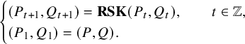 $$ \begin{align} \begin{cases} (P_{t+1},Q_{t+1})=\mathbf{RSK}(P_t,Q_t), \qquad t \in \mathbb{Z}, \\ (P_1,Q_1)=(P,Q). \end{cases} \end{align} $$
Analogously, we define the skew $\mathbf {RSK}$
dynamics on the space of pairs of matrices. For a fixed initial state
$\mathbf {RSK}$
dynamics on the space of pairs of matrices. For a fixed initial state $(\alpha ,\beta )\in \mathcal {M}_n$
, we have
$(\alpha ,\beta )\in \mathcal {M}_n$
, we have
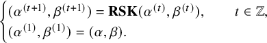 $$ \begin{align} \begin{cases} (\alpha^{(t+1)},\beta^{(t+1)})=\mathbf{RSK}(\alpha^{(t)},\beta^{(t)}), \qquad t \in \mathbb{Z}, \\ (\alpha^{(1)},\beta^{(1)})=(\alpha,\beta). \end{cases} \end{align} $$
Since the skew $\mathbf {RSK}$
map is invertible, we see that each realization of the dynamics is uniquely characterized by its initial state. This observation is very powerful as it implies that specific properties of tableaux
$\mathbf {RSK}$
map is invertible, we see that each realization of the dynamics is uniquely characterized by its initial state. This observation is very powerful as it implies that specific properties of tableaux $(P,Q)$
can be deduced observing their state at an arbitrary time of the skew
$(P,Q)$
can be deduced observing their state at an arbitrary time of the skew $\mathbf {RSK}$
dynamics. As already pointed out in Section 1.2, dynamics (4.1) presents conservation laws, that we will characterize in Section 6 and Section 9 below. Moreover, in Section 7 we will devise a linearization technique of the dynamics, which one can regard as a combinatorial variant of the inverse scattering method for classical integrable systems. The study of asymptotic states of the dynamics will be exceptionally revealing.
$\mathbf {RSK}$
dynamics. As already pointed out in Section 1.2, dynamics (4.1) presents conservation laws, that we will characterize in Section 6 and Section 9 below. Moreover, in Section 7 we will devise a linearization technique of the dynamics, which one can regard as a combinatorial variant of the inverse scattering method for classical integrable systems. The study of asymptotic states of the dynamics will be exceptionally revealing.
4.2 Edge configurations on the twisted cylinder
In the Section 3, we have seen the equivalence between the two versions of the skew $\mathbf {RSK}$
maps on tableaux and on matrices through edge local rules on a finite rectangular lattice. Here, we introduce an infinite lattice with certain periodicity and edge configurations compatible with it. This will lead us to define a dynamics on the same lattice, which is closely related to the skew
$\mathbf {RSK}$
maps on tableaux and on matrices through edge local rules on a finite rectangular lattice. Here, we introduce an infinite lattice with certain periodicity and edge configurations compatible with it. This will lead us to define a dynamics on the same lattice, which is closely related to the skew $\mathbf {RSK}$
dynamics.
$\mathbf {RSK}$
dynamics.
Definition 4.2 (Twisted cylinder).
The twisted cylinder is the periodic lattice $\mathscr {C}_n= \mathbb {Z}^2 / \sim _n$
, where
$\mathscr {C}_n= \mathbb {Z}^2 / \sim _n$
, where $(j,i)\sim _n(j', i')$
if
$(j,i)\sim _n(j', i')$
if $(j',i') = (j+kn,j-kn)$
for some
$(j',i') = (j+kn,j-kn)$
for some $k\in \mathbb {Z}$
. Natural representations of
$k\in \mathbb {Z}$
. Natural representations of $\mathscr {C}_n$
we will use are (see Figure 9):
$\mathscr {C}_n$
we will use are (see Figure 9):
 $$ \begin{align} \begin{aligned}&\kern-11pt\text{the infinite vertical strip } \{ 1, \dots , n\} \times \mathbb{Z}, \text{ where we impose faces } (n,i) \text{ and } (1,i+n) \text{ to be }\\&\kern-11pt\text{adjacent for all } j.\end{aligned} \end{align} $$
 $$ \begin{align} \begin{aligned}&\text{the infinite horizontal strip } \mathbb{Z} \times \{ 1, \dots , n\} \text{ where we impose faces } (j,n) \text{ and } (j+n,1) \text{ to be }\\&\text{adjacent for all } j.\end{aligned} \end{align} $$
Two graphical representation of the twisted cylinder $\mathscr {C}_3$
. Blue line represents an up-right path, while red line a down-right loop.
$\mathscr {C}_3$
. Blue line represents an up-right path, while red line a down-right loop.
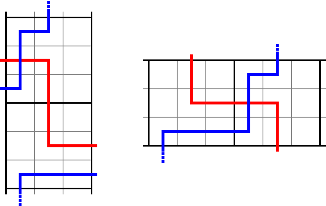
A down-right loop $\xi $
on
$\xi $
on $\mathscr {C}_n$
is a sequence
$\mathscr {C}_n$
is a sequence $(\xi _k: k\in \{1,\dots ,2n\}) \subset \mathscr {C}_n$
, such that
$(\xi _k: k\in \{1,\dots ,2n\}) \subset \mathscr {C}_n$
, such that
 $$ \begin{align} \xi_{k+1} \sim_n \xi_{k} + \mathbf{e}_1, \qquad \text{or} \qquad \xi_{k+1} \sim_n \xi_{k} - \mathbf{e}_2, \end{align} $$
for $k=1,\dots , 2n$
, where indices are taken
$k=1,\dots , 2n$
, where indices are taken $\mod 2n$
. An example of a down-right loop is the red path drawn in Figure 9, having the form
$\mod 2n$
. An example of a down-right loop is the red path drawn in Figure 9, having the form
 $$ \begin{align*}c \to c+\mathbf{e}_1 \to \cdots \to c+n\mathbf{e}_1 \to c+n\mathbf{e}_1-\mathbf{e}_2 \to \cdots \to c+n\mathbf{e}_1-(n-1)\mathbf{e}_2 \to c \end{align*} $$
for some $c\in \mathscr {C}_n$
. Assigning edge values along a down-right loop
$c\in \mathscr {C}_n$
. Assigning edge values along a down-right loop $\xi $
automatically determines the full configuration
$\xi $
automatically determines the full configuration $\mathcal {E}$
on
$\mathcal {E}$
on $\mathscr {C}_n$
as a result of local rules (3.16). We use this to visualize the skew
$\mathscr {C}_n$
as a result of local rules (3.16). We use this to visualize the skew $\mathbf {RSK}$
dynamics on the set of matrices as an edge configuration on
$\mathbf {RSK}$
dynamics on the set of matrices as an edge configuration on $\mathscr {C}_n$
. To any pair
$\mathscr {C}_n$
. To any pair $(\alpha , \beta ) \in \mathcal {M}_n$
we associate the edge configuration
$(\alpha , \beta ) \in \mathcal {M}_n$
we associate the edge configuration $\mathcal {E}$
on
$\mathcal {E}$
on $\mathscr {C}_n$
identified by the assignment
$\mathscr {C}_n$
identified by the assignment
 $$ \begin{align} (\alpha , \beta) \mapsto \mathcal{E} \qquad \colon \qquad \mathsf{E}_k(n, i) = \alpha_{i,k}, \qquad \mathsf{N}_k (i,n) = \beta_{i,k}, \qquad \text{for } i=1,\dots,n, \,\,k\in \mathbb{Z}. \end{align} $$
The subclass of admissible edge configurations accessible through mapping (4.6) is defined next.
Definition 4.3. Let $\mathcal {E}$
be a
$\mathcal {E}$
be a $\mathbb {V}$
-valued admissible edge configurations on
$\mathbb {V}$
-valued admissible edge configurations on $\mathscr {C}_n$
and for any fixed
$\mathscr {C}_n$
and for any fixed $c\in \mathscr {C}_n$
define the pair
$c\in \mathscr {C}_n$
define the pair $(\alpha , \beta )_c$
as
$(\alpha , \beta )_c$
as $\alpha _{i,k} = \mathsf {W}_k(c+ (i-1) \mathbf {e}_2)$
and
$\alpha _{i,k} = \mathsf {W}_k(c+ (i-1) \mathbf {e}_2)$
and $\beta _{i,k} = \mathsf {S}_k(c+ (i-1) \mathbf {e}_1)$
for
$\beta _{i,k} = \mathsf {S}_k(c+ (i-1) \mathbf {e}_1)$
for $i=1,\dots ,n$
,
$i=1,\dots ,n$
, $k\in \mathbb {Z}$
. We define the set
$k\in \mathbb {Z}$
. We define the set $\mathfrak {E}_n$
consisting of all configurations
$\mathfrak {E}_n$
consisting of all configurations $\mathcal {E}$
such that
$\mathcal {E}$
such that $(\alpha ,\beta )_c \in \mathcal {M}_n$
for all
$(\alpha ,\beta )_c \in \mathcal {M}_n$
for all $c\in \mathscr {C}_n$
.
$c\in \mathscr {C}_n$
.
Proposition 4.4. The sets $\mathcal {M}_n$
and
$\mathcal {M}_n$
and $\mathfrak {E}_n$
are in bijection.
$\mathfrak {E}_n$
are in bijection.
Proof. We only need to show that configuration $\mathcal {E}$
defined by equation (4.6) belongs to
$\mathcal {E}$
defined by equation (4.6) belongs to $\mathfrak {E}_n$
. Notice first that, in the notation of Proposition 4.3 we have
$\mathfrak {E}_n$
. Notice first that, in the notation of Proposition 4.3 we have $(\alpha ,\beta ) = (\alpha ,\beta )_{(1,n+1)}$
. For fixed
$(\alpha ,\beta ) = (\alpha ,\beta )_{(1,n+1)}$
. For fixed $N_1,N_2 \in \mathbb {Z}$
, let
$N_1,N_2 \in \mathbb {Z}$
, let $(\widetilde {\alpha },\widetilde {\beta })=\iota _1^{N_1} \circ \iota _2^{N_2} (\alpha ,\beta )$
. Then, by Proposition 3.22 and taking into account periodicity of
$(\widetilde {\alpha },\widetilde {\beta })=\iota _1^{N_1} \circ \iota _2^{N_2} (\alpha ,\beta )$
. Then, by Proposition 3.22 and taking into account periodicity of $\mathscr {C}_n$
we have
$\mathscr {C}_n$
we have $(\tilde {\alpha },\tilde {\beta })=(\alpha ,\beta )_{(1+N_2, n+N_1+1)}$
. Since
$(\tilde {\alpha },\tilde {\beta })=(\alpha ,\beta )_{(1+N_2, n+N_1+1)}$
. Since $(\tilde {\alpha },\tilde {\beta }) \in \mathcal {M}_n$
for all
$(\tilde {\alpha },\tilde {\beta }) \in \mathcal {M}_n$
for all $N_1,N_2$
, by Proposition 3.23, then
$N_1,N_2$
, by Proposition 3.23, then $\mathcal {E} \in \mathfrak {E}_n$
.
$\mathcal {E} \in \mathfrak {E}_n$
.
Proposition 4.5. Let $(\alpha ^{(t)},\beta ^{(t)})$
be the skew
$(\alpha ^{(t)},\beta ^{(t)})$
be the skew $\mathbf {RSK}$
dynamics with initial data
$\mathbf {RSK}$
dynamics with initial data $(\alpha ^{(1)},\beta ^{(1)}) =(\alpha ,\beta ) \in \mathcal {M}_n$
, and let
$(\alpha ^{(1)},\beta ^{(1)}) =(\alpha ,\beta ) \in \mathcal {M}_n$
, and let $\mathcal {E}$
be the configuration associated to
$\mathcal {E}$
be the configuration associated to $(\alpha ,\beta )$
by equation (4.6). Then, for all
$(\alpha ,\beta )$
by equation (4.6). Then, for all $i=1,\dots ,n$
and
$i=1,\dots ,n$
and $t \in \mathbb {Z}$
we have
$t \in \mathbb {Z}$
we have $(\alpha ^{(t)},\beta ^{(t)}) = (\alpha ,\beta )_{(1,tn+1)}$
; see Figure 10.
$(\alpha ^{(t)},\beta ^{(t)}) = (\alpha ,\beta )_{(1,tn+1)}$
; see Figure 10.
A visualization of the skew $\mathbf {RSK}$
dynamics of matrices
$\mathbf {RSK}$
dynamics of matrices $(\alpha ^{(t)},\beta ^{(t)})$
as edges of a configuration
$(\alpha ^{(t)},\beta ^{(t)})$
as edges of a configuration $\mathcal {E}$
. Faces of
$\mathcal {E}$
. Faces of $\mathscr {C}_n$
have coordinates
$\mathscr {C}_n$
have coordinates $(j,i-kn)$
.
$(j,i-kn)$
.
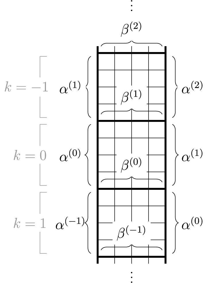
In the left panel, we see the evaluation of Viennot map transforming $\overline {\pi }$
of equation (4.9). This is done through the periodic shadow line construction explained in Proposition 4.6 and represented in the right panel. We made cells of
$\overline {\pi }$
of equation (4.9). This is done through the periodic shadow line construction explained in Proposition 4.6 and represented in the right panel. We made cells of $\mathscr {C}_n$
fatter in order to allocate multiple bullets while letting them keep the correct relative positions.
$\mathscr {C}_n$
fatter in order to allocate multiple bullets while letting them keep the correct relative positions.
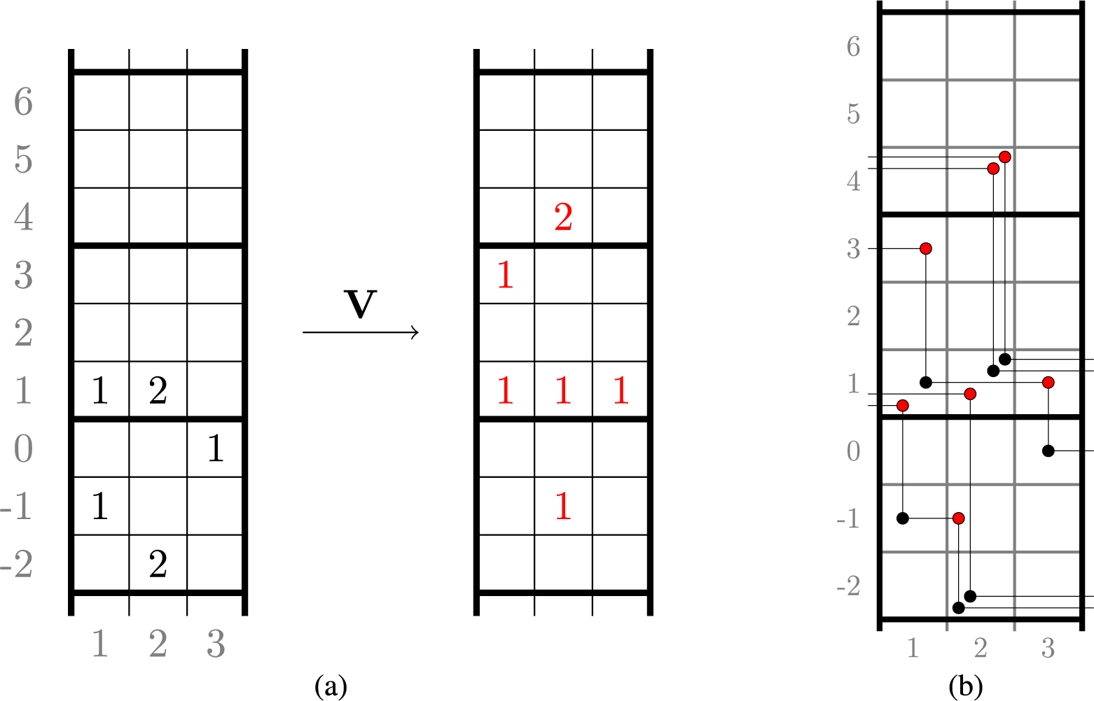
4.3 Periodic shadow line construction and Viennot dynamics
Edge configurations $\mathcal {E} \in \mathfrak {E}_n$
, in analogy with the finite case, identify families of compactly supported maps
$\mathcal {E} \in \mathfrak {E}_n$
, in analogy with the finite case, identify families of compactly supported maps $\overline {M}^{(t)}:\mathscr {C}_n \to \mathbb {N}_0$
assigning
$\overline {M}^{(t)}:\mathscr {C}_n \to \mathbb {N}_0$
assigning
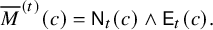 $$ \begin{align} \overline{M}^{(t)}(c) = \mathsf{N}_t(c) \wedge \mathsf{E}_t(c). \end{align} $$
On the other hand, as proven in Proposition 4.9 below, for any map $\overline {M} \in \overline {\mathbb {M}}_{n\times n}$
we can construct the family
$\overline {M} \in \overline {\mathbb {M}}_{n\times n}$
we can construct the family $\overline {M}^{(t)}$
, with the convention that
$\overline {M}^{(t)}$
, with the convention that $\overline {M}^{(1)}=\overline {M}$
and the configuration
$\overline {M}^{(1)}=\overline {M}$
and the configuration $\mathcal {E}$
such that equation (4.7) holds. Such procedure constitutes a periodic variant of the Viennot shadow line construction [Reference Viennot88] or of Fulton’s matrix ball construction [Reference Fulton31].
$\mathcal {E}$
such that equation (4.7) holds. Such procedure constitutes a periodic variant of the Viennot shadow line construction [Reference Viennot88] or of Fulton’s matrix ball construction [Reference Fulton31].
Definition 4.6 (Viennot map).
Let $\overline {M}\in \overline {\mathbb {M}}_{n\times n}$
. At each face
$\overline {M}\in \overline {\mathbb {M}}_{n\times n}$
. At each face $c \in \mathscr {C}_n$
, allocate
$c \in \mathscr {C}_n$
, allocate $\overline {M}(c)$
black bullets and apply the shadow line construction explained at the beginning of Section 3.4, letting each bullet emanate two black rays in the north and east directions. By periodicity of
$\overline {M}(c)$
black bullets and apply the shadow line construction explained at the beginning of Section 3.4, letting each bullet emanate two black rays in the north and east directions. By periodicity of $\mathscr {C}_n$
and the fact that there are only a finite number of black bullets, each ray terminates somewhere intersecting with another. The collection of such mutual intersections of rays determines a new generation of red bullets (see Figure 11, right panel), and we define
$\mathscr {C}_n$
and the fact that there are only a finite number of black bullets, each ray terminates somewhere intersecting with another. The collection of such mutual intersections of rays determines a new generation of red bullets (see Figure 11, right panel), and we define
 $$ \begin{align} \overline{M}'(c) = \# \text{ of new generation bullets at cell } c. \end{align} $$
The map $\mathbf {V} :\overline {M} \mapsto \overline {M}'$
takes the name of Viennot map. Using correspondence (2.6), we define the action of Viennot map also on weighted biwords
$\mathbf {V} :\overline {M} \mapsto \overline {M}'$
takes the name of Viennot map. Using correspondence (2.6), we define the action of Viennot map also on weighted biwords $\mathbf {V}(\overline {\pi }) = \overline {\pi }'$
, imposing
$\mathbf {V}(\overline {\pi }) = \overline {\pi }'$
, imposing $\overline {M}(\overline {\pi }')= \mathbf {V}(\overline {M}(\overline {\pi }))$
.
$\overline {M}(\overline {\pi }')= \mathbf {V}(\overline {M}(\overline {\pi }))$
.
An example of evaluation of map $\mathbf {V}$
is reported in Figure 11(a). There, we see the transition
$\mathbf {V}$
is reported in Figure 11(a). There, we see the transition
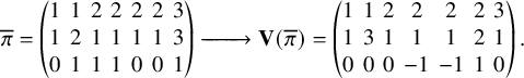 $$ \begin{align} \overline{\pi} = \left( \begin{matrix} 1 & 1 & 2 & 2 & 2 & 2 & 3 \\ 1 & 2 & 1 & 1 & 1 & 1 & 3 \\ 0 & 1 & 1 & 1 & 0 & 0 & 1 \end{matrix} \right) \xrightarrow[]{\hspace{.6cm}} \mathbf{V}(\overline{\pi}) = \left( \begin{matrix} 1 & 1 & 2 & 2 & 2 & 2 & 3 \\ 1 & 3 & 1 & 1 & 1 & 2 & 1 \\ 0 & 0 & 0 & -1 & -1 & 1 & 0 \end{matrix} \right). \end{align} $$
The shadow lines produced by the computation of $\overline {\pi } \mapsto \mathbf {V}(\overline {\pi })$
consist in a sequence of connected broken lines as we see in Figure 11(b). Recording the cells of
$\overline {\pi } \mapsto \mathbf {V}(\overline {\pi })$
consist in a sequence of connected broken lines as we see in Figure 11(b). Recording the cells of $\mathscr {C}_n$
visited by each of these broken lines, we naturally define a sequence of down-right loops
$\mathscr {C}_n$
visited by each of these broken lines, we naturally define a sequence of down-right loops $\xi ^{(1)},\xi ^{(2)},\dots $
. We will use these loops later in Section 6. For instance, in Figure 11 (b), the two topmost loops have the same form
$\xi ^{(1)},\xi ^{(2)},\dots $
. We will use these loops later in Section 6. For instance, in Figure 11 (b), the two topmost loops have the same form
 $$ \begin{align} (1,4) \to (2,4) \to (2,3) \to (2,2) \to (2,1) \to (3,1) \to (1,4). \end{align} $$
The map $\mathbf {V}$
can be thought as a generator of a deterministic dynamics on the space
$\mathbf {V}$
can be thought as a generator of a deterministic dynamics on the space $\overline {\mathbb {M}}_{n\times n}$
.
$\overline {\mathbb {M}}_{n\times n}$
.
Definition 4.7 (Viennot dynamics).
Fix $\overline {M} \in \overline {\mathbb {M}}_{n\times n}$
, and define the Viennot dynamics with initial data
$\overline {M} \in \overline {\mathbb {M}}_{n\times n}$
, and define the Viennot dynamics with initial data $\overline {M}$
as
$\overline {M}$
as
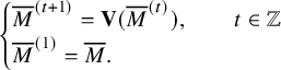 $$ \begin{align} \begin{cases} \overline{M}^{(t+1)} = \mathbf{V}(\overline{M}^{(t)}),\qquad t\in \mathbb{Z} \\ \overline{M}^{(1)} = \overline{M}. \end{cases} \end{align} $$
Analogously, for $\overline {\pi }\in \overline {\mathbb {A}}_{n,n}$
, one defines the Viennot dynamics
$\overline {\pi }\in \overline {\mathbb {A}}_{n,n}$
, one defines the Viennot dynamics $\overline {\pi }^{(t+1)}=\mathbf {V}(\overline {\pi }^{(t)})$
with initial data
$\overline {\pi }^{(t+1)}=\mathbf {V}(\overline {\pi }^{(t)})$
with initial data $\overline {\pi }^{(1)}=\overline {\pi }$
.
$\overline {\pi }^{(1)}=\overline {\pi }$
.
Remark 4.8. This may be considered a generalization of shadow line construction on $\Lambda _{n,n}$
of classical RS correspondence; see Remark 3.17.
$\Lambda _{n,n}$
of classical RS correspondence; see Remark 3.17.
Proposition 4.9. The sets $\mathfrak {E}_n$
,
$\mathfrak {E}_n$
, $\mathcal {M}_n$
and
$\mathcal {M}_n$
and $\overline {\mathbb {M}}_{n \times n}$
are in bijection
$\overline {\mathbb {M}}_{n \times n}$
are in bijection
Proof. The bijection between $\mathfrak {E}_n$
and
$\mathfrak {E}_n$
and $\mathcal {M}_n$
is proven in Proposition 4.4. We then need to prove that the assignment
$\mathcal {M}_n$
is proven in Proposition 4.4. We then need to prove that the assignment
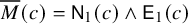 $$ \begin{align} \overline{M}(c) = \mathsf{N}_1(c) \wedge \mathsf{E}_1(c) \end{align} $$
defines a bijection $\overline {M} \mapsto \mathcal {E}$
between
$\overline {M} \mapsto \mathcal {E}$
between $\overline {\mathbb {M}}_{n \times n}$
and
$\overline {\mathbb {M}}_{n \times n}$
and $\mathfrak {E}_n$
. Let
$\mathfrak {E}_n$
. Let $\overline {M}^{(t)}$
be the Viennot dynamics with initial data
$\overline {M}^{(t)}$
be the Viennot dynamics with initial data $\overline {M}$
. Then for any
$\overline {M}$
. Then for any $c\in \mathscr {C}_n$
we set
$c\in \mathscr {C}_n$
we set $\mathsf {W}_t(c)$
as the number of lines of the construction
$\mathsf {W}_t(c)$
as the number of lines of the construction $\overline {M}^{(t)} \to \overline {M}^{(t+1)}$
entering the face c from west and similarly for
$\overline {M}^{(t)} \to \overline {M}^{(t+1)}$
entering the face c from west and similarly for $\mathsf {S}_t,\mathsf {E}_t,\mathsf {N}_t$
. From such edge configuration, define
$\mathsf {S}_t,\mathsf {E}_t,\mathsf {N}_t$
. From such edge configuration, define $(\alpha ^{(t)},\beta ^{(t)}) = (\alpha ,\beta )_{(1,tn+1)}$
, following the notation of Proposition 4.3 and recall the truncation operator
$(\alpha ^{(t)},\beta ^{(t)}) = (\alpha ,\beta )_{(1,tn+1)}$
, following the notation of Proposition 4.3 and recall the truncation operator $\delta _{\ge 1}$
from Proposition 3.26. Since
$\delta _{\ge 1}$
from Proposition 3.26. Since $\overline {M}$
is compactly supported there exists
$\overline {M}$
is compactly supported there exists $k^*> 0$
such that
$k^*> 0$
such that $\overline {M}_{i,j}(k)=0$
for all
$\overline {M}_{i,j}(k)=0$
for all $i,j\in \{1,\dots ,n\}$
and
$i,j\in \{1,\dots ,n\}$
and $|k|>k^*$
. This implies that
$|k|>k^*$
. This implies that $\delta _{\ge 1}(\alpha ^{(-k^*)}) = \delta _{\ge 1}(\beta ^{(-k^*)}) = 0$
and
$\delta _{\ge 1}(\alpha ^{(-k^*)}) = \delta _{\ge 1}(\beta ^{(-k^*)}) = 0$
and $\delta _{\ge 1}(\alpha ^{(k^*)}) = \alpha ^{(k^*)}$
,
$\delta _{\ge 1}(\alpha ^{(k^*)}) = \alpha ^{(k^*)}$
, $\delta _{\ge 1}(\beta ^{(k^*)}) = \beta ^{(k*)}$
. By recursive application of Proposition 3.26, we find that
$\delta _{\ge 1}(\beta ^{(k^*)}) = \beta ^{(k*)}$
. By recursive application of Proposition 3.26, we find that $(\alpha ^{(k^*)},\beta ^{(k^*)}) \in \mathcal {M}_n$
and they are uniquely determined. This implies that
$(\alpha ^{(k^*)},\beta ^{(k^*)}) \in \mathcal {M}_n$
and they are uniquely determined. This implies that $\mathcal {E}\in \mathfrak {E}_n$
completing the proof. Now that we have constructed the correspondence
$\mathcal {E}\in \mathfrak {E}_n$
completing the proof. Now that we have constructed the correspondence $\overline {M} \leftrightarrow \mathcal {E}$
, we can associate to the matrix
$\overline {M} \leftrightarrow \mathcal {E}$
, we can associate to the matrix $\overline {M}$
the pair
$\overline {M}$
the pair $(\alpha ,\beta )$
as in equation (4.6).
$(\alpha ,\beta )$
as in equation (4.6).
Remark 4.10. The notation $\overline {M}^{(t)}$
appeared already in equation (4.7) before Proposition 4.7, but they are consistent because, if a matrix
$\overline {M}^{(t)}$
appeared already in equation (4.7) before Proposition 4.7, but they are consistent because, if a matrix $\overline {M}$
and a configuration
$\overline {M}$
and a configuration $\mathcal {E}$
are in correspondence and
$\mathcal {E}$
are in correspondence and $\overline {M}^{(t)}$
is the Viennot dynamics with initial data
$\overline {M}^{(t)}$
is the Viennot dynamics with initial data $\overline {M}$
, then equation (4.7) holds.
$\overline {M}$
, then equation (4.7) holds.
If a pair $(\alpha ,\beta ) \in \mathcal {M}_n$
and a matrix
$(\alpha ,\beta ) \in \mathcal {M}_n$
and a matrix $\overline {M} \in \overline {\mathbb {M}}_{n \times n}$
are in correspondence through the bijection described in Proposition 4.9, we will use the notation
$\overline {M} \in \overline {\mathbb {M}}_{n \times n}$
are in correspondence through the bijection described in Proposition 4.9, we will use the notation
![]() . Moreover, composing such correspondence with the row-coordinate parameterization
. Moreover, composing such correspondence with the row-coordinate parameterization $(P,Q) \xrightarrow []{} (\alpha ,\beta )$
defines a projection denoted by
$(P,Q) \xrightarrow []{} (\alpha ,\beta )$
defines a projection denoted by
 $$ \begin{align} (P,Q) \xrightarrow[]{\mathbf{SS} \,} \overline{M}. \end{align} $$
An analogous projection $(P,Q) \xrightarrow []{\mathbf {SS} \,} \overline {\pi } \in \overline {\mathbb {A}}_{n,n}$
is defined taking advantage of mapping (2.6).
$(P,Q) \xrightarrow []{\mathbf {SS} \,} \overline {\pi } \in \overline {\mathbb {A}}_{n,n}$
is defined taking advantage of mapping (2.6).
By the same arguments as in proof of Proposition 4.9, $\mathcal {M}_n^+$
and
$\mathcal {M}_n^+$
and $\overline {\mathbb {M}}_{n \times n}^+$
are also in bijection. Combining this with the bijection between
$\overline {\mathbb {M}}_{n \times n}^+$
are also in bijection. Combining this with the bijection between $\mathcal {M}_n^+\times \mathbb {Y}$
and pairs
$\mathcal {M}_n^+\times \mathbb {Y}$
and pairs $(P,Q)$
of classical semistandard tableaux reported in Proposition 2.3 gives the Sagan–Stanley correspondence stated below.
$(P,Q)$
of classical semistandard tableaux reported in Proposition 2.3 gives the Sagan–Stanley correspondence stated below.
Theorem 4.11 ([Reference Sagan and Stanley73], Theorem 6.6).
There exists a canonical bijection
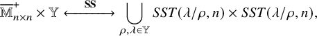
which we denote by
![]() . Moreover, the property
. Moreover, the property
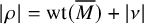 $$ \begin{align} |\rho| = \mathrm{wt}(\overline{M}) + |\nu| \end{align} $$
holds.
4.4 Relations between skew
$\mathbf {RSK}$
and Viennot dynamics

The Viennot dynamics enjoys a very simple relations with the skew $\mathbf {RSK}$
dynamics which we describe in the two propositions below.
$\mathbf {RSK}$
dynamics which we describe in the two propositions below.
Proposition 4.12. Let $\overline {M}^{(t)}, (P_t,Q_t)$
be, respectively, the Viennot and the skew
$\overline {M}^{(t)}, (P_t,Q_t)$
be, respectively, the Viennot and the skew $\mathbf {RSK}$
dynamics with initial data
$\mathbf {RSK}$
dynamics with initial data $\overline {M}^{(1)}=\overline {M}$
and
$\overline {M}^{(1)}=\overline {M}$
and $(P_1,Q_1)=(P,Q)$
. Additionally, assume that
$(P_1,Q_1)=(P,Q)$
. Additionally, assume that $(P,Q) \xrightarrow []{\mathbf {SS} \,} \overline {M}$
. Then
$(P,Q) \xrightarrow []{\mathbf {SS} \,} \overline {M}$
. Then $\overline {M}_{i,j}^{(t)}(k)=m$
if and only if, during the update
$\overline {M}_{i,j}^{(t)}(k)=m$
if and only if, during the update $(P_{-k},Q_{-k}) \to (P_{-k+1},Q_{-k+1})$
, exactly
$(P_{-k},Q_{-k}) \to (P_{-k+1},Q_{-k+1})$
, exactly $m \ i$
-cells of
$m \ i$
-cells of $P_{-k}$
move from row
$P_{-k}$
move from row $t-1$
to row t during the internal insertion of j-cells of
$t-1$
to row t during the internal insertion of j-cells of $Q_{-k}$
.
$Q_{-k}$
.
Proof. This is an immediate consequence of Proposition 3.25.
Proposition 4.13. Let $P,Q\in SST(\lambda /\rho ,n)$
, and define
$P,Q\in SST(\lambda /\rho ,n)$
, and define $(P,Q) \xrightarrow []{\mathbf {SS}\,} \overline {M}$
. Construct tableaux
$(P,Q) \xrightarrow []{\mathbf {SS}\,} \overline {M}$
. Construct tableaux $P',Q'$
shifting up by one unit each cell of
$P',Q'$
shifting up by one unit each cell of $P,Q$
; that is,
$P,Q$
; that is, $P'(c,r)=P(c,r+1)$
and same for
$P'(c,r)=P(c,r+1)$
and same for $Q,Q'$
. Then
$Q,Q'$
. Then $(P',Q')\xrightarrow []{\mathbf {SS}\,} \overline {M}' = \mathbf {V}(\overline {M})$
.
$(P',Q')\xrightarrow []{\mathbf {SS}\,} \overline {M}' = \mathbf {V}(\overline {M})$
.
Proof. Let $(\alpha ,\beta )=\mathrm {rc}(P,Q)$
and
$(\alpha ,\beta )=\mathrm {rc}(P,Q)$
and $(\alpha ',\beta ')=\mathrm {rc}(P',Q')$
. Then, by definition, we have
$(\alpha ',\beta ')=\mathrm {rc}(P',Q')$
. Then, by definition, we have
 $$ \begin{align} \alpha_{i,j}^{\prime} = \alpha_{i,j+1}, \qquad \beta_{i,j}^{\prime} = \beta_{i,j+1}. \end{align} $$
We now construct edge configurations $(\alpha ,\beta ) \mapsto \mathcal {E}$
,
$(\alpha ,\beta ) \mapsto \mathcal {E}$
, $(\alpha ',\beta ') \mapsto \mathcal {E}'$
as in equation (4.6). Thanks to the relation (4.16), it is clear that all edge values of
$(\alpha ',\beta ') \mapsto \mathcal {E}'$
as in equation (4.6). Thanks to the relation (4.16), it is clear that all edge values of $\mathcal {E}'$
will differ by those of
$\mathcal {E}'$
will differ by those of $\mathcal {E}$
by the same shift, or more precisely
$\mathcal {E}$
by the same shift, or more precisely
 $$ \begin{align*}(\mathsf{W}_j^{\prime},\mathsf{S}_j^{\prime},\mathsf{E}_j^{\prime},\mathsf{N}_j^{\prime})(c) = (\mathsf{W}_{j+1},\mathsf{S}_{j+1},\mathsf{E}_{j+1},\mathsf{N}_{j+1})(c), \qquad \text{for all } c \in \mathscr{C}_n, j\in\mathbb{Z}. \end{align*} $$
By equation (4.7) this implies that $\overline {M}' = \mathbf {V}(\overline {M})$
.
$\overline {M}' = \mathbf {V}(\overline {M})$
.
4.5 Asymptotic states of the skew
$\mathbf {RSK}$
dynamics

We describe pairs of tableaux $\mathbf {RSK}^t(P,Q)$
when t becomes large. Contents discussed in this subsection were introduced, along with examples in Section 1.2.
$\mathbf {RSK}^t(P,Q)$
when t becomes large. Contents discussed in this subsection were introduced, along with examples in Section 1.2.
Definition 4.14 (Asymptotic increments).
Let $P,Q\in SST(\lambda /\rho ,n)$
, and consider the skew
$P,Q\in SST(\lambda /\rho ,n)$
, and consider the skew $\mathbf {RSK}$
dynamics
$\mathbf {RSK}$
dynamics $(P_t,Q_t)$
with initial data
$(P_t,Q_t)$
with initial data $(P,Q)$
. We define the asymptotic increment
$(P,Q)$
. We define the asymptotic increment $\mu (P,Q)$
, through its transpose
$\mu (P,Q)$
, through its transpose $\mu '$
as
$\mu '$
as
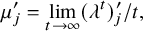 $$ \begin{align} \mu_j^{\prime} = \lim_{t \to \infty} (\lambda^{t})^{\prime}_j/t, \end{align} $$
where $\lambda ^{t}/\rho ^{t}$
is the shape of
$\lambda ^{t}/\rho ^{t}$
is the shape of $P_t,Q_t$
.
$P_t,Q_t$
.
The next proposition justifies the definition of asymptotic increments.
Proposition 4.15. The limits (4.17) exist and numbers $\mu _j^{\prime }$
form a weakly decreasing sequence of integers, defining a partition.
$\mu _j^{\prime }$
form a weakly decreasing sequence of integers, defining a partition.
Proof. Assume that tableaux $P,Q$
are standard, and follow the evolution of the i-cell in
$P,Q$
are standard, and follow the evolution of the i-cell in $P_t$
, for
$P_t$
, for ${t=1,2,\dots }$
, which has coordinate
${t=1,2,\dots }$
, which has coordinate $(c_t,r_t)$
. From the bumping algorithm, it follows that
$(c_t,r_t)$
. From the bumping algorithm, it follows that $r_1<r_2<\cdots $
and also
$r_1<r_2<\cdots $
and also $c_1 \ge c_2 \ge \cdots>0$
. Such weak monotonicity of column coordinates implies that from a certain t onward
$c_1 \ge c_2 \ge \cdots>0$
. Such weak monotonicity of column coordinates implies that from a certain t onward $c_t=c_{t+1}=\cdots $
. Since this holds for any i, it follows that from a certain time
$c_t=c_{t+1}=\cdots $
. Since this holds for any i, it follows that from a certain time $t_*$
onward the content of each column of
$t_*$
onward the content of each column of $P_t$
, for
$P_t$
, for $t>t_*$
, stays constant and
$t>t_*$
, stays constant and $(\lambda ^t)^{\prime }_j = (\lambda ^{t_*})^{\prime }_j + (t-t_*)[(\lambda ^{t_*} )^{\prime }_j - (\rho ^{t_*} )^{\prime }_j ]$
, for all
$(\lambda ^t)^{\prime }_j = (\lambda ^{t_*})^{\prime }_j + (t-t_*)[(\lambda ^{t_*} )^{\prime }_j - (\rho ^{t_*} )^{\prime }_j ]$
, for all $j\ge 1$
. This proves that
$j\ge 1$
. This proves that $\mu _j^{\prime } = (\lambda ^{t_*} )^{\prime }_j - (\rho ^{t_*} )^{\prime }_j$
and they form a sequence of nonnegative integers weakly decreasing in j since
$\mu _j^{\prime } = (\lambda ^{t_*} )^{\prime }_j - (\rho ^{t_*} )^{\prime }_j$
and they form a sequence of nonnegative integers weakly decreasing in j since $(\lambda ^t)^{\prime }_j$
has to remain a weakly decreasing sequence for all t.
$(\lambda ^t)^{\prime }_j$
has to remain a weakly decreasing sequence for all t.
Definition 4.16 (Stable states).
Consider a pair of semistandard tableaux $(P,Q)$
with shape
$(P,Q)$
with shape $\lambda / \rho $
. For
$\lambda / \rho $
. For $t \ge 0$
, let
$t \ge 0$
, let $(P_t,Q_t) = \mathbf {RSK}^t (P,Q)$
and denote their shape by
$(P_t,Q_t) = \mathbf {RSK}^t (P,Q)$
and denote their shape by $\lambda ^{(t)} / \rho ^{(t)} $
and by
$\lambda ^{(t)} / \rho ^{(t)} $
and by $\mu =\mu (P,Q)$
the asymptotic increment. We say that the pair
$\mu =\mu (P,Q)$
the asymptotic increment. We say that the pair $(P,Q)$
is
$(P,Q)$
is $\mathbf {RSK}$
-stable if for all
$\mathbf {RSK}$
-stable if for all $t\ge 0$
we have
$t\ge 0$
we have
 $$ \begin{align} (\lambda^{(t)})'= \lambda ' + t \times \mu' \qquad \text{and} \qquad (\rho^{(t)})' = \rho' + t \times \mu'. \end{align} $$
Reading off columns of pairs of $\mathbf {RSK}$
-stable tableaux, we can associate pairs of vertically strict tableaux.
$\mathbf {RSK}$
-stable tableaux, we can associate pairs of vertically strict tableaux.
Definition 4.17 (Asymptotic vertically strict tableaux).
Let $P,Q \in SST(\lambda /\rho ,n)$
, and consider the skew
$P,Q \in SST(\lambda /\rho ,n)$
, and consider the skew $\mathbf {RSK}$
dynamics
$\mathbf {RSK}$
dynamics $(P_t,Q_t)$
with initial data
$(P_t,Q_t)$
with initial data $(P,Q)$
. Denote by
$(P,Q)$
. Denote by $\mu =\mu (P,Q)$
the asymptotic increment. The asymptotic vertically strict tableaux
$\mu =\mu (P,Q)$
the asymptotic increment. The asymptotic vertically strict tableaux $V,W \in VST(\mu ,n)$
associated to
$V,W \in VST(\mu ,n)$
associated to $(P,Q)$
have j-th column entries given by
$(P,Q)$
have j-th column entries given by
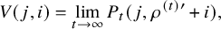 $$ \begin{align} V(j,i) &= \lim_{t\to \infty} P_t( j, \rho^{(t) \prime} +i ),\end{align} $$
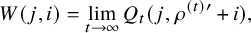 $$ \begin{align} W(j,i) &= \lim_{t\to \infty} Q_t( j, \rho^{(t) \prime} +i ), \end{align} $$
where $\lambda ^{(t)}/\rho ^{(t)}$
denotes the shape of
$\lambda ^{(t)}/\rho ^{(t)}$
denotes the shape of $P_t,Q_t$
.
$P_t,Q_t$
.
Definition 4.18. The projection map
 $$ \begin{align} \Phi : \bigcup_{\rho,\lambda} SST(\lambda/\rho,n) \times SST(\lambda/\rho,n) \to \bigcup_{\mu \in \mathbb{Y}} VST(\mu,n) \times VST(\mu,n) \end{align} $$
assigns to a pair of (generalized) skew tableaux their asymptotic vertically strict tableaux $\Phi :(P,Q) \mapsto (V,W)$
.
$\Phi :(P,Q) \mapsto (V,W)$
.
Remark 4.19. Composing map $\Phi $
with the Sagan–Stanley correspondence would generate a projection
$\Phi $
with the Sagan–Stanley correspondence would generate a projection $\tilde {\Phi }:\overline {\pi } \mapsto (V,W)$
resembling Pak’s asymptotic construction of Shi’s affine Robinson–Schensted’s (RS) correspondence [Reference Shi79]; see [Reference Pak69]. There, pairs of tabloids, along with an array of weights are put in correspondence with periodic permutations, which we can see as weighted permutations
$\tilde {\Phi }:\overline {\pi } \mapsto (V,W)$
resembling Pak’s asymptotic construction of Shi’s affine Robinson–Schensted’s (RS) correspondence [Reference Shi79]; see [Reference Pak69]. There, pairs of tabloids, along with an array of weights are put in correspondence with periodic permutations, which we can see as weighted permutations $\overline {\pi }$
with total weight
$\overline {\pi }$
with total weight $\mathrm {wt}(\overline {\pi })=0$
. In recent works [Reference Chmutov, Frieden, Kim, Lewis and Yudovina19–Reference Chmutov, Pylyavskyy and Yudovina21], authors studied symmetries of the affine RS correspondence which include Knuth relations and crystals. It would be interesting to clarify similarities between projection
$\mathrm {wt}(\overline {\pi })=0$
. In recent works [Reference Chmutov, Frieden, Kim, Lewis and Yudovina19–Reference Chmutov, Pylyavskyy and Yudovina21], authors studied symmetries of the affine RS correspondence which include Knuth relations and crystals. It would be interesting to clarify similarities between projection $\tilde {\Phi }$
, or rather bijection
$\tilde {\Phi }$
, or rather bijection $\tilde {\Upsilon }$
we will introduce in Section 8, and Shi’s affine RS correspondence. We leave this investigation for a future work.
$\tilde {\Upsilon }$
we will introduce in Section 8, and Shi’s affine RS correspondence. We leave this investigation for a future work.
4.6 Asymptotic states of Viennot dynamics
For any fixed weighted biword $\overline {\pi }$
, we aim now to characterize
$\overline {\pi }$
, we aim now to characterize $\mathbf {V}^t(\overline {\pi })$
for large t. To describe the limiting form of such biwords, we need the following definitions.
$\mathbf {V}^t(\overline {\pi })$
for large t. To describe the limiting form of such biwords, we need the following definitions.
Definition 4.20 (Strict down-right loops).
A strict down-right loop $\varsigma $
is a sequence of points
$\varsigma $
is a sequence of points $\varsigma = (\varsigma _j: j = 1,\dots ,J) \subset \mathscr {C}_n$
such that
$\varsigma = (\varsigma _j: j = 1,\dots ,J) \subset \mathscr {C}_n$
such that $\varsigma \subset \xi $
for some down-right loop
$\varsigma \subset \xi $
for some down-right loop $\xi $
and
$\xi $
and
 $$ \begin{align} \varsigma_{k+1} \sim_n \varsigma_k +a_k \mathbf{e}_1 - b_k \mathbf{e}_2, \end{align} $$
for some numbers $a_k,b_k \in \{1,\dots ,n\}$
and
$a_k,b_k \in \{1,\dots ,n\}$
and $k=1,\dots ,J$
. Indices here are taken
$k=1,\dots ,J$
. Indices here are taken $\mod J$
and
$\mod J$
and $\varsigma _{J+1}=\varsigma _1$
. The length of the loop
$\varsigma _{J+1}=\varsigma _1$
. The length of the loop $\varsigma $
is
$\varsigma $
is $\ell (\varsigma )=J$
. Notice that we necessarily have
$\ell (\varsigma )=J$
. Notice that we necessarily have $J\le n$
and that strict down-right loops are ‘localized’ in the sense that
$J\le n$
and that strict down-right loops are ‘localized’ in the sense that $\varsigma $
is always contained in a band
$\varsigma $
is always contained in a band $\{1,\dots ,n\} \times \{ j,\dots ,j+n \} \subset \mathscr {C}_n$
for some
$\{1,\dots ,n\} \times \{ j,\dots ,j+n \} \subset \mathscr {C}_n$
for some $j\in \mathbb {Z}$
.
$j\in \mathbb {Z}$
.
Given a biword $\overline {\pi }$
, written in the usual notation (2.1), we will associate to its columns
$\overline {\pi }$
, written in the usual notation (2.1), we will associate to its columns $\overline {\pi }_i$
points on
$\overline {\pi }_i$
points on $\mathscr {C}_n$
as
$\mathscr {C}_n$
as
 $$ \begin{align} [\overline{\pi}_i] = (q_i, p_i - n w_i) \in \mathscr{C}_n. \end{align} $$
We also denote by $[\overline {\pi }]$
the collections of points
$[\overline {\pi }]$
the collections of points $[\overline {\pi }_i]$
for
$[\overline {\pi }_i]$
for $i=1,\dots , \ell (\overline {\pi })$
. We will confuse at times points
$i=1,\dots , \ell (\overline {\pi })$
. We will confuse at times points $c \in \mathscr {C}_n$
and elements of a weighted biword and write
$c \in \mathscr {C}_n$
and elements of a weighted biword and write $c \in \overline {\pi }$
if
$c \in \overline {\pi }$
if $[\overline {\pi }_i] \sim _n c$
for some i.
$[\overline {\pi }_i] \sim _n c$
for some i.
Definition 4.21 (Localized decreasing sequences).
A weighted biword $\overline {\pi } \in \overline {\mathbb {A}}_{n,n}$
is a localized decreasing sequence, LDS for short, if the set of points
$\overline {\pi } \in \overline {\mathbb {A}}_{n,n}$
is a localized decreasing sequence, LDS for short, if the set of points $([\overline {\pi }_i]:i=1,\dots ,\ell (\overline {\pi }))$
forms a strict down-right loop on
$([\overline {\pi }_i]:i=1,\dots ,\ell (\overline {\pi }))$
forms a strict down-right loop on $\mathscr {C}_n$
.
$\mathscr {C}_n$
.
For the sake of future discussion, we also define increasing sequences on $\mathscr {C}_n$
. They will be used at length in Section 6.
$\mathscr {C}_n$
. They will be used at length in Section 6.
Definition 4.22 (Increasing sequences).
A weighted biword $\overline {\pi } \in \overline {\mathbb {A}}_{n,n}$
is an increasing sequence if the set of points
$\overline {\pi } \in \overline {\mathbb {A}}_{n,n}$
is an increasing sequence if the set of points $([\overline {\pi }_i]:i=1,\dots ,\ell (\overline {\pi }))$
is contained in an up-right path of
$([\overline {\pi }_i]:i=1,\dots ,\ell (\overline {\pi }))$
is contained in an up-right path of $\mathscr {C}_n$
.
$\mathscr {C}_n$
.
If two weighted biwords are such that $\overline {\sigma } \subseteq \overline {\pi }$
we will say that
$\overline {\sigma } \subseteq \overline {\pi }$
we will say that $\overline {\sigma }$
is a subsequence of
$\overline {\sigma }$
is a subsequence of $\overline {\pi }$
. Analogously, we refer to weighted biwords as sequences. An example of a localized decreasing subsequence of a weighted biword is given by
$\overline {\pi }$
. Analogously, we refer to weighted biwords as sequences. An example of a localized decreasing subsequence of a weighted biword is given by
![]() in Figure 12. In the same figure,
in Figure 12. In the same figure,
![]() is an increasing subsequence of
is an increasing subsequence of $\overline {\pi }$
.
$\overline {\pi }$
.
A weighted biword $\overline {\pi }$
viewed as a configuration of points on
$\overline {\pi }$
viewed as a configuration of points on $\mathscr {C}_n$
. Localized decreasing subsequences, as
$\mathscr {C}_n$
. Localized decreasing subsequences, as
![]() form down-right loops around
form down-right loops around $\mathscr {C}_n$
. Increasing subsequences as
$\mathscr {C}_n$
. Increasing subsequences as
![]() form up-right path winding around the cylinder.
form up-right path winding around the cylinder.
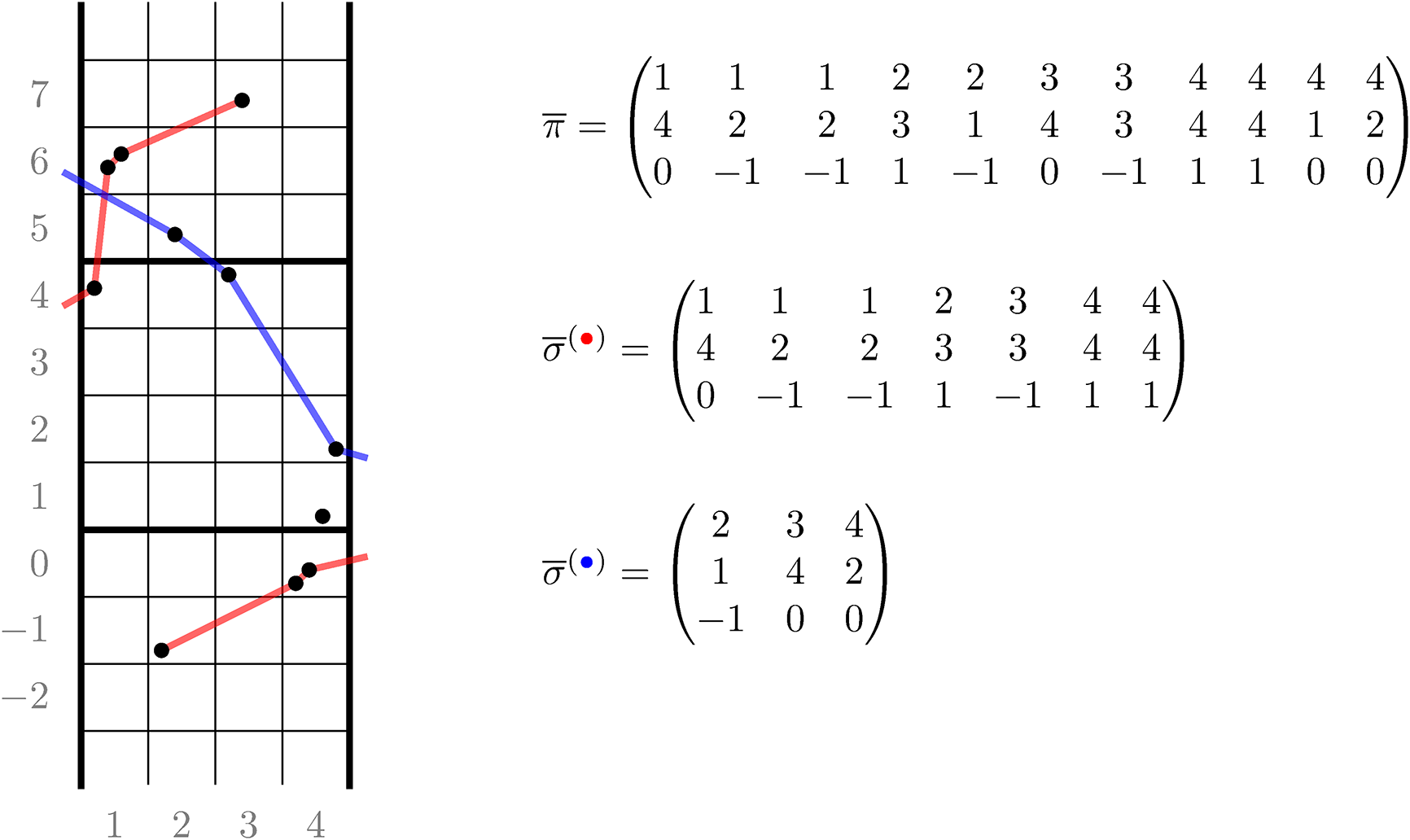
Let us now discuss asymptotic states of the Viennot dynamics. Starting from an initial state $\overline {\pi }$
, it is possible to observe that, after a sufficiently large number of application of the Viennot map, the weighted biword
$\overline {\pi }$
, it is possible to observe that, after a sufficiently large number of application of the Viennot map, the weighted biword $\overline {\pi }^{(t+1)} = \mathbf {V}^t(\overline {\pi })$
separates into subsequences which evolve independently from each other. Drawing the weighted biwords as points on the twisted cylinder, we observe that such subsequences identify clusters of localized decreasing sequences of the same length, as portrayed in Figure 13. This phenomenon is clearly related to the existence of asymptotic states in the skew
$\overline {\pi }^{(t+1)} = \mathbf {V}^t(\overline {\pi })$
separates into subsequences which evolve independently from each other. Drawing the weighted biwords as points on the twisted cylinder, we observe that such subsequences identify clusters of localized decreasing sequences of the same length, as portrayed in Figure 13. This phenomenon is clearly related to the existence of asymptotic states in the skew $\mathbf {RSK}$
dynamics, and we use the interplay between the two dynamics to formalize these observations in the next proposition.
$\mathbf {RSK}$
dynamics, and we use the interplay between the two dynamics to formalize these observations in the next proposition.
Schematic representation of asymptotic state of the Viennot dynamics. For large times t, the point configuration corresponding to $\overline {\pi }^{(t)}$
separates into several clusters of points, each composed of localized decreasing subsequences of the same length. For this reason each cluster evolves with its characteristic speed given by n divided by the length of LDSs in the cluster.
$\overline {\pi }^{(t)}$
separates into several clusters of points, each composed of localized decreasing subsequences of the same length. For this reason each cluster evolves with its characteristic speed given by n divided by the length of LDSs in the cluster.
Proposition 4.23. Let $\overline {\pi } \in \overline {\mathbb {A}}_{n,n}$
. Then there exist
$\overline {\pi } \in \overline {\mathbb {A}}_{n,n}$
. Then there exist $t^* \in \mathbb {N}_0$
and localized decreasing sequences
$t^* \in \mathbb {N}_0$
and localized decreasing sequences $\overline {\xi }^{(1)},\dots ,\overline {\xi }^{(k)}$
such that, for all
$\overline {\xi }^{(1)},\dots ,\overline {\xi }^{(k)}$
such that, for all $t>0$
we have
$t>0$
we have
Moreover, if $\mu =\mu (P,Q)$
is the asymptotic increment of any pair such that
$\mu =\mu (P,Q)$
is the asymptotic increment of any pair such that $(P,Q) \xrightarrow []{\mathbf {SS}\,} \overline {\pi }$
, then, listing the
$(P,Q) \xrightarrow []{\mathbf {SS}\,} \overline {\pi }$
, then, listing the $\overline {\xi }^{(i)}$
’s decreasingly in length, we have
$\overline {\xi }^{(i)}$
’s decreasingly in length, we have $\ell ( \overline {\xi }^{(i)} ) = \mu _i^{\prime }$
for
$\ell ( \overline {\xi }^{(i)} ) = \mu _i^{\prime }$
for $i=1,\dots ,\mu _1$
and in particular
$i=1,\dots ,\mu _1$
and in particular $k=\mu _1$
.
$k=\mu _1$
.
Proof. We are going to use the notion of asymptotic increments for skew tableaux and the relation between skew $\mathbf {RSK}$
dynamics and Viennot dynamics presented in Proposition 4.12. With no loss of generality, we assume that
$\mathbf {RSK}$
dynamics and Viennot dynamics presented in Proposition 4.12. With no loss of generality, we assume that $\overline {\pi }$
is a weighted permutation since such choice simplifies the notation. The general case
$\overline {\pi }$
is a weighted permutation since such choice simplifies the notation. The general case $\overline {\pi } \in \overline {\mathbb {A}}_{n,n}$
is, as usual, recovered by standardization.
$\overline {\pi } \in \overline {\mathbb {A}}_{n,n}$
is, as usual, recovered by standardization.
Let $(P,Q)$
be a pair of standard tableaux such that
$(P,Q)$
be a pair of standard tableaux such that $(P,Q)\xrightarrow []{\mathbf {SS}\,} \overline {\pi }$
, and consider
$(P,Q)\xrightarrow []{\mathbf {SS}\,} \overline {\pi }$
, and consider $(P_t,Q_t)$
the skew
$(P_t,Q_t)$
the skew $\mathbf {RSK}$
dynamics with initial data
$\mathbf {RSK}$
dynamics with initial data $(P,Q)$
. Let
$(P,Q)$
. Let $T\in \mathbb {N}$
be large enough so that the pair
$T\in \mathbb {N}$
be large enough so that the pair $(P_T,Q_T)$
is
$(P_T,Q_T)$
is $\mathbf {RSK}$
-stable, and call
$\mathbf {RSK}$
-stable, and call $\mu =\mu (P,Q)$
its asymptotic increment. Let
$\mu =\mu (P,Q)$
its asymptotic increment. Let $0=R_0, R_1,R_2,\dots $
define a rectangular decomposition of
$0=R_0, R_1,R_2,\dots $
define a rectangular decomposition of $\mu $
as in equation (2.9), and set
$\mu $
as in equation (2.9), and set $r_i=R_i - R_{i-1}$
. Then, when
$r_i=R_i - R_{i-1}$
. Then, when $t \ge T$
, during the update
$t \ge T$
, during the update $(P_t,Q_t) \to (P_{t+1},Q_{t+1})$
columns
$(P_t,Q_t) \to (P_{t+1},Q_{t+1})$
columns $R_{i-1}+1,\dots ,R_{i}$
are shifted down by
$R_{i-1}+1,\dots ,R_{i}$
are shifted down by $\mu _{R_i}^{\prime }$
cells. If
$\mu _{R_i}^{\prime }$
cells. If $\lambda / \rho $
is the skew shape of
$\lambda / \rho $
is the skew shape of $(P_T,Q_T)$
, the vertical displacement between labeled boxes at columns
$(P_T,Q_T)$
, the vertical displacement between labeled boxes at columns $R_i$
and
$R_i$
and $R_i+1$
can be assumed to be arbitrarily large, or in other words
$R_i+1$
can be assumed to be arbitrarily large, or in other words $\rho _{R_i}^{\prime } \gg \lambda _{R_i+1}^{\prime }$
, choosing T sufficiently large.
$\rho _{R_i}^{\prime } \gg \lambda _{R_i+1}^{\prime }$
, choosing T sufficiently large.
Consider an integer $K> \lambda _1^{\prime }$
. Then by choosing K large enough there exist times
$K> \lambda _1^{\prime }$
. Then by choosing K large enough there exist times $T_1 < T_2 <\cdots $
, with
$T_1 < T_2 <\cdots $
, with $T<T_1$
, such that in the skew shape of
$T<T_1$
, such that in the skew shape of $(P_{T_i},Q_{T_i})$
columns
$(P_{T_i},Q_{T_i})$
columns $1, \dots , R_i$
have only cells with a row coordinate larger than K, while cells at columns
$1, \dots , R_i$
have only cells with a row coordinate larger than K, while cells at columns $R_i+1,R_i+2,\dots $
have a row coordinate smaller than K. By choosing K large enough, we can assume that the differences
$R_i+1,R_i+2,\dots $
have a row coordinate smaller than K. By choosing K large enough, we can assume that the differences $T_{i+1}-T_{i}$
are arbitrarily large.
$T_{i+1}-T_{i}$
are arbitrarily large.
Consider now the Viennot dynamics $\overline {\pi }^{(t)}$
with initial data
$\overline {\pi }^{(t)}$
with initial data $\overline {\pi }$
. Recall that, by Proposition 4.12, the weighted permutation
$\overline {\pi }$
. Recall that, by Proposition 4.12, the weighted permutation $\overline {\pi }^{(K)}$
encodes the times at which specific entries of
$\overline {\pi }^{(K)}$
encodes the times at which specific entries of $(P,Q)$
reach the K-th row during the skew
$(P,Q)$
reach the K-th row during the skew $\mathbf {RSK}$
dynamics. By the discussion above, taking
$\mathbf {RSK}$
dynamics. By the discussion above, taking $T_1,T_2,\dots $
sufficiently large and spread apart we find that
$T_1,T_2,\dots $
sufficiently large and spread apart we find that $\overline {\pi }^{(K)}$
can be written as
$\overline {\pi }^{(K)}$
can be written as
![]() , where
, where $\overline {\sigma }^{(j)}$
’s are weighted biwords encoding information about columns of length
$\overline {\sigma }^{(j)}$
’s are weighted biwords encoding information about columns of length $\mu _{R_j}^{\prime }$
of
$\mu _{R_j}^{\prime }$
of $(P_T,Q_T)$
. More in detail, denoting
$(P_T,Q_T)$
. More in detail, denoting
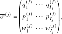
we have $I_j = \mu _{R_j}^{\prime } r_j$
and
$I_j = \mu _{R_j}^{\prime } r_j$
and $\max _{1\le i \le I_j} w_i^{(j)} \ll \min _{1\le i \le I_{j-1}} w_i^{(j-1)}$
. By stability of
$\max _{1\le i \le I_j} w_i^{(j)} \ll \min _{1\le i \le I_{j-1}} w_i^{(j-1)}$
. By stability of $(P_T,Q_T)$
, we can also conclude that under the action of Viennot map,
$(P_T,Q_T)$
, we can also conclude that under the action of Viennot map, $\overline {\sigma }^{(1)}, \overline {\sigma }^{(2)}, \dots $
evolve independently from each other, or in other words
$\overline {\sigma }^{(1)}, \overline {\sigma }^{(2)}, \dots $
evolve independently from each other, or in other words
for all $s \ge 0$
. To prove our proposition, we need to show that there exist LDSs
$s \ge 0$
. To prove our proposition, we need to show that there exist LDSs $\overline {\xi }^{(j,1)} ,\dots , \overline {\xi }^{(j,r_j)}$
such that
$\overline {\xi }^{(j,1)} ,\dots , \overline {\xi }^{(j,r_j)}$
such that
![]() , having length
, having length $\ell ( \overline {\xi }^{(j,r)} ) = \mu _{R_j}^{\prime }$
for
$\ell ( \overline {\xi }^{(j,r)} ) = \mu _{R_j}^{\prime }$
for $1\leq r \leq r_j$
and that evolve autonomously under Viennot dynamics
$1\leq r \leq r_j$
and that evolve autonomously under Viennot dynamics
Figure 13 helps us visualize the quantities defined above. Namely, the $\overline {\sigma }^{(j)}$
’s correspond to different clusters of the point configuration, whereas the
$\overline {\sigma }^{(j)}$
’s correspond to different clusters of the point configuration, whereas the $\overline {\xi }^{(j,r)}$
’s will be the localized decreasing subsequences of length
$\overline {\xi }^{(j,r)}$
’s will be the localized decreasing subsequences of length $\mu _{R_j}^{\prime }$
forming each cluster.
$\mu _{R_j}^{\prime }$
forming each cluster.
We now use Proposition 4.12. For any j such that $r_j>0$
let
$r_j>0$
let $c\in \{R_{j-1}+1 ,\dots , R_j \}$
and denote
$c\in \{R_{j-1}+1 ,\dots , R_j \}$
and denote $\mu _{R_j}^{\prime }=m$
. Let
$\mu _{R_j}^{\prime }=m$
. Let $p_1<\cdots <p_m$
and
$p_1<\cdots <p_m$
and $q_1 <\dots < q_m$
be entries of c-th columns of
$q_1 <\dots < q_m$
be entries of c-th columns of $P_t,Q_t$
for t large enough. Let
$P_t,Q_t$
for t large enough. Let $\widetilde {t}\in \{ T_{j-1}+1,\dots ,T_j \}$
be the first time
$\widetilde {t}\in \{ T_{j-1}+1,\dots ,T_j \}$
be the first time $p_m$
reaches a row greater than K. Since columns evolve autonomously in stable states, the only possibility is that
$p_m$
reaches a row greater than K. Since columns evolve autonomously in stable states, the only possibility is that $p_m$
reached row K as a result of the internal insertion at cell corresponding to the
$p_m$
reached row K as a result of the internal insertion at cell corresponding to the $q_s$
-cell in
$q_s$
-cell in $Q_{\widetilde {t}-1}$
for some
$Q_{\widetilde {t}-1}$
for some $s\in \{1,\dots ,m\}$
. Moreover, internal insertion corresponding to
$s\in \{1,\dots ,m\}$
. Moreover, internal insertion corresponding to $q_{s+1},\dots , q_m$
during the update will result in
$q_{s+1},\dots , q_m$
during the update will result in $p_{m-1},\dots ,p_{s}$
reaching row K. This implies that
$p_{m-1},\dots ,p_{s}$
reaching row K. This implies that $(q_S,p_{m+s-S} + n \widetilde {t} \,) \in [\overline {\sigma }^{(j)}]$
for all
$(q_S,p_{m+s-S} + n \widetilde {t} \,) \in [\overline {\sigma }^{(j)}]$
for all $S=s,\dots , m$
. During the update
$S=s,\dots , m$
. During the update $(P_{\, \widetilde {t}},Q_{ \, \widetilde {t}}) \to (P_{\, \widetilde {t}+1},Q_{\, \widetilde {t}+1})$
the remaining cells
$(P_{\, \widetilde {t}},Q_{ \, \widetilde {t}}) \to (P_{\, \widetilde {t}+1},Q_{\, \widetilde {t}+1})$
the remaining cells $p_1,\dots ,p_{s-1}$
will reach row K and they will do so in correspondence of internal insertion of
$p_1,\dots ,p_{s-1}$
will reach row K and they will do so in correspondence of internal insertion of $q_1,\dots , q_{s-1}$
-cells in
$q_1,\dots , q_{s-1}$
-cells in $Q_{\widetilde {t}}$
. Therefore, also
$Q_{\widetilde {t}}$
. Therefore, also $(q_S,p_S + n (\widetilde {t}+1) \,) \in [\overline {\sigma }^{(j)}]$
for all
$(q_S,p_S + n (\widetilde {t}+1) \,) \in [\overline {\sigma }^{(j)}]$
for all $S=1,\dots , s-1$
and this implies that
$S=1,\dots , s-1$
and this implies that
 $$ \begin{align*} [\overline{\xi}^{(j,1)}] = (q_1,p_1 + n (\widetilde{t}+1)) \to \cdots &\to (q_{s-1},p_{s-1} + n (\widetilde{t}+1)) \\ &\qquad\qquad\qquad\qquad\to (q_s,p_1 + n \widetilde{t}) \to \cdots \to (q_m , p_{s} + n \widetilde{t}) \end{align*} $$
is a strict down-right loop identifying a subsequence of $\overline {\sigma }^{(j)}$
. Repeating the argument for all columns
$\overline {\sigma }^{(j)}$
. Repeating the argument for all columns $c=R_{j-1}+1,\dots , R_j$
, we find disjoint localized decreasing subsequences of
$c=R_{j-1}+1,\dots , R_j$
, we find disjoint localized decreasing subsequences of $\overline {\sigma }^{(j)}$
, which we might denote by
$\overline {\sigma }^{(j)}$
, which we might denote by $\overline {\xi }^{(j,1)},\dots , \overline {\xi }^{(j,r_j)}$
, all having length equal to
$\overline {\xi }^{(j,1)},\dots , \overline {\xi }^{(j,r_j)}$
, all having length equal to $\mu _{R_j}^{\prime }$
. One also easily sees that since columns of tableaux
$\mu _{R_j}^{\prime }$
. One also easily sees that since columns of tableaux $(P_t,Q_t)$
evolve autonomously, then also the corresponding LDSs
$(P_t,Q_t)$
evolve autonomously, then also the corresponding LDSs $\xi ^{(j,r)}$
evolve independently under Viennot map and this completes the proof.
$\xi ^{(j,r)}$
evolve independently under Viennot map and this completes the proof.
5 Affine crystal structures
In this section, we first review basic notions in the theory of Kashiwara crystals, focusing only on the type $A^{(1)}_{n-1}$
case. Many of the objects encountered in the previous sections possess affine bicrystal graph structures, such as the set of pairs
$A^{(1)}_{n-1}$
case. Many of the objects encountered in the previous sections possess affine bicrystal graph structures, such as the set of pairs $(V,W)$
of vertically strict tableaux, the set of pairs
$(V,W)$
of vertically strict tableaux, the set of pairs $(P,Q)$
of semistandard tableaux or the set of matrices
$(P,Q)$
of semistandard tableaux or the set of matrices $\overline {\mathbb {M}}_{n\times n}$
. Vertically strict tableaux are a standard combinatorial model of an affine (bi)crystal, whereas the affine bicrystal structure on pairs
$\overline {\mathbb {M}}_{n\times n}$
. Vertically strict tableaux are a standard combinatorial model of an affine (bi)crystal, whereas the affine bicrystal structure on pairs $(P,Q)$
or on matrices
$(P,Q)$
or on matrices $\overline {M}$
described in Sections 5.4 and 5.5 is new. The main result of this section is given by Proposition 5.7, which asserts the
$\overline {M}$
described in Sections 5.4 and 5.5 is new. The main result of this section is given by Proposition 5.7, which asserts the $\widehat {\mathfrak {sl}}_n$
bicrystal symmetry of the skew
$\widehat {\mathfrak {sl}}_n$
bicrystal symmetry of the skew $\mathbf {RSK}$
map. This symmetry will allow to characterize the skew
$\mathbf {RSK}$
map. This symmetry will allow to characterize the skew $\mathbf {RSK}$
dynamics completely in later sections; see Proposition 5.8.
$\mathbf {RSK}$
dynamics completely in later sections; see Proposition 5.8.
5.1 Crystals and bicrystals
Most of the material in this subsection is contained in [Reference Bump and Schilling16, Reference Hong and Kang42]. For a short introductory account on the subject, the reader may consult [Reference Shimozono81].
An $\widehat {\mathfrak {sl}}_n$
crystal graph
Footnote
5
, or equivalently for us an affine crystal graph, is a set of vertices B, equipped with a function
$\widehat {\mathfrak {sl}}_n$
crystal graph
Footnote
5
, or equivalently for us an affine crystal graph, is a set of vertices B, equipped with a function $\gamma : B \to \mathbb {N}_0^n$
(commonly referred to as weight, but here called content), and colored directed edges
$\gamma : B \to \mathbb {N}_0^n$
(commonly referred to as weight, but here called content), and colored directed edges $b \xrightarrow []{i} b'$
, with colors i ranging in
$b \xrightarrow []{i} b'$
, with colors i ranging in $\{ 0,\dots ,n-1 \}$
satisfying the following two properties.
$\{ 0,\dots ,n-1 \}$
satisfying the following two properties.
-
1. There are no multiple edges. In case
$b \xrightarrow []{i} b'$
, we write where
$$ \begin{align*} b' = \widetilde{f}_{i}(b), \qquad \text{or} \qquad b=\widetilde{e}_{i}(b'), \end{align*} $$
$\widetilde {f}_{i},\widetilde {e}_{i}$
are, respectively, the i-th lowering and raising Kashiwara operators. When
$\widetilde {f}_{i}$
is not defined for an element b we will write
$\widetilde {f}_{i}(b)=\varnothing $
and similarly for
$\widetilde {e}_{i}$
. Kashiwara operators define numbers
$\varphi _i,\varepsilon _i : B \to \mathbb {N}_0$
as
$$ \begin{gather*} \varphi_i(b) = \max\{m : \widetilde{f}_{i}^m(b) \neq \varnothing \}, \\ \varepsilon_i(b) = \max\{m : \widetilde{e}_{i}^{\,m}(b) \neq \varnothing \}. \end{gather*} $$
-
2. Let
$h_0=\mathbf {e}_n - \mathbf {e}_{1}$
and
$h_i = \mathbf {e}_i - \mathbf {e}_{i+1}$
,
$i=1,\dots ,n-1$
. Then, for all
$b\in B$
we have and, whenever
$$ \begin{align*} \langle h_i , \gamma(b) \rangle = \varphi_i(b) - \varepsilon_i (b) \end{align*} $$
$\widetilde {f}_{i}(b)\neq \varnothing $
, we have Here,
$$ \begin{align*} \gamma (\widetilde{f}_{i}(b)) = \gamma(b) - h_i. \end{align*} $$
$\mathbf {e}_i$
and
$\langle \cdot , \cdot \rangle $
are, respectively, the standard basis and the standard scalar product of
$\mathbb {C}^n$
.


The set B in this case is called crystal, but unless necessary we will not distinguish between the notion of crystal and its graph. An example of an affine crystal graph is reported in Figure 18 below. We also define $\mathfrak {sl}_n$
crystals graphs, which we refer to as classical crystals graphs, removing from the description above all statements concerning
$\mathfrak {sl}_n$
crystals graphs, which we refer to as classical crystals graphs, removing from the description above all statements concerning $0$
-edges. For instance, in Figure 18 the classical crystal graph is given erasing red and blue edges.
$0$
-edges. For instance, in Figure 18 the classical crystal graph is given erasing red and blue edges.
Lowering and raising operators $\widetilde {f}_{i},\widetilde {e}_{i}$
are partial mutual inverses; that is, if
$\widetilde {f}_{i},\widetilde {e}_{i}$
are partial mutual inverses; that is, if $\widetilde {e}_{i}(b) \neq \varnothing $
, then
$\widetilde {e}_{i}(b) \neq \varnothing $
, then $\widetilde {f}_{i}\circ \widetilde {e}_{i}(b)=b$
and same for the opposite case. For this reason, in case h is an operator written as
$\widetilde {f}_{i}\circ \widetilde {e}_{i}(b)=b$
and same for the opposite case. For this reason, in case h is an operator written as
 $$ \begin{align*} h=(\widetilde{e}_{i_1})^{N_1} \circ (\widetilde{f}_{i_2})^{N_2} \circ \cdots \circ (\widetilde{e}_{i_{k-1}})^{N_{k-1}} \circ (\widetilde{f}_{i_k})^{N_k}, \end{align*} $$
then we will denote by $h^{-1}$
the operator
$h^{-1}$
the operator
 $$ \begin{align*} h^{-1} = (\widetilde{e}_{i_k})^{N_k} \circ (\widetilde{f}_{i_{k-1}})^{N_{k-1}} \circ \cdots \circ (\widetilde{e}_{i_2})^{N_2} \circ (\widetilde{f}_{i_1})^{N_1}. \end{align*} $$
Clearly, if $h(b)\neq \varnothing $
, then
$h(b)\neq \varnothing $
, then $h^{-1}\circ h(b) =b$
.
$h^{-1}\circ h(b) =b$
.
An $\widehat {\mathfrak {sl}}_n$
bicrystal graph is a set of vertices B possessing two commuting
$\widehat {\mathfrak {sl}}_n$
bicrystal graph is a set of vertices B possessing two commuting $\widehat {\mathfrak {sl}}_n$
crystal graph structures, that is, two commuting families of Kashiwara operators. We will denote the two sets of Kashiwara operators for bicrystals with the notation
$\widehat {\mathfrak {sl}}_n$
crystal graph structures, that is, two commuting families of Kashiwara operators. We will denote the two sets of Kashiwara operators for bicrystals with the notation $\widetilde {E}^{(1)}_i, \widetilde {F}^{(1)}_i$
and
$\widetilde {E}^{(1)}_i, \widetilde {F}^{(1)}_i$
and $\widetilde {E}^{(2)}_i, \widetilde {F}^{(2)}_i$
,
$\widetilde {E}^{(2)}_i, \widetilde {F}^{(2)}_i$
, $i=0,\dots ,n-1$
. For instance, if B is an
$i=0,\dots ,n-1$
. For instance, if B is an $\widehat {\mathfrak {sl}}_n$
crystal, then the Cartesian product
$\widehat {\mathfrak {sl}}_n$
crystal, then the Cartesian product $B \times B$
is an
$B \times B$
is an $\widehat {\mathfrak {sl}}_n$
bicrystal setting
$\widehat {\mathfrak {sl}}_n$
bicrystal setting
 $$ \begin{align} \widetilde{E}^{(1)}_i = \widetilde{e}_{i} \times \mathbf{1}, \qquad \widetilde{E}^{(2)}_i = \mathbf{1} \times \widetilde{e}_{i}, \qquad \widetilde{F}^{(1)}_i = \widetilde{f}_{i} \times \mathbf{1}, \qquad \widetilde{F}^{(2)}_i = \mathbf{1} \times \widetilde{f}_{i}, \end{align} $$
and letting content function $\gamma $
act independently on single components. We will introduce below a more elaborate example of bicrystal. Also, in the case of bicrystals we will adopt the same convention as above for inverse operators. If h is a combinations of Kashiwara operators
$\gamma $
act independently on single components. We will introduce below a more elaborate example of bicrystal. Also, in the case of bicrystals we will adopt the same convention as above for inverse operators. If h is a combinations of Kashiwara operators $\widetilde {E}^{(\epsilon )}_i, \widetilde {F}^{(\epsilon )}_i$
, then
$\widetilde {E}^{(\epsilon )}_i, \widetilde {F}^{(\epsilon )}_i$
, then $h^{-1}$
will be the operator obtained reading the expansion of h backward and substituting each
$h^{-1}$
will be the operator obtained reading the expansion of h backward and substituting each $\widetilde {E}^{(\epsilon )}_i$
with
$\widetilde {E}^{(\epsilon )}_i$
with $\widetilde {F}^{(\epsilon )}_i$
and vice versa.
$\widetilde {F}^{(\epsilon )}_i$
and vice versa.
Definition 5.1. Let $\mathfrak {g}$
be either
$\mathfrak {g}$
be either $\mathfrak {sl}_n$
or
$\mathfrak {sl}_n$
or $\widehat {\mathfrak {sl}}_n$
and
$\widehat {\mathfrak {sl}}_n$
and $B,B'$
be
$B,B'$
be $\mathfrak {g}$
crystals. A map
$\mathfrak {g}$
crystals. A map $\phi : B \to B'$
is a morphism of crystals if
$\phi : B \to B'$
is a morphism of crystals if
 $$ \begin{align} \phi \circ \widetilde{e}_{i} = \widetilde{e}_{i} \circ \phi, \qquad \phi \circ \widetilde{f}_{i} = \widetilde{f}_{i} \circ \phi \qquad \text{for all }i=0,\dots,n-1 \end{align} $$
and $\gamma (\phi (b)) = \gamma (b)$
for all
$\gamma (\phi (b)) = \gamma (b)$
for all $b\in B$
. An isomorphism of crystals is a bijective morphism of crystals whose inverse is also a morphism of crystals. We use the convention that
$b\in B$
. An isomorphism of crystals is a bijective morphism of crystals whose inverse is also a morphism of crystals. We use the convention that $\phi (\varnothing )=\varnothing $
.
$\phi (\varnothing )=\varnothing $
.
Analogously, we define a morphism of affine bicrystals $B,B'$
as a map
$B,B'$
as a map $\phi :B\to B'$
that is a morphism of crystal for both crystal graphs structures. If
$\phi :B\to B'$
that is a morphism of crystal for both crystal graphs structures. If $\phi $
is invertible and its inverse is a morphism of bicrystals, then
$\phi $
is invertible and its inverse is a morphism of bicrystals, then $\phi $
is an isomorphism of bicrystals.
$\phi $
is an isomorphism of bicrystals.
5.2 Classical Kashiwara operators
On the set of words $\mathcal {A}_n^*$
, we can define the action of Kashiwara operators
$\mathcal {A}_n^*$
, we can define the action of Kashiwara operators $\widetilde {e}_{i}, \widetilde {f}_{i}$
for
$\widetilde {e}_{i}, \widetilde {f}_{i}$
for $i=1,\dots , n-1$
. The raising operator
$i=1,\dots , n-1$
. The raising operator $\widetilde {e}_{i}$
acts replacing an entry
$\widetilde {e}_{i}$
acts replacing an entry $i+1$
with i following the so-called signature rule. It goes as follows:
$i+1$
with i following the so-called signature rule. It goes as follows:
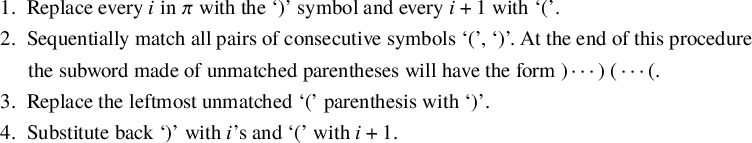 $$ \begin{align} \begin{aligned}&1.\ \text{ Replace every } i \text{ in } \pi \text{ with the `)' symbol and every } i+1 \text{ with `('}.\\&2.\ \text{ Sequentially match all pairs of consecutive symbols `(', `)'. At the end of this procedure}\\&\quad\kern1pt\ \text{the subword made of unmatched parentheses will have the form )} \cdots \text{) (} \cdots \text{(}.\\&3.\ \text{ Replace the leftmost unmatched `(' parenthesis with `)'}.\\&4.\ \text{ Substitute back `)' with } i\text{'s and `(' with } i+1. \end{aligned} \end{align} $$
Sometimes, this operation is impossible (e.g., when $\pi \in \mathcal {A}_n^*$
has no
$\pi \in \mathcal {A}_n^*$
has no $(i+1)$
’s) and in that case we impose
$(i+1)$
’s) and in that case we impose $\widetilde {e}_{i}(\pi ) = \varnothing $
.
$\widetilde {e}_{i}(\pi ) = \varnothing $
.
The lowering operator $\widetilde {f}_{i}$
is defined analogously to
$\widetilde {f}_{i}$
is defined analogously to $\widetilde {e}_{i}$
with the difference that the third step of equation (5.3) becomes
$\widetilde {e}_{i}$
with the difference that the third step of equation (5.3) becomes
 $$ \begin{align} (3')\ \text{Replace the rightmost unmatched `)' parenthesis with `('}. \end{align} $$
As before, when the procedure is impossible we set $\widetilde {f}_{i}(\pi )=\varnothing $
. It is easy to see that
$\widetilde {f}_{i}(\pi )=\varnothing $
. It is easy to see that $\widetilde {e}_{i}$
and
$\widetilde {e}_{i}$
and $\widetilde {f}_{i}$
are mutual inverses, when both their operations are defined. We illustrate the action of Kashiwara operators with an example. Here,
$\widetilde {f}_{i}$
are mutual inverses, when both their operations are defined. We illustrate the action of Kashiwara operators with an example. Here, $i=2$
:
$i=2$
:
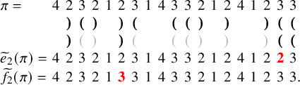
In the third line, matched parentheses were drawn in light gray, while in the last two lines we highlighted in red the letters of $\pi $
that were changed by
$\pi $
that were changed by $\widetilde {e}_{2}$
and
$\widetilde {e}_{2}$
and $\widetilde {f}_{2}$
.
$\widetilde {f}_{2}$
.
The action of Kashiwara operators endows the set $\mathcal {A}_n^*$
with an
$\mathcal {A}_n^*$
with an $\mathfrak {sl}_n$
crystal graph structure, the content
$\mathfrak {sl}_n$
crystal graph structure, the content $\gamma $
being defined as in Section 2.1. For any word
$\gamma $
being defined as in Section 2.1. For any word $\pi $
,
$\pi $
, $\varphi _i(\pi )$
counts the number of unmatched
$\varphi _i(\pi )$
counts the number of unmatched $\text {`)'}$
parentheses we find while computing the action of i-th Kashiwara operators on
$\text {`)'}$
parentheses we find while computing the action of i-th Kashiwara operators on $\pi $
and
$\pi $
and $\varepsilon _i(\pi )$
is the number of unmatched
$\varepsilon _i(\pi )$
is the number of unmatched $\text {`('}$
parentheses. For instance in equation (5.5),
$\text {`('}$
parentheses. For instance in equation (5.5), $\varphi _2(\pi ) = \varepsilon _2(\pi ) =2$
.
$\varphi _2(\pi ) = \varepsilon _2(\pi ) =2$
.
The action of Kashiwara operators extends to the set of semistandard tableaux. If $P\in SST(\lambda / \mu , n)$
, denoting
$P\in SST(\lambda / \mu , n)$
, denoting $\pi _P^{\mathrm {col}}$
its column reading word, we define
$\pi _P^{\mathrm {col}}$
its column reading word, we define $\widetilde {e}_{i}(P)$
as the tableaux with shape
$\widetilde {e}_{i}(P)$
as the tableaux with shape $\lambda /\mu $
and column reading word
$\lambda /\mu $
and column reading word $\widetilde {e}_{i}(\pi _P^{\mathrm {col}})$
. The action of
$\widetilde {e}_{i}(\pi _P^{\mathrm {col}})$
. The action of $\widetilde {f}_{i}$
is defined equivalently. For example, we have
$\widetilde {f}_{i}$
is defined equivalently. For example, we have
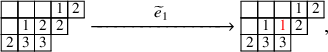
where we highlighted in red the cell that changed its label.
The study of $\mathfrak {sl}_n$
crystal structure of the set of semistandard tableaux has a long history rooted in the seminal paper [Reference Robinson72]. In fact, as recalled in [Reference Shimozono81], the first instance of the RSK correspondence, was realized by Robinson imposing that map
$\mathfrak {sl}_n$
crystal structure of the set of semistandard tableaux has a long history rooted in the seminal paper [Reference Robinson72]. In fact, as recalled in [Reference Shimozono81], the first instance of the RSK correspondence, was realized by Robinson imposing that map $\pi \mapsto P$
would commute with the action of
$\pi \mapsto P$
would commute with the action of $\widetilde {e}_{i},\widetilde {f}_{i}$
. In general, Kashiwara operators are coplactic transformations, which means that they commute with jeu de taquin moves; see Appendix A.1. This known result is stated in the following proposition. In order to make the text self-contained all ingredients necessary to its proof, along with a short review of theory of Knuth relations, are reported in Appendix A.
$\widetilde {e}_{i},\widetilde {f}_{i}$
. In general, Kashiwara operators are coplactic transformations, which means that they commute with jeu de taquin moves; see Appendix A.1. This known result is stated in the following proposition. In order to make the text self-contained all ingredients necessary to its proof, along with a short review of theory of Knuth relations, are reported in Appendix A.
Proposition 5.2. Let h be an operator in the set $\{\widetilde {e}_{1}, \widetilde {f}_{1}, \dots ,\widetilde {e}_{n-1}, \widetilde {f}_{n-1}\}$
and let P be a semistandard tableau. Then for any transformation J that performs a sequence of jeu de taquin slides we have
$\{\widetilde {e}_{1}, \widetilde {f}_{1}, \dots ,\widetilde {e}_{n-1}, \widetilde {f}_{n-1}\}$
and let P be a semistandard tableau. Then for any transformation J that performs a sequence of jeu de taquin slides we have $h(J(P)) = J(h(P))$
.
$h(J(P)) = J(h(P))$
.
Proof. Combining Proposition A.7 and Proposition A.9 (1) we find that $h(J(P)) \stackrel {*}{\simeq } J(h(P))$
. On the other hand, thanks to Proposition A.2 and Proposition A.9 (2) we have
$h(J(P)) \stackrel {*}{\simeq } J(h(P))$
. On the other hand, thanks to Proposition A.2 and Proposition A.9 (2) we have $h(J(P)) \simeq J(h(P))$
. Therefore,
$h(J(P)) \simeq J(h(P))$
. Therefore, $h(J(P)) = J(h(P))$
by Proposition A.8.
$h(J(P)) = J(h(P))$
by Proposition A.8.
We will utilize result of Proposition 5.2 in a slightly weaker form reported next. Recall that $\mathcal {R}_{[r]}$
denotes the internal insertion.
$\mathcal {R}_{[r]}$
denotes the internal insertion.
Corollary 5.3. Let h be an operator in the set $\{\widetilde {e}_{1}, \widetilde {f}_{1}, \dots ,\widetilde {e}_{n-1}, \widetilde {f}_{n-1}\}$
, and let P be a semistandard tableau. Then for all
$\{\widetilde {e}_{1}, \widetilde {f}_{1}, \dots ,\widetilde {e}_{n-1}, \widetilde {f}_{n-1}\}$
, and let P be a semistandard tableau. Then for all $r\in \mathbb {Z}$
we have
$r\in \mathbb {Z}$
we have $h \circ \mathcal {R}_{[r]}(P) = \mathcal {R}_{[r]} \circ h (P)$
.
$h \circ \mathcal {R}_{[r]}(P) = \mathcal {R}_{[r]} \circ h (P)$
.


5.3 Vertically strict tableaux as affine crystals
Denote by $B^{r,1}$
the set of semistandard Young tableaux of single column shape
$B^{r,1}$
the set of semistandard Young tableaux of single column shape $1^r$
and entries from
$1^r$
and entries from $\mathcal {A}_n$
. Following [Reference Shimozono80], on
$\mathcal {A}_n$
. Following [Reference Shimozono80], on $B^{r,1}$
we define the
$B^{r,1}$
we define the $0$
-th Kashiwara operators
$0$
-th Kashiwara operators $\widetilde {e}_{0}, \widetilde {f}_{0}$
as
$\widetilde {e}_{0}, \widetilde {f}_{0}$
as
 $$ \begin{align} \widetilde{e}_{0} = \mathrm{pr}^{-1} \circ \widetilde{e}_{1} \circ \mathrm{pr} \qquad \text{and} \qquad \widetilde{f}_{0} = \mathrm{pr}^{-1} \circ \widetilde{f}_{1} \circ \mathrm{pr}, \end{align} $$
where $\mathrm {pr}$
is the promotion operator. For any
$\mathrm {pr}$
is the promotion operator. For any $b \in B^{r,1}$
, its promotion
$b \in B^{r,1}$
, its promotion $b'=\mathrm {pr}(b) \in B^{r,1}$
is the only tableau with content
$b'=\mathrm {pr}(b) \in B^{r,1}$
is the only tableau with content $\gamma _i(b') = \gamma _{i-1}(b)$
, where indices i are taken
$\gamma _i(b') = \gamma _{i-1}(b)$
, where indices i are taken $\mod n$
. In words,
$\mod n$
. In words, $\widetilde {e}_{0}(b)$
is obtained replacing the 1-cell of b with an n-cell and reordering the result. For example, if
$\widetilde {e}_{0}(b)$
is obtained replacing the 1-cell of b with an n-cell and reordering the result. For example, if $n=6$
, we have
$n=6$
, we have
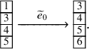
Such operation is impossible if b has an n-cell or if it does not have a $1$
-cell, in which cases we set
$1$
-cell, in which cases we set $\widetilde {e}_{0}(b)=\varnothing $
. An analogous description may be given for
$\widetilde {e}_{0}(b)=\varnothing $
. An analogous description may be given for $\widetilde {f}_{0}$
. By convention, we define
$\widetilde {f}_{0}$
. By convention, we define $B^{0,1} = \{ \mathbf {0} \}$
and we assume
$B^{0,1} = \{ \mathbf {0} \}$
and we assume $\widetilde {e}_{i},\widetilde {f}_{i}:\mathbf {0}\to \varnothing $
, for all
$\widetilde {e}_{i},\widetilde {f}_{i}:\mathbf {0}\to \varnothing $
, for all $i=0,\dots ,n-1$
and
$i=0,\dots ,n-1$
and $\mathrm {pr}(\mathbf {0}) = \mathbf {0}$
. Naturally, the column word of
$\mathrm {pr}(\mathbf {0}) = \mathbf {0}$
. Naturally, the column word of $\mathbf {0}$
is the empty word.
$\mathbf {0}$
is the empty word.
For any composition $\varkappa =(\varkappa _1, \dots , \varkappa _N)$
, define
$\varkappa =(\varkappa _1, \dots , \varkappa _N)$
, define $B^\varkappa = B^{\varkappa _1,1} \otimes \cdots \otimes B^{\varkappa _N,1}$
. Classical Kashiwara operators
$B^\varkappa = B^{\varkappa _1,1} \otimes \cdots \otimes B^{\varkappa _N,1}$
. Classical Kashiwara operators $\widetilde {e}_{i},\widetilde {f}_{i}, i=1,\dots ,n-1$
are defined on any element
$\widetilde {e}_{i},\widetilde {f}_{i}, i=1,\dots ,n-1$
are defined on any element $b=(b_1 \otimes \cdots \otimes b_N)\in B^{\varkappa }$
by their action on the column word of b. The action of
$b=(b_1 \otimes \cdots \otimes b_N)\in B^{\varkappa }$
by their action on the column word of b. The action of $\widetilde {e}_{0},\widetilde {f}_{0}$
is also well posed forcing
$\widetilde {e}_{0},\widetilde {f}_{0}$
is also well posed forcing $\mathrm {pr}(b_1 \otimes \cdots \otimes b_N) = \mathrm {pr}(b_1) \otimes \cdots \otimes \mathrm {pr}(b_N)$
and the same for
$\mathrm {pr}(b_1 \otimes \cdots \otimes b_N) = \mathrm {pr}(b_1) \otimes \cdots \otimes \mathrm {pr}(b_N)$
and the same for $\mathrm {pr}^{-1}$
. Notice that for any
$\mathrm {pr}^{-1}$
. Notice that for any $i=0,1,\cdots ,n-1$
, we have
$i=0,1,\cdots ,n-1$
, we have
 $$ \begin{align} \widetilde{e}_{i}(b_1\otimes \cdots \otimes b_N) = b_1\otimes \cdots \otimes b_{k-1} \otimes \widetilde{e}_{i}(b_k) \otimes b_{k+1} \otimes \cdots \otimes b_N, \end{align} $$
for some k, which is prescribed by the signature rule. Naturally, the same holds for operators $\widetilde {f}_{i}$
. The content function is given by
$\widetilde {f}_{i}$
. The content function is given by $\gamma (b) = (\gamma _1,\dots ,\gamma _n)$
, where
$\gamma (b) = (\gamma _1,\dots ,\gamma _n)$
, where $\gamma _i$
counts the total number of i-cells in the different tensor factors of b. We define the affine crystal graph
$\gamma _i$
counts the total number of i-cells in the different tensor factors of b. We define the affine crystal graph $\widehat {B}(\varkappa )$
as the graph having set of vertices
$\widehat {B}(\varkappa )$
as the graph having set of vertices $B^\varkappa $
and edges defined by operators
$B^\varkappa $
and edges defined by operators $\widetilde {e}_{i},\widetilde {f}_{i}, i=0,\dots ,n-1$
. Denote with
$\widetilde {e}_{i},\widetilde {f}_{i}, i=0,\dots ,n-1$
. Denote with $B(\varkappa )$
the subgraph of
$B(\varkappa )$
the subgraph of $\widehat {B}(\varkappa )$
obtained erasing all edges generated by
$\widehat {B}(\varkappa )$
obtained erasing all edges generated by $\widetilde {e}_{0},\widetilde {f}_{0}$
. We refer to
$\widetilde {e}_{0},\widetilde {f}_{0}$
. We refer to $B(\varkappa )$
as the classical crystal subgraph and its connected components are called classical connected components. When
$B(\varkappa )$
as the classical crystal subgraph and its connected components are called classical connected components. When $\varkappa $
is a partition we identify
$\varkappa $
is a partition we identify $B^\varkappa $
with
$B^\varkappa $
with $VST(\varkappa \,',n)$
and so the set of vertically strict tableaux possesses an affine crystal graph structure. Moreover, for any partition
$VST(\varkappa \,',n)$
and so the set of vertically strict tableaux possesses an affine crystal graph structure. Moreover, for any partition $\mu $
, we endow the set
$\mu $
, we endow the set $VST(\mu , n) \times VST (\mu ,n)$
of an
$VST(\mu , n) \times VST (\mu ,n)$
of an $\widehat {\mathfrak {sl}}_n$
bicrystal structure defining families of Kashiwara operators as in equation (5.1).
$\widehat {\mathfrak {sl}}_n$
bicrystal structure defining families of Kashiwara operators as in equation (5.1).
A remarkable property of the affine crystal graph $\widehat {B}(\varkappa )$
is that it is connected. Such result holds in much broader generality and for Kirillov–Reschetikhin crystals of type
$\widehat {B}(\varkappa )$
is that it is connected. Such result holds in much broader generality and for Kirillov–Reschetikhin crystals of type $A^{(1)}$
was proven in [Reference Akasaka and Kashiwara1]. An algorithmic proof of this statement can be found, for instance, in [Reference Fourier, Schilling and Shimozono29, Reference Schilling and Tingley77].
$A^{(1)}$
was proven in [Reference Akasaka and Kashiwara1]. An algorithmic proof of this statement can be found, for instance, in [Reference Fourier, Schilling and Shimozono29, Reference Schilling and Tingley77].
Proposition 5.4 [Reference Akasaka and Kashiwara1].
For any composition $\varkappa $
, the affine crystal graph
$\varkappa $
, the affine crystal graph $\widehat {B}(\varkappa )$
is connected.
$\widehat {B}(\varkappa )$
is connected.
Proposition 5.4 will be very important to us as it allows to prove general statements about affine crystal graphs by simply checking that special properties hold for particular elements. With this purpose, we introduce the leading vector, or dominant extremal vector [Reference Kashiwara51], $\varkappa ^{\mathrm {lv}} \in B^\varkappa $
as
$\varkappa ^{\mathrm {lv}} \in B^\varkappa $
as
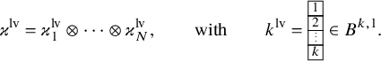
We observe that $\varkappa ^{\mathrm {lv}}$
is the unique element of the crystal
$\varkappa ^{\mathrm {lv}}$
is the unique element of the crystal $B^\varkappa $
with content equal to
$B^\varkappa $
with content equal to $\varkappa ^+$
.
$\varkappa ^+$
.
An immediate consequence of connectedness of affine crystal graphs is that, if two affine crystals $\widehat {B}(\varkappa ),\widehat {B}(\eta )$
are isomorphic, then such isomorphism
$\widehat {B}(\varkappa ),\widehat {B}(\eta )$
are isomorphic, then such isomorphism $\phi $
is unique and moreover
$\phi $
is unique and moreover $\eta ^+=\varkappa ^+$
.
$\eta ^+=\varkappa ^+$
.
Proposition 5.5. For two compositions $\varkappa $
and
$\varkappa $
and $\eta $
, let
$\eta $
, let $\phi :B^\varkappa \to B^\eta $
be an isomorphism between the crystal graphs,
$\phi :B^\varkappa \to B^\eta $
be an isomorphism between the crystal graphs, $B^\varkappa $
and
$B^\varkappa $
and $B^\eta $
. Then
$B^\eta $
. Then $\phi $
is unique and can be expressed as
$\phi $
is unique and can be expressed as
 $$ \begin{align} \phi(b) = h_b^{-1}( \eta^{\mathrm{lv}} ), \end{align} $$
where $h_b$
is any composition of Kashiwara operators such that
$h_b$
is any composition of Kashiwara operators such that $h_b:b \mapsto \varkappa ^{\mathrm {lv}}$
.
$h_b:b \mapsto \varkappa ^{\mathrm {lv}}$
.
Proof. The image of the leading vector $\varkappa ^{\mathrm {lv}}$
must be
$\varkappa ^{\mathrm {lv}}$
must be $\eta ^{\mathrm {lv}}$
by content considerations, and this uniquely determines
$\eta ^{\mathrm {lv}}$
by content considerations, and this uniquely determines $\phi (b)$
for all
$\phi (b)$
for all $b\in B^\varkappa $
. Let
$b\in B^\varkappa $
. Let $b'=\phi (b)$
and consider a map
$b'=\phi (b)$
and consider a map $h_b$
. Since
$h_b$
. Since $\phi $
is a morphism, we have
$\phi $
is a morphism, we have
 $$ \begin{align} b' = \phi(b) = h_b^{-1} \circ h_b \circ \phi(b) = h_b^{-1} \circ \phi \circ h_b(b) = h_b^{-1} \circ \phi ( \varkappa^{\mathrm{lv}} ) = h_b^{-1}( \eta^{\mathrm{lv}} ). \end{align} $$
This proves the proposition.
5.4 Pairs of tableaux as affine bicrystals
In this subsection, we present a novel realization of an affine bicrystal structure on the set of pairs of (generalized) semistandard Young tableaux. Let us define the action of two families of Kashiwara operators $\widetilde {E}_i^{(\epsilon )}, \widetilde {F}_i^{(\epsilon )}$
,
$\widetilde {E}_i^{(\epsilon )}, \widetilde {F}_i^{(\epsilon )}$
, $\epsilon =1,2$
on a pair of semistandard Young tableaux
$\epsilon =1,2$
on a pair of semistandard Young tableaux $(P,Q)$
as follows. For
$(P,Q)$
as follows. For $i=1,\dots , n-1$
, they are given by equation (5.1), whereas for
$i=1,\dots , n-1$
, they are given by equation (5.1), whereas for $i=0$
we set
$i=0$
we set
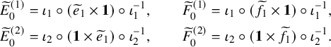 $$ \begin{align} \begin{aligned} &\widetilde{E}_0^{(1)} = \iota_1 \circ ( \widetilde{e}_{1} \times \mathbf{1} ) \circ \iota_1^{-1}, \qquad \widetilde{F}_0^{(1)} = \iota_1 \circ ( \widetilde{f}_{1} \times \mathbf{1} ) \circ \iota_1^{-1}, \\ &\widetilde{E}_0^{(2)} = \iota_2 \circ ( \mathbf{1} \times \widetilde{e}_{1} ) \circ \iota_2^{-1}, \qquad \widetilde{F}_0^{(2)} = \iota_2 \circ ( \mathbf{1} \times \widetilde{f}_{1} ) \circ \iota_2^{-1} . \end{aligned} \end{align} $$
Compare equation (5.13) with equation (5.7). Below in Corollary 5.9 we will show a consistency of these under the projection $\Phi $
(4.21).
$\Phi $
(4.21).
Proposition 5.6. The two families of Kashiwara operators defined above equip the set
 $$ \begin{align} \bigcup_{\rho , \lambda} SST( \lambda / \rho , n ) \times SST( \lambda / \rho , n ) \end{align} $$
with an $\widehat {\mathfrak {sl}}_n$
bicrystal structure.
$\widehat {\mathfrak {sl}}_n$
bicrystal structure.
Proof. It is straightforward to verify that each of the families $\widetilde {E}^{(\epsilon )}_i,\widetilde {F}^{(\epsilon )}_i$
satisfy the hypothesis listed in Section 5.1 so that they both endow the set of pairs
$\widetilde {E}^{(\epsilon )}_i,\widetilde {F}^{(\epsilon )}_i$
satisfy the hypothesis listed in Section 5.1 so that they both endow the set of pairs $(P,Q)$
of an affine crystal structure. It remains to show that these two families are commuting. Clearly, for all
$(P,Q)$
of an affine crystal structure. It remains to show that these two families are commuting. Clearly, for all $i,j=1,\dots ,n-1$
, we have
$i,j=1,\dots ,n-1$
, we have
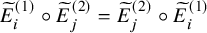 $$ \begin{align} \widetilde{E}^{(1)}_i \circ \widetilde{E}^{(2)}_j = \widetilde{E}^{(2)}_j \circ \widetilde{E}^{(1)}_i \end{align} $$
and similarly for other relations involving also $\widetilde {F}^{(1)}_i, \widetilde {F}^{(2)}_j$
. Let us now show that equation (5.15) holds for
$\widetilde {F}^{(1)}_i, \widetilde {F}^{(2)}_j$
. Let us now show that equation (5.15) holds for $j=0$
and
$j=0$
and $i=0,1,\dots ,n-1$
. Following Proposition 3.24,
$i=0,1,\dots ,n-1$
. Following Proposition 3.24, $\iota _1,\iota _2$
commute, so we need to show that
$\iota _1,\iota _2$
commute, so we need to show that $\iota _2$
commutes with
$\iota _2$
commutes with $\widetilde {E}^{(1)}_i$
for
$\widetilde {E}^{(1)}_i$
for $i=1,\dots ,n-1$
. This last statement is a consequence of Proposition 5.3 yielding the proof.
$i=1,\dots ,n-1$
. This last statement is a consequence of Proposition 5.3 yielding the proof.
The following theorem gives a characterization of symmetries of the skew $\mathbf {RSK}$
map.
$\mathbf {RSK}$
map.
Theorem 5.7. The skew $\mathbf {RSK}$
map is an isomorphism of
$\mathbf {RSK}$
map is an isomorphism of $\widehat {\mathfrak {sl}}_n$
bicrystals.
$\widehat {\mathfrak {sl}}_n$
bicrystals.
Proof. The skew $\mathbf {RSK}$
map clearly commutes with
$\mathbf {RSK}$
map clearly commutes with $\iota _1,\iota _2$
as a result of Proposition 3.6. If
$\iota _1,\iota _2$
as a result of Proposition 3.6. If $P,Q\in SST(\lambda / \rho ,n)$
and
$P,Q\in SST(\lambda / \rho ,n)$
and $(P',Q')=\mathbf {RSK}(P,Q)$
, again by Proposition 3.6,
$(P',Q')=\mathbf {RSK}(P,Q)$
, again by Proposition 3.6, $P',Q'$
are obtained, respectively, from
$P',Q'$
are obtained, respectively, from $P,Q$
after a sequence of internal insertions. By Proposition 5.3, this implies that the skew
$P,Q$
after a sequence of internal insertions. By Proposition 5.3, this implies that the skew $\mathbf {RSK}$
map commutes with classical operators
$\mathbf {RSK}$
map commutes with classical operators $\widetilde {E}^{(\epsilon )}_i, \widetilde {F}^{(\epsilon )}_i$
for
$\widetilde {E}^{(\epsilon )}_i, \widetilde {F}^{(\epsilon )}_i$
for $i=1,\dots ,n-1$
,
$i=1,\dots ,n-1$
, $\epsilon =1,2$
. This shows that
$\epsilon =1,2$
. This shows that $\mathbf {RSK}$
is a morphism of bicrystals. Analogously, one can show that the inverse
$\mathbf {RSK}$
is a morphism of bicrystals. Analogously, one can show that the inverse $\mathbf {RSK}^{-1}$
, which is always defined, is a morphism of bicrystals, concluding the proof.
$\mathbf {RSK}^{-1}$
, which is always defined, is a morphism of bicrystals, concluding the proof.
In the example reported in Figure 14, the statement of Proposition 5.7 is expressed in the form of a commutative diagram that the reader can easily check.
The skew $\mathbf {RSK}$
map commutes with the two families of Kashiwara operators
$\mathbf {RSK}$
map commutes with the two families of Kashiwara operators $\widetilde {E}^{(\epsilon )}_i, \widetilde {F}^{(\epsilon )}_i, i=0,\dots ,n-1$
,
$\widetilde {E}^{(\epsilon )}_i, \widetilde {F}^{(\epsilon )}_i, i=0,\dots ,n-1$
, $\epsilon =1,2$
.
$\epsilon =1,2$
.
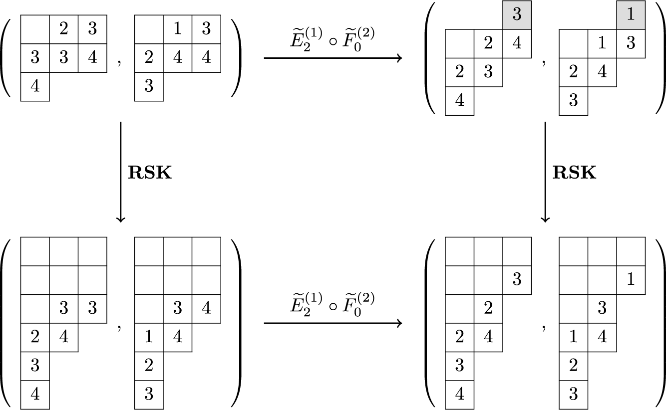
Remark 5.8. We will show in Section 7.5 that, modulo symmetries prescribed by Proposition 5.7, the skew $\mathbf {RSK}$
map is in fact a linear transformation. This implies that the affine bicrystal structure completely characterizes the skew
$\mathbf {RSK}$
map is in fact a linear transformation. This implies that the affine bicrystal structure completely characterizes the skew $\mathbf {RSK}$
map and hence the Sagan–Stanley correspondence of Proposition 4.11.
$\mathbf {RSK}$
map and hence the Sagan–Stanley correspondence of Proposition 4.11.
Corollary 5.9. The projection $\Phi :(P,Q) \mapsto (V,W)$
defined by equation (4.21) is a morphism of affine crystal graphs.
$\Phi :(P,Q) \mapsto (V,W)$
defined by equation (4.21) is a morphism of affine crystal graphs.
Proof. Composition of morphisms of crystals is clearly a morphism of crystals and so is $\mathbf {RSK}^t$
for any t. This implies that
$\mathbf {RSK}^t$
for any t. This implies that $\widetilde {E}^{(\epsilon )}_i \circ \mathbf {RSK}^t(P,Q) = \mathbf {RSK}^t \circ \widetilde {E}^{(\epsilon )}_i (P,Q)$
and hence
$\widetilde {E}^{(\epsilon )}_i \circ \mathbf {RSK}^t(P,Q) = \mathbf {RSK}^t \circ \widetilde {E}^{(\epsilon )}_i (P,Q)$
and hence
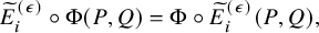 $$ \begin{align} \widetilde{E}^{(\epsilon)}_i \circ \Phi (P,Q) = \Phi \circ \widetilde{E}^{(\epsilon)}_i(P,Q), \end{align} $$
for all $i=1,\dots ,n-1$
,
$i=1,\dots ,n-1$
, $\epsilon =1,2$
since classical operators
$\epsilon =1,2$
since classical operators $\widetilde {E}^{(\epsilon )}_i$
are defined in the same way for semistandard tableaux and vertically strict tableaux. To prove that equation (5.16) holds also for
$\widetilde {E}^{(\epsilon )}_i$
are defined in the same way for semistandard tableaux and vertically strict tableaux. To prove that equation (5.16) holds also for $i=0$
, we compare the action of
$i=0$
, we compare the action of $\iota _1,\iota _2$
and the promotion operator. We call
$\iota _1,\iota _2$
and the promotion operator. We call $(P_t,Q_t)=\mathbf {RSK}^{t-1}(P,Q)$
, and
$(P_t,Q_t)=\mathbf {RSK}^{t-1}(P,Q)$
, and $(\tilde {P}_t,\tilde {Q}_t)=\iota _2^{-1}(P_t,Q_t)$
. Also, denote by
$(\tilde {P}_t,\tilde {Q}_t)=\iota _2^{-1}(P_t,Q_t)$
. Also, denote by $\mu $
the asymptotic increment of
$\mu $
the asymptotic increment of $(P,Q)$
. Then, when t is very large, say large enough so that
$(P,Q)$
. Then, when t is very large, say large enough so that $(P_{t-1},Q_{t-1})$
is
$(P_{t-1},Q_{t-1})$
is $\mathbf {RSK}$
-stable, we see that
$\mathbf {RSK}$
-stable, we see that
-
1. The contents at column j of
$P_t$
and
$\tilde {P}_t$
are equal; -
2. Defining
$b_j,\tilde {b}_j \in B^{\mu _j^{\prime },1}$
as j-th columns respectively of
$Q_t,\tilde {Q}_t$
, we have
$\tilde {b}_j = \mathrm {pr} (b_j)$
, for all
$j=1,2,\dots $
. This is because during inverse internal insertion with cycling
$\iota _2^{-1}$
, i-cells of
$Q_t$
become
$(i+1)$
-cells of
$\tilde {Q}_t$
for
$i=1,\dots ,n-1$
, while n-cells of
$Q_t$
are vacated and new
$1$
-cells are created at the same column as a result of
$\mathbf {RSK}$
-stability. This operation is nothing but promotion on individual columns; see Section 5.3.


Therefore, assuming $\Phi (P,Q)=(V,W)$
, we have
$\Phi (P,Q)=(V,W)$
, we have $\Phi \circ \iota _2^{-1}(P,Q) = (V,\mathrm {pr} (W))$
and by a similar argument
$\Phi \circ \iota _2^{-1}(P,Q) = (V,\mathrm {pr} (W))$
and by a similar argument $\Phi \circ \iota _1^{-1}(P,Q) = (\mathrm {pr} (V), W)$
. Comparing the definition of the 0-th Kashiwara operators for pairs of semistandard tableaux and vertically strict tableaux, we can now conclude that equation (5.16) holds also for
$\Phi \circ \iota _1^{-1}(P,Q) = (\mathrm {pr} (V), W)$
. Comparing the definition of the 0-th Kashiwara operators for pairs of semistandard tableaux and vertically strict tableaux, we can now conclude that equation (5.16) holds also for $i=0$
and
$i=0$
and $\Phi $
is a morphism of
$\Phi $
is a morphism of $\widehat {\mathfrak {sl}}_n$
bicrystals.
$\widehat {\mathfrak {sl}}_n$
bicrystals.
The result of Proposition 5.9 establishes consistency between the bicrystal structure for pairs of vertically strict tableaux and that of pairs of semistandard tableaux. This consideration justifies the following definition.
Definition 5.10. Let $(V,W) = \Phi (P,Q)$
and consider an operator
$(V,W) = \Phi (P,Q)$
and consider an operator
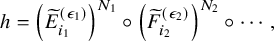 $$ \begin{align} h=\left( \widetilde{E}^{(\epsilon_1)}_{i_1}\right)^{N_1} \circ \left(\widetilde{F}^{(\epsilon_2)}_{i_2}\right)^{N_2} \circ \cdots, \end{align} $$
that is an arbitrary composition of Kashiwara operators such that $h(V,W) \neq \varnothing $
. Then the action of the operator h is defined also on the pair
$h(V,W) \neq \varnothing $
. Then the action of the operator h is defined also on the pair $(P,Q)$
, replacing Kashiwara operators for vertically strict tableaux by the corresponding operators for skew tableaux. Under these assumptions,
$(P,Q)$
, replacing Kashiwara operators for vertically strict tableaux by the corresponding operators for skew tableaux. Under these assumptions, $h(P,Q) \neq \varnothing $
and we call such map the
$h(P,Q) \neq \varnothing $
and we call such map the $\Phi $
-pullback of h. For simplicity, we will not introduce a special notation to denote pullback maps.
$\Phi $
-pullback of h. For simplicity, we will not introduce a special notation to denote pullback maps.
Remark 5.11. The $\widehat {\mathfrak {sl}}_n$
bicrystal structure on the set of pairs
$\widehat {\mathfrak {sl}}_n$
bicrystal structure on the set of pairs $(P,Q)$
defines an
$(P,Q)$
defines an $\widehat {\mathfrak {sl}}_n$
crystal structure on the set of single semistandard Young tableaux of generalized shape. This is done defining Kashiwara operators
$\widehat {\mathfrak {sl}}_n$
crystal structure on the set of single semistandard Young tableaux of generalized shape. This is done defining Kashiwara operators $\widetilde {E}_i(P) = P'$
, if
$\widetilde {E}_i(P) = P'$
, if $\widetilde {E}_i^{(1)} \circ \widetilde {E}_i^{(2)} (P,P) = (P',P')$
. This yields an affine crystal structure different than the one described in [Reference Shimozono80], whose 0-th operators were given by equation (5.7), where
$\widetilde {E}_i^{(1)} \circ \widetilde {E}_i^{(2)} (P,P) = (P',P')$
. This yields an affine crystal structure different than the one described in [Reference Shimozono80], whose 0-th operators were given by equation (5.7), where $\mathrm {pr}$
becomes the Lascoux-Schützenberger promotion operator. For instance, we can check that
$\mathrm {pr}$
becomes the Lascoux-Schützenberger promotion operator. For instance, we can check that
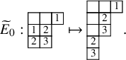
In general, it is not simple to describe concretely the effect of the action of $0$
-th Kashiwara operators on the shape of skew tableaux
$0$
-th Kashiwara operators on the shape of skew tableaux $(P,Q)$
. The next proposition does this in the case of pairs that are
$(P,Q)$
. The next proposition does this in the case of pairs that are $\mathbf {RSK}$
-stable.
$\mathbf {RSK}$
-stable.
Proposition 5.12. Let $P,Q \in SST(\lambda /\rho ,n)$
such that
$P,Q \in SST(\lambda /\rho ,n)$
such that $\iota _1^{-1}(P,Q)$
is an
$\iota _1^{-1}(P,Q)$
is an $\mathbf {RSK}$
-stable pair of tableaux. Define also
$\mathbf {RSK}$
-stable pair of tableaux. Define also $\Phi (P,Q)=(V,W)$
. Identify V with the tensor product of its columns
$\Phi (P,Q)=(V,W)$
. Identify V with the tensor product of its columns $v_1 \otimes \cdots \otimes v_N$
and assume that
$v_1 \otimes \cdots \otimes v_N$
and assume that
 $$ \begin{align} \widetilde{f}_{0}(V) = v_1 \otimes \cdots \otimes \widetilde{f}_{0}(v_k) \otimes \cdots \otimes v_N, \end{align} $$
for some k. Define $(\widetilde {P},\widetilde {Q})=\widetilde {F}_0^{(1)}(P,Q)$
and let
$(\widetilde {P},\widetilde {Q})=\widetilde {F}_0^{(1)}(P,Q)$
and let $\widetilde {\lambda } / \widetilde {\rho }$
be the shape of
$\widetilde {\lambda } / \widetilde {\rho }$
be the shape of $\widetilde {P},\widetilde {Q}$
. Then
$\widetilde {P},\widetilde {Q}$
. Then
 $$ \begin{align} \widetilde{\lambda}^{\prime}_j = \lambda^{\prime}_j + \mathbf{1}_{j=k} \qquad \text{and} \qquad \widetilde{\rho}^{\prime}_j = \rho^{\prime}_j + \mathbf{1}_{j=k}. \end{align} $$
Relations (5.20) hold also for the action of $\widetilde {F}_0^{(2)}$
if we assume that
$\widetilde {F}_0^{(2)}$
if we assume that $(\widetilde {P},\widetilde {Q})=\widetilde {F}_0^{(2)}(P,Q)$
,
$(\widetilde {P},\widetilde {Q})=\widetilde {F}_0^{(2)}(P,Q)$
, $\widetilde {f}_0(W) = w_1\otimes \cdots \otimes \widetilde {f}_0(w_k) \otimes \cdots \otimes w_N$
, where
$\widetilde {f}_0(W) = w_1\otimes \cdots \otimes \widetilde {f}_0(w_k) \otimes \cdots \otimes w_N$
, where $w_i$
’s are columns of W. For the action of inverse operators
$w_i$
’s are columns of W. For the action of inverse operators $\widetilde {E}^{(1)}_0, \widetilde {E}^{(2)}_0$
relations (5.20) hold replacing
$\widetilde {E}^{(1)}_0, \widetilde {E}^{(2)}_0$
relations (5.20) hold replacing $\mathbf {1}_{j=k}$
by
$\mathbf {1}_{j=k}$
by $-\mathbf {1}_{j=k}$
if we assume that
$-\mathbf {1}_{j=k}$
if we assume that $\widetilde {e}_{0}(V) = v_1 \otimes \cdots \otimes \widetilde {e}_{0}(v_k) \otimes \cdots \otimes v_N$
.
$\widetilde {e}_{0}(V) = v_1 \otimes \cdots \otimes \widetilde {e}_{0}(v_k) \otimes \cdots \otimes v_N$
.
Proof. Let $(\widehat {P},\widehat {Q})=\iota _1^{-1}(P,Q)$
, and call
$(\widehat {P},\widehat {Q})=\iota _1^{-1}(P,Q)$
, and call $\widehat {\lambda }/ \widehat {\rho }$
the shape of the pair. Define
$\widehat {\lambda }/ \widehat {\rho }$
the shape of the pair. Define $\theta ^{(i)}(P)=(\theta _1^{(i)} (P),\dots ,\theta _{\lambda _1}^{(i)} (P))$
as
$\theta ^{(i)}(P)=(\theta _1^{(i)} (P),\dots ,\theta _{\lambda _1}^{(i)} (P))$
as
 $$ \begin{align} \theta_c^{(i)}(P) = \mathbf{1}_{\{ \textrm{there is an } i\textrm{-cell at column } c \textrm{ of } P \} }. \end{align} $$
Then, by definition of $\iota _1^{-1}$
and by the property of
$\iota _1^{-1}$
and by the property of $\mathbf {RSK}$
-stability of
$\mathbf {RSK}$
-stability of $(\widehat {P},\widehat {Q})$
, we have
$(\widehat {P},\widehat {Q})$
, we have
 $$ \begin{align} \widehat{\lambda}'=\lambda' - \theta^{(n)}(P) \qquad \text{and} \qquad \widehat{\rho}'=\rho' - \theta^{(n)}(P). \end{align} $$
Clearly, if $(\widehat {P},\widehat {Q})$
is
$(\widehat {P},\widehat {Q})$
is $\mathbf {RSK}$
-stable so is
$\mathbf {RSK}$
-stable so is $(\widetilde {f}_{j}(\widehat {P}),\widehat {Q})$
whenever
$(\widetilde {f}_{j}(\widehat {P}),\widehat {Q})$
whenever $j=1,\dots ,n-1$
and
$j=1,\dots ,n-1$
and $\widetilde {f}_{j}(\widehat {P})\neq \varnothing $
. Then as above we have
$\widetilde {f}_{j}(\widehat {P})\neq \varnothing $
. Then as above we have
 $$ \begin{align} \widetilde{\lambda}' = \widehat{\lambda}' + \theta^{(1)}(\widetilde{f}_{1}(\widehat{P})) = \lambda' - \theta^{(n)}(P) + \theta^{(1)}(\widetilde{f}_{i}(\widehat{P})) \end{align} $$
and similarly for $\widetilde {\rho }$
, which is exactly the claim (5.20). The proof of relations (5.20) for the action of operators
$\widetilde {\rho }$
, which is exactly the claim (5.20). The proof of relations (5.20) for the action of operators $\widetilde {F}_0^{(2)}, \widetilde {E}_0^{(1)}, \widetilde {E}_0^{(2)}$
is analogous and therefore is omitted.
$\widetilde {F}_0^{(2)}, \widetilde {E}_0^{(1)}, \widetilde {E}_0^{(2)}$
is analogous and therefore is omitted.
5.5 Matrices
$\overline {\mathbb {M}}_{n\times n}$
as affine bicrystals

We equip the set of matrices $\overline {\mathbb {M}}_{n\times n}$
of an
$\overline {\mathbb {M}}_{n\times n}$
of an $\widehat {\mathfrak {sl}}_n$
bicrystal structure, transporting, via the Sagan–Stanley correspondence, the structure on the set of pairs of tableaux discussed in Section 5.4. Similar investigations were recently pursued in [Reference Gerber and Lecouvey35], where authors considered the set of infinite binary matrices as affine bicrystals. For the case of integral matrices
$\widehat {\mathfrak {sl}}_n$
bicrystal structure, transporting, via the Sagan–Stanley correspondence, the structure on the set of pairs of tableaux discussed in Section 5.4. Similar investigations were recently pursued in [Reference Gerber and Lecouvey35], where authors considered the set of infinite binary matrices as affine bicrystals. For the case of integral matrices $\mathbb {M}_{n\times n}$
classical bicrystal structure had been discussed in [Reference Danilov and Koshevoy23, Reference van Leeuwen86].
$\mathbb {M}_{n\times n}$
classical bicrystal structure had been discussed in [Reference Danilov and Koshevoy23, Reference van Leeuwen86].
We start defining the action of two families of classical Kashiwara operators on the set of matrices $\overline {\mathbb {M}}_{n\times n}$
. For a given
$\overline {\mathbb {M}}_{n\times n}$
. For a given $\overline {M}\in \overline {\mathbb {M}}_{n \times n}$
and
$\overline {M}\in \overline {\mathbb {M}}_{n \times n}$
and $i=1,\dots ,n-1$
, we set
$i=1,\dots ,n-1$
, we set
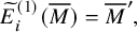 $$ \begin{align} \widetilde{E}_i^{(1)} ( \overline{M} ) = \overline{M}', \end{align} $$
where $\overline {M}'$
, as a map on
$\overline {M}'$
, as a map on $\mathscr {C}_n$
, is
$\mathscr {C}_n$
, is
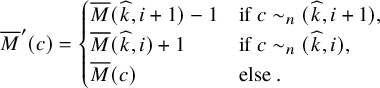 $$ \begin{align} \overline{M}' (c) = \begin{cases} \overline{M} (\widehat{k} , i+1) - 1 \qquad & \text{if } c \sim_n (\widehat{k},i+1), \\ \overline{M} (\widehat{k} , i) + 1 \qquad & \text{if } c \sim_n (\widehat{k},i), \\ \overline{M} (c) \qquad & \text{else }. \end{cases} \end{align} $$
The value of $\widehat {k}$
is determined by the signature rule, that in this case reads
$\widehat {k}$
is determined by the signature rule, that in this case reads
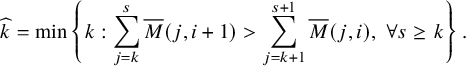 $$ \begin{align} \widehat{k} = \min \left\{ k : \sum_{j = k}^{s} \overline{M} (j,i+1)> \sum_{j = k+1}^{s+1} \overline{M} (j,i), \,\, \forall s \ge k \right\}. \end{align} $$
See Figure 15 for an example.


Analogously, we define $\widetilde {F}^{(1)}_i$
as the (partial) inverse of
$\widetilde {F}^{(1)}_i$
as the (partial) inverse of $\widetilde {E}^{(1)}_i$
, that is,
$\widetilde {E}^{(1)}_i$
, that is,
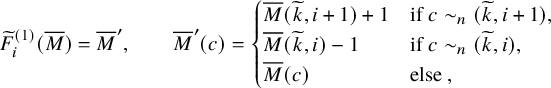 $$ \begin{align} \widetilde{F}_i^{(1)} ( \overline{M} ) = \overline{M}', \qquad \overline{M}' (c) = \begin{cases} \overline{M} (\widetilde{k} , i+1) + 1 \qquad & \text{if } c \sim_n (\widetilde{k},i+1), \\ \overline{M} (\widetilde{k} , i) - 1 \qquad & \text{if } c \sim_n (\widetilde{k},i), \\ \overline{M} (c) \qquad & \text{else }, \end{cases} \end{align} $$
where this time
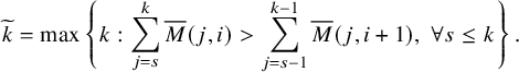 $$ \begin{align} \widetilde{k} = \max \left\{ k : \sum_{j =s}^k \overline{M} (j,i)> \sum_{j = s-1}^{k-1} \overline{M} (j,i+1), \,\, \forall s \le k \right\}. \end{align} $$
In order to define the $0$
-th Kashiwara operators, we introduce the shifts
$0$
-th Kashiwara operators, we introduce the shifts
 $$ \begin{align} T_{\epsilon}(f)(c) = f(c-\mathbf{e}_{\epsilon}), \end{align} $$
for $\epsilon =1,2$
, acting on any map f from the twisted cylinder
$\epsilon =1,2$
, acting on any map f from the twisted cylinder $\mathscr {C}_n$
. We set
$\mathscr {C}_n$
. We set
 $$ \begin{align} \widetilde{E}^{(1)}_0 = T_2 \circ \widetilde{E}^{(1)}_1 \circ T_2^{-1}, \qquad \widetilde{F}^{(1)}_0 = T_2 \circ \widetilde{F}^{(1)}_1 \circ T_2^{-1}. \end{align} $$
The second family of Kashiwara operators is defined by duality,
 $$ \begin{align} \widetilde{E}^{(2)}_i(\overline{M}^T) = \widetilde{E}^{(1)}_i(\overline{M})^T, \qquad \widetilde{F}^{(2)}_i(\overline{M}^T) = \widetilde{F}^{(1)}_i(\overline{M})^T. \end{align} $$
Remark 5.13. We can translate the definitions for matrices above to those for weighted biwords through identification (2.6). For instance, classical Kashiwara operators become
and analogously for the $\widetilde {F}^{(1)}_i$
operator for
$\widetilde {F}^{(1)}_i$
operator for $i=1,\dots , n-1$
. Notice that defining the signature rule on matrices
$i=1,\dots , n-1$
. Notice that defining the signature rule on matrices $\overline {M}$
concatenating slices
$\overline {M}$
concatenating slices $\overline {M}(k)$
’s in decreasing order in k results in the appearance of the timetable ordering of
$\overline {M}(k)$
’s in decreasing order in k results in the appearance of the timetable ordering of
![]() in the language of weighted biwords; see Figure 15. The second family
in the language of weighted biwords; see Figure 15. The second family $\widetilde {E}^{(2)}_i,\widetilde {F}^{(2)}_i$
, again for
$\widetilde {E}^{(2)}_i,\widetilde {F}^{(2)}_i$
, again for $i=1,\dots ,n-1$
, is defined by duality
$i=1,\dots ,n-1$
, is defined by duality
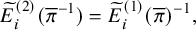 $$ \begin{align} \widetilde{E}^{(2)}_i (\overline{\pi}^{-1}) = \widetilde{E}^{(1)}_i (\overline{\pi})^{-1}, \end{align} $$
and similarly for the $F^{(2)}_i$
operators.
$F^{(2)}_i$
operators.
Proposition 5.14. The two families $\{\widetilde {E}^{(\epsilon )}_i, \widetilde {F}^{(\epsilon )}_i : i=0,\dots ,n-1 \}$
,
$\{\widetilde {E}^{(\epsilon )}_i, \widetilde {F}^{(\epsilon )}_i : i=0,\dots ,n-1 \}$
, $\epsilon =1,2$
defined above equip the set
$\epsilon =1,2$
defined above equip the set $\overline {\mathbb {M}}_{n \times n}$
of an
$\overline {\mathbb {M}}_{n \times n}$
of an $\widehat {\mathfrak {sl}}_n$
bicrystal structure.
$\widehat {\mathfrak {sl}}_n$
bicrystal structure.
Proof. Defining the content functions $\gamma ^{(1)},\gamma ^{(2)}$
as
$\gamma ^{(1)},\gamma ^{(2)}$
as
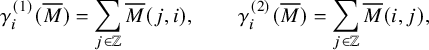 $$ \begin{align} \gamma^{(1)}_i (\overline{M}) = \sum_{j\in \mathbb{Z}} \overline{M}(j,i), \qquad \gamma^{(2)}_i (\overline{M}) = \sum_{j\in \mathbb{Z}} \overline{M}(i,j), \end{align} $$
it is straightforward to verify that $\widetilde {E}^{(1)}_i, \widetilde {F}^{(1)}_i$
and
$\widetilde {E}^{(1)}_i, \widetilde {F}^{(1)}_i$
and $\widetilde {E}^{(2)}_i, \widetilde {F}^{(2)}_i$
fulfill hypothesis enumerated in Section 5.1. Commutativity of the two families of Kashiwara operators can also be checked directly. This was done for finite integral matrices in [Reference Danilov and Koshevoy23, Reference van Leeuwen86].
$\widetilde {E}^{(2)}_i, \widetilde {F}^{(2)}_i$
fulfill hypothesis enumerated in Section 5.1. Commutativity of the two families of Kashiwara operators can also be checked directly. This was done for finite integral matrices in [Reference Danilov and Koshevoy23, Reference van Leeuwen86].
The affine bicrystal structure we impose on the set of matrices $\overline {\mathbb {M}}_{n \times n}$
is by design compatible with the bicrystal structure defined on set of pairs of tableaux.
$\overline {\mathbb {M}}_{n \times n}$
is by design compatible with the bicrystal structure defined on set of pairs of tableaux.
Proposition 5.15. The map (4.13) $(P,Q) \xrightarrow []{\mathbf {SS}\,} \overline {M}$
is a morphism of
$(P,Q) \xrightarrow []{\mathbf {SS}\,} \overline {M}$
is a morphism of $\widehat {\mathfrak {sl}}_n$
bicrystals.
$\widehat {\mathfrak {sl}}_n$
bicrystals.
Proof. We first show that $(P,Q) \xrightarrow []{\mathbf {SS}\,} \overline {M}$
is a morphism of
$(P,Q) \xrightarrow []{\mathbf {SS}\,} \overline {M}$
is a morphism of $\mathfrak {sl}_n$
bicrystals. For this, it is convenient to use the formalism of weighted biwords
$\mathfrak {sl}_n$
bicrystals. For this, it is convenient to use the formalism of weighted biwords $\overline {\pi }(\overline {M})$
, whose bicrystal structure was given in Proposition 5.13, rather than matrices. If
$\overline {\pi }(\overline {M})$
, whose bicrystal structure was given in Proposition 5.13, rather than matrices. If $(P,Q) \xrightarrow []{\mathbf {SS}\,} \overline {\pi }$
, call
$(P,Q) \xrightarrow []{\mathbf {SS}\,} \overline {\pi }$
, call $\pi _P$
the row reading word of P and
$\pi _P$
the row reading word of P and
![]() . By Proposition A.6, we have
. By Proposition A.6, we have $\pi _P \simeq p$
, where
$\pi _P \simeq p$
, where $\simeq $
denotes the Knuth equivalence. Notice that, the statement in Proposition A.6 requires that tableau P is of classical shape for simplicity, but it is straightforward to understand this assumption is not needed. Since
$\simeq $
denotes the Knuth equivalence. Notice that, the statement in Proposition A.6 requires that tableau P is of classical shape for simplicity, but it is straightforward to understand this assumption is not needed. Since $\pi _P \simeq p$
, the map
$\pi _P \simeq p$
, the map $P \mapsto p$
can be realized as a sequence of jeu de taquin moves, identifying the word p with its antidiagonal strip tableau
$P \mapsto p$
can be realized as a sequence of jeu de taquin moves, identifying the word p with its antidiagonal strip tableau

This implies, by Proposition 5.2 that $\widetilde {e}_{i}(P) \mapsto \widetilde {e}_{i}(p)$
and hence
$\widetilde {e}_{i}(P) \mapsto \widetilde {e}_{i}(p)$
and hence
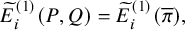 $$ \begin{align} \widetilde{E}_i^{(1)}(P,Q) = \widetilde{E}_i^{(1)}(\overline{\pi}), \end{align} $$
for $i=1,\dots ,n-1$
. The same can be said for the family
$i=1,\dots ,n-1$
. The same can be said for the family $\widetilde {E}_i^{(2)},\widetilde {F}_i^{(1)},\widetilde {F}_i^{(2)}, i=1,\dots ,n-1$
and hence
$\widetilde {E}_i^{(2)},\widetilde {F}_i^{(1)},\widetilde {F}_i^{(2)}, i=1,\dots ,n-1$
and hence $(P,Q) \xrightarrow []{\mathbf {SS}\,} \overline {\pi }$
is a morphism of
$(P,Q) \xrightarrow []{\mathbf {SS}\,} \overline {\pi }$
is a morphism of $\mathfrak {sl}_n$
bicrystals and so is equation (4.13). To prove that
$\mathfrak {sl}_n$
bicrystals and so is equation (4.13). To prove that $(P,Q) \xrightarrow []{\mathbf {SS}\,} \overline {M}$
is a morphism of affine bicrystals, we use Proposition 4.4, which along with Proposition 4.9 implies that
$(P,Q) \xrightarrow []{\mathbf {SS}\,} \overline {M}$
is a morphism of affine bicrystals, we use Proposition 4.4, which along with Proposition 4.9 implies that $\iota _1(P,Q) \xrightarrow []{\mathbf {SS}\,} T_2 (\overline {M}), \iota _2(P,Q) \xrightarrow []{\mathbf {SS}\,} T_1 (\overline {M})$
. This proves that for both
$\iota _1(P,Q) \xrightarrow []{\mathbf {SS}\,} T_2 (\overline {M}), \iota _2(P,Q) \xrightarrow []{\mathbf {SS}\,} T_1 (\overline {M})$
. This proves that for both $\epsilon =1,2$
,
$\epsilon =1,2$
, $\widetilde {E}^{(\epsilon )}_i(P,Q) \mapsto \widetilde {E}^{(\epsilon )}_i(\overline {M})$
,
$\widetilde {E}^{(\epsilon )}_i(P,Q) \mapsto \widetilde {E}^{(\epsilon )}_i(\overline {M})$
, $\widetilde {F}^{(\epsilon )}_i(P,Q) \mapsto \widetilde {F}^{(\epsilon )}_i(\overline {M})$
also for
$\widetilde {F}^{(\epsilon )}_i(P,Q) \mapsto \widetilde {F}^{(\epsilon )}_i(\overline {M})$
also for $i=0$
.
$i=0$
.
The Viennot map commutes with the two families of Kashiwara operators $\widetilde {E}^{(\epsilon )}_i, \widetilde {F}^{(\epsilon )}_i, i=0,\dots ,n-1$
,
$\widetilde {E}^{(\epsilon )}_i, \widetilde {F}^{(\epsilon )}_i, i=0,\dots ,n-1$
, $\epsilon =1,2$
.
$\epsilon =1,2$
.
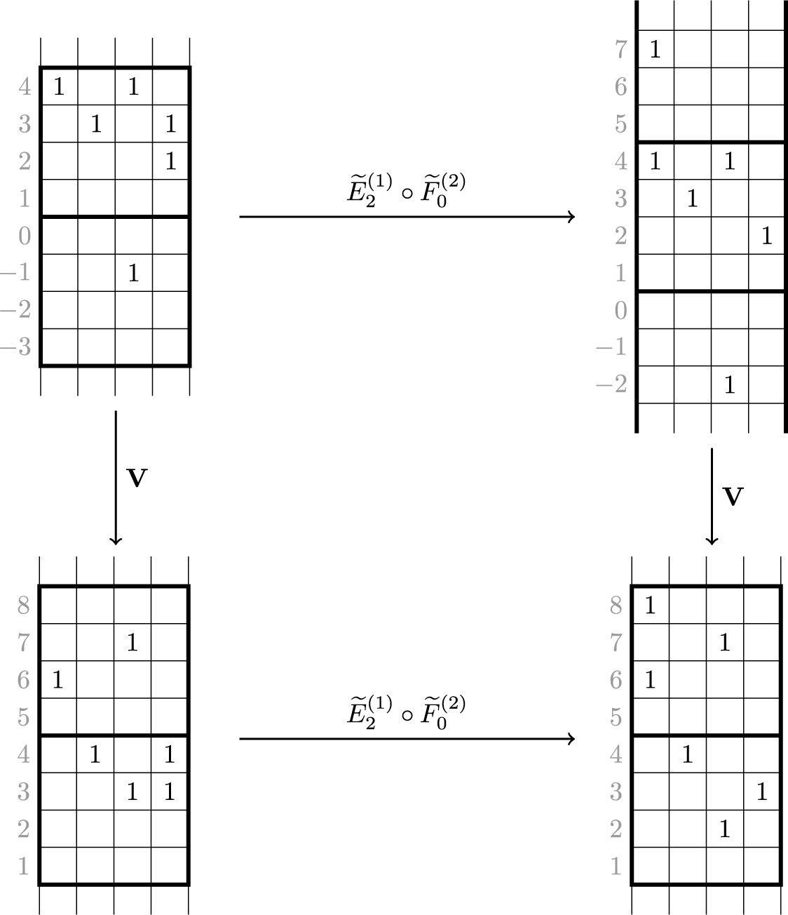
Theorem 5.16. The Viennot map $\mathbf {V}$
is an isomorphism of
$\mathbf {V}$
is an isomorphism of $\widehat {\mathfrak {sl}}_n$
bicrystals.
$\widehat {\mathfrak {sl}}_n$
bicrystals.
Proof. This is a consequence of Proposition 5.15. For any matrix $\overline {M}$
, there always exists a pair of tableaux
$\overline {M}$
, there always exists a pair of tableaux $(P,Q)$
such that
$(P,Q)$
such that $(P,Q) \xrightarrow []{\mathbf {SS} \,} \overline {M}$
under map (4.13). This is a consequence of Proposition 4.9 and of construction reported (only for tableaux of classical shape for brevity) in Proposition 2.3. Let
$(P,Q) \xrightarrow []{\mathbf {SS} \,} \overline {M}$
under map (4.13). This is a consequence of Proposition 4.9 and of construction reported (only for tableaux of classical shape for brevity) in Proposition 2.3. Let $(P',Q')$
be tableaux obtained rigidly shifting
$(P',Q')$
be tableaux obtained rigidly shifting $P,Q$
one row up. Then, by Proposition 4.13 we have
$P,Q$
one row up. Then, by Proposition 4.13 we have $(P',Q') \xrightarrow []{\mathbf {SS} \,} \mathbf {V}(\overline {M})$
. Since the transformation
$(P',Q') \xrightarrow []{\mathbf {SS} \,} \mathbf {V}(\overline {M})$
. Since the transformation $(P,Q) \mapsto (P',Q')$
is realized through a sequence of jeu de taquin moves we have
$(P,Q) \mapsto (P',Q')$
is realized through a sequence of jeu de taquin moves we have $\widetilde {E}^{(\epsilon )}_i(P,Q) \mapsto \widetilde {E}^{(\epsilon )}_i(P',Q')$
and using Proposition 5.15,
$\widetilde {E}^{(\epsilon )}_i(P,Q) \mapsto \widetilde {E}^{(\epsilon )}_i(P',Q')$
and using Proposition 5.15, $\widetilde {E}^{(\epsilon )}_i \circ \mathbf {V}(\overline {M}) = \mathbf {V} \circ \widetilde {E}^{(\epsilon )}_i(\overline {M})$
.
$\widetilde {E}^{(\epsilon )}_i \circ \mathbf {V}(\overline {M}) = \mathbf {V} \circ \widetilde {E}^{(\epsilon )}_i(\overline {M})$
.
In Figure 16, we report an example of commutation relations prescribed by Proposition 5.16.
We could extend the description of crystal operators to matrices of integers $(\alpha , \beta )$
. Such considerations will not play important role in this paper, and therefore we do not discuss them here. The interested reader can consult [Reference Danilov and Koshevoi22], where similar ideas were investigated by the authors.
$(\alpha , \beta )$
. Such considerations will not play important role in this paper, and therefore we do not discuss them here. The interested reader can consult [Reference Danilov and Koshevoi22], where similar ideas were investigated by the authors.
6 Generalized Greene invariants
In this section, we study increasing subsequences and localized decreasing subsequences of weighted biwords or of infinite matrices. These were defined in Section 4.6 and represent generalizations of the classical increasing and decreasing subsequences which in the RSK correspondence capture the shape of the tableaux. We show that the maximal increasing and localized decreasing subsequences are invariant under the action of Kashiwara operators in Proposition 6.4 and that they are preserved by the Viennot map in Proposition 6.5. Their interpretation in the language of tableaux is given in Proposition 6.6, and they describe the asymptotic increment of $(P,Q)$
under skew
$(P,Q)$
under skew $\mathbf {RSK}$
dynamics. From this last fact, we deduce a generalization of Schensted’s theorem describing the first row of the shape of a pair of skew tableaux
$\mathbf {RSK}$
dynamics. From this last fact, we deduce a generalization of Schensted’s theorem describing the first row of the shape of a pair of skew tableaux $(P,Q) \leftrightarrow (\overline {\pi }; \nu )$
in terms of the longest increasing subsequence of
$(P,Q) \leftrightarrow (\overline {\pi }; \nu )$
in terms of the longest increasing subsequence of $\overline {\pi }$
and of
$\overline {\pi }$
and of $\nu _1$
.
$\nu _1$
.
6.1 Passage times and subsequences
In Section 4.6, we defined increasing and localized decreasing subsequences of a weighted biword $\overline {\pi }$
. We now extend these definitions considering decompositions of
$\overline {\pi }$
. We now extend these definitions considering decompositions of $\overline {\pi }$
into multiple subsequences.
$\overline {\pi }$
into multiple subsequences.
Definition 6.1. A weighted biword $\overline {\pi } \in \overline {\mathbb {A}}_{n,n}$
is k-increasing if it can be written as a disjoint union of k increasing weighted biwords
$\overline {\pi } \in \overline {\mathbb {A}}_{n,n}$
is k-increasing if it can be written as a disjoint union of k increasing weighted biwords
![]() . Analogously,
. Analogously, $\overline {\pi }$
is k-localized decreasing if it can be written as a disjoint union of k localized decreasing weighted biwords
$\overline {\pi }$
is k-localized decreasing if it can be written as a disjoint union of k localized decreasing weighted biwords
![]() .
.
Definition 6.2 (Greene invariants).
For a weighted biword $\overline {\pi }\in \overline {\mathbb {A}}_{n,n}$
, we define statistics
$\overline {\pi }\in \overline {\mathbb {A}}_{n,n}$
, we define statistics

If $\overline {M} \in \overline {\mathbb {M}}_{n \times n}$
is the matrix corresponding to
$\overline {M} \in \overline {\mathbb {M}}_{n \times n}$
is the matrix corresponding to $\overline {\pi }$
, we will denote
$\overline {\pi }$
, we will denote $I_k (\overline {M})=I_k (\overline {\pi })$
and the same for
$I_k (\overline {M})=I_k (\overline {\pi })$
and the same for $D_k (\overline {M}) = D_k(\overline {\pi })$
.
$D_k (\overline {M}) = D_k(\overline {\pi })$
.
It is straightforward to notice that the notion of $I_k(\overline {M})$
, defined in Section 1.3 in terms of last passage times of up-right paths is equal to the one given in Proposition 6.2.
$I_k(\overline {M})$
, defined in Section 1.3 in terms of last passage times of up-right paths is equal to the one given in Proposition 6.2.
Remark 6.3. In case $\overline {\pi }$
is such that
$\overline {\pi }$
is such that $w_i(\overline {\pi }) = 0$
for all i notions of increasing and localized decreasing become respectively the usual notions of increasing and decreasing for words [Reference Sagan74, Chapter 3.3].
$w_i(\overline {\pi }) = 0$
for all i notions of increasing and localized decreasing become respectively the usual notions of increasing and decreasing for words [Reference Sagan74, Chapter 3.3].
Statistics $I_k(\overline {\pi }), D_k(\overline {\pi })$
, as we will prove in Proposition 6.4 are invariants under the action of Kashiwara operators. Moreover, in Appendix A.3 we will define a generalized notion of Knuth relations and we will prove in Proposition A.17, that also with respect to these transformations
$I_k(\overline {\pi }), D_k(\overline {\pi })$
, as we will prove in Proposition 6.4 are invariants under the action of Kashiwara operators. Moreover, in Appendix A.3 we will define a generalized notion of Knuth relations and we will prove in Proposition A.17, that also with respect to these transformations $I_k,D_k$
are invariants. Therefore, they represent generalizations in skew setting of Greene invariants, which should justify the terminology used.
$I_k,D_k$
are invariants. Therefore, they represent generalizations in skew setting of Greene invariants, which should justify the terminology used.
6.2 Greene invariants and crystal operators
In classical setting Greene invariants of a biword $\pi $
, or equivalently of an integral matrix M, are known to be invariant under the action of classical Kashiwara operators. This can be proven either using the fact that the RSK algorithm
$\pi $
, or equivalently of an integral matrix M, are known to be invariant under the action of classical Kashiwara operators. This can be proven either using the fact that the RSK algorithm $M \mapsto (P,Q)$
is a morphism of classical crystals and leveraging Greene’s theorem [Reference Bump and Schilling16] or through a direct check [Reference Danilov and Koshevoy23, Reference van Leeuwen86]. In a skew/affine setting, we find that analogous invariances hold, as stated in the next theorem.
$M \mapsto (P,Q)$
is a morphism of classical crystals and leveraging Greene’s theorem [Reference Bump and Schilling16] or through a direct check [Reference Danilov and Koshevoy23, Reference van Leeuwen86]. In a skew/affine setting, we find that analogous invariances hold, as stated in the next theorem.
Theorem 6.4. Let $\overline {\pi } \in \overline {\mathbb {A}}_{n,n}$
. Let
$\overline {\pi } \in \overline {\mathbb {A}}_{n,n}$
. Let $h=\widetilde {E}^{(\epsilon )}_i$
or
$h=\widetilde {E}^{(\epsilon )}_i$
or $h=\widetilde {F}^{(\epsilon )}_i$
for some
$h=\widetilde {F}^{(\epsilon )}_i$
for some $\epsilon =1,2$
,
$\epsilon =1,2$
, $i=0,1,\dots ,n-1$
, and assume
$i=0,1,\dots ,n-1$
, and assume $h(\overline {\pi }) \ne \varnothing $
. Then, for all k, we have
$h(\overline {\pi }) \ne \varnothing $
. Then, for all k, we have
 $$ \begin{align} I_k(h(\overline{\pi})) = I_k(\overline{\pi}) \qquad \text{and} \qquad D_k(h(\overline{\pi})) = D_k(\overline{\pi}). \end{align} $$
Proof of Proposition 6.4 is reported in Appendix B. Arguments we use are rather straightforward and consist in direct checks of conservation laws (6.1). Similar strategies were elaborated in [Reference Danilov and Koshevoy23, Reference van Leeuwen86] in classical setting. Compared to these previous works, our approach is conceptually equivalent, although technically more involved.
6.3 Greene invariants, Viennot map and skew
$\mathbf {RSK}$
dynamics

Here, we describe two main results of this section. The first, given in Proposition 6.5, illustrates fundamental conservation laws of the Viennot map $\mathbf {V}$
. The second, presented in Proposition 6.6, characterizes the asymptotic shape
$\mathbf {V}$
. The second, presented in Proposition 6.6, characterizes the asymptotic shape $\mu (P,Q)$
of a pair of skew tableaux
$\mu (P,Q)$
of a pair of skew tableaux $(P,Q)$
in terms of the Greene invariants
$(P,Q)$
in terms of the Greene invariants $I_k,D_k$
. This second result gives a generalization of Greene’s theorem [Reference Greene36] in skew setting. Proofs of Proposition 6.5 and Proposition 6.6 are reported in Section 6.5 below.
$I_k,D_k$
. This second result gives a generalization of Greene’s theorem [Reference Greene36] in skew setting. Proofs of Proposition 6.5 and Proposition 6.6 are reported in Section 6.5 below.
Theorem 6.5. Let $\overline {\pi } \in \overline {\mathbb {A}}_{n,n}$
. Then for all k we have
$\overline {\pi } \in \overline {\mathbb {A}}_{n,n}$
. Then for all k we have
 $$ \begin{align} I_k(\mathbf{V}(\overline{\pi})) = I_k(\overline{\pi}) \qquad \text{and} \qquad D_k(\mathbf{V}(\overline{\pi})) = D_k(\overline{\pi}). \end{align} $$
For our next statement, associate to each weighted biword $\overline {\pi }$
two a priori different partitions
$\overline {\pi }$
two a priori different partitions $\mu (\overline {\pi })$
and
$\mu (\overline {\pi })$
and $\widetilde {\mu }(\overline {\pi })$
. They are defined through the Greene invariants of
$\widetilde {\mu }(\overline {\pi })$
. They are defined through the Greene invariants of $\overline {\pi }$
as
$\overline {\pi }$
as
 $$ \begin{align} \mu_1^{\prime} + \cdots + \mu_k^{\prime} = D_k(\overline{\pi}), \end{align} $$
 $$ \begin{align} \widetilde{\mu}_1 + \cdots + \widetilde{\mu}_k = I_k(\overline{\pi}). \end{align} $$
Theorem 6.6. Let $P,Q \in SST (\lambda /\rho , n)$
, and consider the projection
$P,Q \in SST (\lambda /\rho , n)$
, and consider the projection $(P,Q) \xrightarrow []{\mathbf {SS} \,} \overline {\pi }$
. Denote by
$(P,Q) \xrightarrow []{\mathbf {SS} \,} \overline {\pi }$
. Denote by $\mu (P,Q)$
the asymptotic increment of
$\mu (P,Q)$
the asymptotic increment of $(P,Q)$
under skew
$(P,Q)$
under skew $\mathbf {RSK}$
dynamics. Then
$\mathbf {RSK}$
dynamics. Then $\mu (P,Q) = \mu (\overline {\pi }) = \widetilde {\mu }(\overline {\pi })$
.
$\mu (P,Q) = \mu (\overline {\pi }) = \widetilde {\mu }(\overline {\pi })$
.
We will see, in Proposition 6.8 below, that establishing invariance of statistics $D_k$
is relatively straightforward and it follows from an intuitive graphical argument. Proving invariance of the length of longest k-increasing subsequences
$D_k$
is relatively straightforward and it follows from an intuitive graphical argument. Proving invariance of the length of longest k-increasing subsequences $I_k$
from the shadow line construction seems to be less elementary. Therefore, we will prove the slightly less direct fact that partitions
$I_k$
from the shadow line construction seems to be less elementary. Therefore, we will prove the slightly less direct fact that partitions $\mu = \widetilde {\mu }$
. For this, we will take advantage of symmetries with respect to crystal operators, provided by Proposition 6.4 and we will also evoke the connectedness property of the affine crystal graph
$\mu = \widetilde {\mu }$
. For this, we will take advantage of symmetries with respect to crystal operators, provided by Proposition 6.4 and we will also evoke the connectedness property of the affine crystal graph $\widehat {B}(\varkappa )$
recalled in Proposition 5.4.
$\widehat {B}(\varkappa )$
recalled in Proposition 5.4.
6.4 An extension of Schensted’s theorem
We present a generalization of Schensted’s theorem [Reference Schensted76]. In a classical setting, this relates the length of the first row of a pair of straight standard tableaux $(P,Q)$
with the longest increasing subsequence of the corresponding permutation
$(P,Q)$
with the longest increasing subsequence of the corresponding permutation $\pi $
.
$\pi $
.
Theorem 6.7. Let $\overline {\pi } \in \overline {\mathbb {A}}_{n,n}^+$
be a weighted biword and
$\overline {\pi } \in \overline {\mathbb {A}}_{n,n}^+$
be a weighted biword and $\nu $
a partition. Let
$\nu $
a partition. Let $\lambda /\rho $
be the skew shape of tableaux
$\lambda /\rho $
be the skew shape of tableaux
![]() . Then
. Then $\lambda _1 = \nu _1 + I_1(\overline {\pi })$
.
$\lambda _1 = \nu _1 + I_1(\overline {\pi })$
.
Proof. This is a simple corollary of Proposition 6.6. By Proposition 3.23, the application of skew $\mathbf {RSK}$
map does not change partition
$\mathbf {RSK}$
map does not change partition $\nu =\ker (P,Q)$
. Let
$\nu =\ker (P,Q)$
. Let
![]() , then if
, then if $(\widetilde {P},\widetilde {Q})=\mathbf {RSK}^t(P,Q)$
and
$(\widetilde {P},\widetilde {Q})=\mathbf {RSK}^t(P,Q)$
and $(\widetilde {\alpha }, \widetilde {\beta })=\mathbf {RSK}^t(\alpha , \beta )$
, we have
$(\widetilde {\alpha }, \widetilde {\beta })=\mathbf {RSK}^t(\alpha , \beta )$
, we have
![]() . When t is large enough the pair
. When t is large enough the pair $(\widetilde {P},\widetilde {Q})$
becomes
$(\widetilde {P},\widetilde {Q})$
becomes $\mathbf {RSK}$
-stable and calling
$\mathbf {RSK}$
-stable and calling $\widetilde {\lambda } / \widetilde {\rho }$
its shape and
$\widetilde {\lambda } / \widetilde {\rho }$
its shape and $\mu $
the asymptotic increment, we have
$\mu $
the asymptotic increment, we have $\widetilde {\lambda }_1 = \nu _1 + \mu _1$
. Since the skew
$\widetilde {\lambda }_1 = \nu _1 + \mu _1$
. Since the skew $\mathbf {RSK}$
map does not modify the length of the first row of tableaux
$\mathbf {RSK}$
map does not modify the length of the first row of tableaux $P,Q$
, we conclude that
$P,Q$
, we conclude that $\lambda _1 = \nu _1+\mu _1$
and hence the claim of the theorem by Proposition 6.6.
$\lambda _1 = \nu _1+\mu _1$
and hence the claim of the theorem by Proposition 6.6.
6.5 Proofs of Proposition 6.5 and of Proposition 6.6
We start by proving that the Viennot map preserves the length of the longest localized decreasing subsequences.
An example of the construction described in the proof of Proposition 6.8. Green circled black bullets correspond to LDS $\overline {\sigma }^{(1)}$
, while blue circled correspond to
$\overline {\sigma }^{(1)}$
, while blue circled correspond to $\overline {\sigma }^{(2)}$
. Red bullets falling on green and blue broken lines determine LDSs
$\overline {\sigma }^{(2)}$
. Red bullets falling on green and blue broken lines determine LDSs $\overline {\xi }^{(1)}$
and
$\overline {\xi }^{(1)}$
and $\overline {\xi }^{(2)}$
of
$\overline {\xi }^{(2)}$
of $\mathbf {V}(\overline {\pi })$
.
$\mathbf {V}(\overline {\pi })$
.
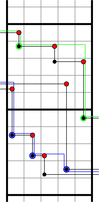
Lemma 6.8. Let $\overline {\pi } \in \overline {\mathbb {A}}_{n,n}$
. Then for all k, we have
$\overline {\pi } \in \overline {\mathbb {A}}_{n,n}$
. Then for all k, we have $D_k(\mathbf {V}(\overline {\pi })) = D_k(\overline {\pi }).$
Proof. Let
![]() be a k-LDS of
be a k-LDS of $\overline {\pi }$
. Consider the shadow line construction of
$\overline {\pi }$
. Consider the shadow line construction of $\overline {\sigma }$
, which by Proposition B.4 consists of at most k down-right loops
$\overline {\sigma }$
, which by Proposition B.4 consists of at most k down-right loops $\overline {\varsigma }^{(1)}, \dots , \overline {\varsigma }^{(k)}$
(note the last few of them could be empty). With no loss of generality we can assume that
$\overline {\varsigma }^{(1)}, \dots , \overline {\varsigma }^{(k)}$
(note the last few of them could be empty). With no loss of generality we can assume that $\overline {\sigma }^{(j)}$
consists of points in
$\overline {\sigma }^{(j)}$
consists of points in $\overline {\sigma } \cap \overline {\varsigma }^{(j)}$
without multiplicity. For instance, in Figure 17 black bullets correspond to
$\overline {\sigma } \cap \overline {\varsigma }^{(j)}$
without multiplicity. For instance, in Figure 17 black bullets correspond to $\overline {\pi }$
and
$\overline {\pi }$
and
![]() , where
, where $\overline {\sigma }^{(1)}$
(resp.
$\overline {\sigma }^{(1)}$
(resp. $\overline {\sigma }^{(2)}$
) corresponds to green (resp. blue) circled bullets, while
$\overline {\sigma }^{(2)}$
) corresponds to green (resp. blue) circled bullets, while $\overline {\varsigma }^{(1)}$
(resp.
$\overline {\varsigma }^{(1)}$
(resp. $\overline {\varsigma }^{(2)}$
) identifies the green (resp. blue) broken line. We now compute the shadow line construction of
$\overline {\varsigma }^{(2)}$
) identifies the green (resp. blue) broken line. We now compute the shadow line construction of $\overline {\pi }$
to determine
$\overline {\pi }$
to determine $\mathbf {V}(\overline {\pi })$
and we define
$\mathbf {V}(\overline {\pi })$
and we define $\overline {\xi }^{(j)} = \mathbf {V}(\overline {\pi }) \cap \overline {\varsigma }^{(j)}$
, again without multiplicity. If
$\overline {\xi }^{(j)} = \mathbf {V}(\overline {\pi }) \cap \overline {\varsigma }^{(j)}$
, again without multiplicity. If $[\overline {\sigma }^{(j)}_m]=(a_1,a_2), [\overline {\sigma }^{(j)}_{m+1}]=(b_1,b_2)$
are two consecutive points of
$[\overline {\sigma }^{(j)}_m]=(a_1,a_2), [\overline {\sigma }^{(j)}_{m+1}]=(b_1,b_2)$
are two consecutive points of $\overline {\sigma }^{(j)}$
, then the union of two segments
$\overline {\sigma }^{(j)}$
, then the union of two segments $[\overline {\sigma }^{(j)}_m] \to (b_1,a_2) \to [\overline {\sigma }^{(j)}_{m+1}]$
necessarily hosts at least one point of
$[\overline {\sigma }^{(j)}_m] \to (b_1,a_2) \to [\overline {\sigma }^{(j)}_{m+1}]$
necessarily hosts at least one point of $\mathbf {V}(\overline {\pi })$
. Since there are
$\mathbf {V}(\overline {\pi })$
. Since there are $\ell ( \overline {\sigma }^{(j)} )$
such pairs (the last and the first point are consecutive by periodicity), we conclude that
$\ell ( \overline {\sigma }^{(j)} )$
such pairs (the last and the first point are consecutive by periodicity), we conclude that $\ell ( \overline {\sigma }^{(j)} ) \le \ell ( \overline {\xi }^{(j)} )$
. See the example of Figure 17 where
$\ell ( \overline {\sigma }^{(j)} ) \le \ell ( \overline {\xi }^{(j)} )$
. See the example of Figure 17 where $\overline {\xi }^{(1)}$
and
$\overline {\xi }^{(1)}$
and $\overline {\xi }^{(2)}$
are given by red bullets lying, respectively, on the green and blue broken lines. Therefore defining
$\overline {\xi }^{(2)}$
are given by red bullets lying, respectively, on the green and blue broken lines. Therefore defining
![]() we have
we have $\ell ( \overline {\sigma } ) \le \ell ( \overline {\xi } )$
and in general
$\ell ( \overline {\sigma } ) \le \ell ( \overline {\xi } )$
and in general $D_k(\overline {\pi }) \le D_k(\mathbf {V}(\overline {\pi }))$
for all
$D_k(\overline {\pi }) \le D_k(\mathbf {V}(\overline {\pi }))$
for all $\overline {\pi }$
. An analogous argument shows that the same monotonicity property holds for the map
$\overline {\pi }$
. An analogous argument shows that the same monotonicity property holds for the map $\mathbf {V}^{-1}$
, which is realized through a shadow line construction inverse to that of
$\mathbf {V}^{-1}$
, which is realized through a shadow line construction inverse to that of $\mathbf {V}$
. Therefore, we have
$\mathbf {V}$
. Therefore, we have $D_k(\overline {\pi }') \le D_k(\mathbf {V}^{-1}(\overline {\pi }'))$
for all
$D_k(\overline {\pi }') \le D_k(\mathbf {V}^{-1}(\overline {\pi }'))$
for all $\overline {\pi }'$
. Combining the two inequalities we find
$\overline {\pi }'$
. Combining the two inequalities we find $D_k(\overline {\pi }) \le D_k(\mathbf {V}(\overline {\pi })) \le D_k(\overline {\pi })$
, which completes the proof.
$D_k(\overline {\pi }) \le D_k(\mathbf {V}(\overline {\pi })) \le D_k(\overline {\pi })$
, which completes the proof.
Proposition 6.9. Adopting the notation of Proposition 6.6, we have $\mu (P,Q)=\mu (\overline {\pi })$
.
$\mu (P,Q)=\mu (\overline {\pi })$
.
Proof. We will match $\mu (P,Q)$
with
$\mu (P,Q)$
with $\mu (\mathbf {V}^t(\overline {\pi }))$
a large enough t. This will prove our claim since by Proposition 6.8 we have
$\mu (\mathbf {V}^t(\overline {\pi }))$
a large enough t. This will prove our claim since by Proposition 6.8 we have $\mu (\overline {\pi }) = \mu (\mathbf {V}^t(\overline {\pi }))$
for all t. Let
$\mu (\overline {\pi }) = \mu (\mathbf {V}^t(\overline {\pi }))$
for all t. Let $\overline {\pi }^{(t)}$
be the Viennot dynamics with initial data
$\overline {\pi }^{(t)}$
be the Viennot dynamics with initial data $\overline {\pi }$
and analogously let
$\overline {\pi }$
and analogously let $(P_t,Q_t)$
be the skew
$(P_t,Q_t)$
be the skew $\mathbf {RSK}$
dynamics with initial data
$\mathbf {RSK}$
dynamics with initial data $(P,Q)$
. In Proposition 4.23, we have proven that for a large enough
$(P,Q)$
. In Proposition 4.23, we have proven that for a large enough $t^*$
, there exist weighted biwords
$t^*$
, there exist weighted biwords $\overline {\sigma }^{(1)},\overline {\sigma }^{(2)},\dots $
such that
$\overline {\sigma }^{(1)},\overline {\sigma }^{(2)},\dots $
such that
for all $s \ge 0$
. Moreover,
$s \ge 0$
. Moreover, $\overline {\sigma }^{(j)}$
’s can be further decomposed as
$\overline {\sigma }^{(j)}$
’s can be further decomposed as
![]() , where
, where $\overline {\xi }^{(j,r)}$
’s are localized decreasing sequences of length
$\overline {\xi }^{(j,r)}$
’s are localized decreasing sequences of length $\ell ( \overline {\xi }^{(j,r)} ) =\mu _{R_j}^{\prime }$
and evolve independently under Viennot dynamics. Here, we are assuming that the numbers
$\ell ( \overline {\xi }^{(j,r)} ) =\mu _{R_j}^{\prime }$
and evolve independently under Viennot dynamics. Here, we are assuming that the numbers $R_j$
give a rectangular decomposition of
$R_j$
give a rectangular decomposition of $\mu $
and
$\mu $
and $r_i$
are as in Figure 3. To prove our theorem, we need to show that the longest LDS of
$r_i$
are as in Figure 3. To prove our theorem, we need to show that the longest LDS of $\overline {\sigma }^{(j)}$
is no longer than
$\overline {\sigma }^{(j)}$
is no longer than $\mu _{R_j}^{\prime }$
, implying that
$\mu _{R_j}^{\prime }$
, implying that $D_s(\overline {\sigma }^{(j)}) = s \times \mu _{R_j}^{\prime }$
, for
$D_s(\overline {\sigma }^{(j)}) = s \times \mu _{R_j}^{\prime }$
, for $s=1,\dots ,r_j$
. Since point configurations corresponding to each
$s=1,\dots ,r_j$
. Since point configurations corresponding to each $\overline {\sigma }^{(j)}$
are far apart in
$\overline {\sigma }^{(j)}$
are far apart in $\mathscr {C}_n$
, each LDS of
$\mathscr {C}_n$
, each LDS of $\overline {\pi }$
is necessarily contained in one of the
$\overline {\pi }$
is necessarily contained in one of the $\overline {\sigma }^{(j)}$
. This implies that
$\overline {\sigma }^{(j)}$
. This implies that
 $$ \begin{align} D_k(\overline{\pi}) = \sum_{i=1}^j D_{r_i}(\overline{\sigma}^{(i)})+D_{k-R_j}(\overline{\sigma}^{(j)}) \end{align} $$
when $R_j < k \leq R_{j+1}$
, which proves that
$R_j < k \leq R_{j+1}$
, which proves that $\mu (P,Q) = \mu (\overline {\pi })$
.
$\mu (P,Q) = \mu (\overline {\pi })$
.
To prove the claimed bound on the length of LDSs of $\overline {\sigma }^{(j)}$
, we utilize an argument similar to the one presented in the proof of Proposition 6.8. The guiding principle here is that in the Viennot dynamics longer LDSs are ‘slower’ than shorter ones. Define the upward translation in
$\overline {\sigma }^{(j)}$
, we utilize an argument similar to the one presented in the proof of Proposition 6.8. The guiding principle here is that in the Viennot dynamics longer LDSs are ‘slower’ than shorter ones. Define the upward translation in $\mathscr {C}_n$
as
$\mathscr {C}_n$
as
 $$ \begin{align} \mathcal{T}:(a,b) \to (a, b+n). \end{align} $$
By the fact that columns of tableaux $P_t,Q_t$
, for t large enough evolve autonomously and during any update their c-th columns receive a downward shift of
$P_t,Q_t$
, for t large enough evolve autonomously and during any update their c-th columns receive a downward shift of $\mu _c^{\prime }$
cells we have, using Proposition 4.12
$\mu _c^{\prime }$
cells we have, using Proposition 4.12
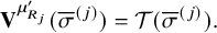 $$ \begin{align} \mathbf{V}^{\mu_{R_j}^{\prime}} (\overline{\sigma}^{(j)}) = \mathcal{T}(\overline{\sigma}^{(j)}). \end{align} $$
Assume that there exists an LDS $\overline {\eta }$
of
$\overline {\eta }$
of $\overline {\sigma }^{(j)}$
of length
$\overline {\sigma }^{(j)}$
of length $\ell ( \overline {\eta } ) = L> \mu _{R_j}^{\prime }$
. Then, by Proposition 6.8 there will exist an LDS
$\ell ( \overline {\eta } ) = L> \mu _{R_j}^{\prime }$
. Then, by Proposition 6.8 there will exist an LDS $\overline {\eta }^{(s)} \subset \mathbf {V}^{s}(\overline {\sigma }^{(j)})$
such that
$\overline {\eta }^{(s)} \subset \mathbf {V}^{s}(\overline {\sigma }^{(j)})$
such that $\ell ( \overline {\eta }^{(s)} ) = L$
, for all
$\ell ( \overline {\eta }^{(s)} ) = L$
, for all $s \ge 1$
. Additionally, elements of
$s \ge 1$
. Additionally, elements of $\overline {\eta }^{(1)}$
can be assumed to lie on the only down-right loop
$\overline {\eta }^{(1)}$
can be assumed to lie on the only down-right loop $\varsigma $
resulting from the shadow line construction of points of
$\varsigma $
resulting from the shadow line construction of points of $\overline {\eta }$
. In particular,
$\overline {\eta }$
. In particular, $\overline {\eta }^{(1)}$
lies weakly ‘below’
$\overline {\eta }^{(1)}$
lies weakly ‘below’ $\mathbf {V}(\overline {\eta })$
in the sense that if
$\mathbf {V}(\overline {\eta })$
in the sense that if
 $$ \begin{align} \overline{\eta}^{(1)} = (a_1^{\prime},b_1^{\prime}) \to \cdots \to (a_L^{\prime},b_L^{\prime}) \qquad \text{and} \qquad \mathbf{V}(\overline{\eta}) = (a_1,b_1) \to \cdots \to (a_L,b_L), \end{align} $$
then $b_1^{\prime }\le b_1, \dots , b_L^{\prime }\le b_L$
. Inductively, one can show that for any s,
$b_1^{\prime }\le b_1, \dots , b_L^{\prime }\le b_L$
. Inductively, one can show that for any s, $\overline {\eta }^{(s)}$
lies ‘below’
$\overline {\eta }^{(s)}$
lies ‘below’ $\mathbf {V}^{s}(\overline {\eta })$
in the same sense. We can now compare the evolution of
$\mathbf {V}^{s}(\overline {\eta })$
in the same sense. We can now compare the evolution of $\overline {\sigma }^{(j)}$
with that of
$\overline {\sigma }^{(j)}$
with that of $\overline {\eta }$
under iteration of the Viennot map. Since
$\overline {\eta }$
under iteration of the Viennot map. Since $\overline {\eta }$
is a localized decreasing subsequence, it is true that
$\overline {\eta }$
is a localized decreasing subsequence, it is true that
 $$ \begin{align} \mathbf{V}^L(\overline{\eta}) = \mathcal{T}(\overline{\eta}). \end{align} $$
Combining this last equality with equation (6.8), we have
 $$ \begin{align} \mathbf{V}^{N L \mu_{R_j^{\prime}}} (\overline{\sigma}^{(j)}) = \mathcal{T}^{N L} (\overline{\sigma}^{(j)}), \qquad \mathbf{V}^{N L \mu_{R_j^{\prime}}} (\overline{\eta}) = \mathcal{T}^{N \mu_{R_j^{\prime}}} (\overline{\eta}), \end{align} $$
which for N large enough implies that $\mathcal {T}^{N L} (\overline {\sigma }^{(j)})$
and
$\mathcal {T}^{N L} (\overline {\sigma }^{(j)})$
and $\mathcal {T}^{N \mu _{R_j^{\prime }}} (\overline {\eta })$
lie far apart from each other, since
$\mathcal {T}^{N \mu _{R_j^{\prime }}} (\overline {\eta })$
lie far apart from each other, since $L> \mu _{R_j}^{\prime }$
. This is a contradiction since elements of
$L> \mu _{R_j}^{\prime }$
. This is a contradiction since elements of $\overline {\eta }^{(NL \mu _{R_j^{\prime }})}$
should lie below
$\overline {\eta }^{(NL \mu _{R_j^{\prime }})}$
should lie below $\mathcal {T}^{N \mu _{R_j^{\prime }}} (\overline {\eta })$
. Therefore, there cannot exist any LDS of
$\mathcal {T}^{N \mu _{R_j^{\prime }}} (\overline {\eta })$
. Therefore, there cannot exist any LDS of $\overline {\sigma }^{(j)}$
strictly longer than
$\overline {\sigma }^{(j)}$
strictly longer than $\mu _{R_j}^{\prime }$
. This shows that
$\mu _{R_j}^{\prime }$
. This shows that $D_s(\overline {\sigma }^{(j)}) = s \times \mu _{R_j}^{\prime }$
and hence completes the proof of our proposition.
$D_s(\overline {\sigma }^{(j)}) = s \times \mu _{R_j}^{\prime }$
and hence completes the proof of our proposition.
In the following proposition, we prove that partitions $\mu , \widetilde {\mu }$
defined through Greene invariants
$\mu , \widetilde {\mu }$
defined through Greene invariants $D_k, I_k$
are in fact equal.
$D_k, I_k$
are in fact equal.
Proposition 6.10. Let $\mu , \widetilde {\mu }$
be as in equations (6.3), (6.4). Then, for all
$\mu , \widetilde {\mu }$
be as in equations (6.3), (6.4). Then, for all $\overline {\pi } \in \mathbb {A}_{n,n}$
, we have
$\overline {\pi } \in \mathbb {A}_{n,n}$
, we have $\mu (\overline {\pi }) = \widetilde {\mu }(\overline {\pi })$
.
$\mu (\overline {\pi }) = \widetilde {\mu }(\overline {\pi })$
.
For the sake of the proof of Proposition 6.10, we introduce now statistics of weighted biwords $\overline {\pi }$
which are ‘dual’ to the Greene invariants
$\overline {\pi }$
which are ‘dual’ to the Greene invariants $D_k$
. Let
$D_k$
. Let $\mathfrak {D}(\overline {\pi })$
denote the set of decompositions of
$\mathfrak {D}(\overline {\pi })$
denote the set of decompositions of $\overline {\pi }$
into localised decreasing subsequences
$\overline {\pi }$
into localised decreasing subsequences
Given $\mathfrak {d} = (\overline {\sigma }^{(1)} ,\overline {\sigma }^{(2)}, \dots ) \in \mathfrak {D}(\overline {\pi })$
, define
$\mathfrak {d} = (\overline {\sigma }^{(1)} ,\overline {\sigma }^{(2)}, \dots ) \in \mathfrak {D}(\overline {\pi })$
, define
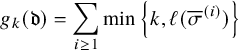 $$ \begin{align} g_k (\mathfrak{d}) = \sum_{i\ge 1} \min \left\{ k , \ell ( \overline{\sigma}^{(i)} ) \right\} \end{align} $$
and
 $$ \begin{align} G_k(\overline{\pi}) = \min_{\mathfrak{d} \in \mathfrak{D}(\overline{\pi}) } g_k (\mathfrak{d}). \end{align} $$
In words, $g_k$
tells us how ‘spread out’ the decomposition
$g_k$
tells us how ‘spread out’ the decomposition $\mathfrak {d}$
is, as in the summation localized decreasing subsequences longer than k contribute with a penalized weight. On the other hand, statistics
$\mathfrak {d}$
is, as in the summation localized decreasing subsequences longer than k contribute with a penalized weight. On the other hand, statistics $G_k$
record how likely it is to decompose
$G_k$
record how likely it is to decompose $\overline {\pi }$
in the least number of localized decreasing subsequences. We have the following.
$\overline {\pi }$
in the least number of localized decreasing subsequences. We have the following.
Lemma 6.11. Let $\overline {\pi } \in \overline {\mathbb {A}}_{n,n}$
, take
$\overline {\pi } \in \overline {\mathbb {A}}_{n,n}$
, take $\mu $
as in equation (6.3), and define
$\mu $
as in equation (6.3), and define $\varkappa $
as
$\varkappa $
as
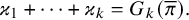 $$ \begin{align} \varkappa_1 + \cdots + \varkappa_k = G_k(\overline{\pi}). \end{align} $$
Then $\mu = \varkappa $
.
$\mu = \varkappa $
.
Proof. Let
![]() be a maximising k-LDS of
be a maximising k-LDS of $\overline {\pi }$
, or in other words assume that
$\overline {\pi }$
, or in other words assume that $\ell ( \overline {\sigma }^{(1)} ) + \cdots + \ell ( \overline {\sigma }^{(k)} ) = \mu _1^{\prime } + \cdots + \mu _k^{\prime }$
. It is clear that
$\ell ( \overline {\sigma }^{(1)} ) + \cdots + \ell ( \overline {\sigma }^{(k)} ) = \mu _1^{\prime } + \cdots + \mu _k^{\prime }$
. It is clear that $\ell ( \overline {\sigma }^{(j)} ) \ge \mu _k^{\prime }$
for all j. Otherwise, say
$\ell ( \overline {\sigma }^{(j)} ) \ge \mu _k^{\prime }$
for all j. Otherwise, say $\ell ( \overline {\sigma }^{(k)} ) \le \mu _k^{\prime }-1$
, then this would imply that
$\ell ( \overline {\sigma }^{(k)} ) \le \mu _k^{\prime }-1$
, then this would imply that $\ell ( \overline {\sigma }^{(1)} ) + \cdots + \ell ( \overline {\sigma }^{(k-1)} ) \ge \mu _1^{\prime } + \cdots + \mu _{k-1}^{\prime } +1$
, which contradicts the definition of
$\ell ( \overline {\sigma }^{(1)} ) + \cdots + \ell ( \overline {\sigma }^{(k-1)} ) \ge \mu _1^{\prime } + \cdots + \mu _{k-1}^{\prime } +1$
, which contradicts the definition of $\mu $
. Let
$\mu $
. Let $\mathfrak {d} = (\overline {\sigma }^{(1)},\dots ,\overline {\sigma }^{(k)},\overline {\eta }^{(k+1)},\dots ) \in \mathfrak {D}(\overline {\pi })$
, where
$\mathfrak {d} = (\overline {\sigma }^{(1)},\dots ,\overline {\sigma }^{(k)},\overline {\eta }^{(k+1)},\dots ) \in \mathfrak {D}(\overline {\pi })$
, where $\overline {\eta }^{(l)}, l>k$
are LDSs formed with elements of
$\overline {\eta }^{(l)}, l>k$
are LDSs formed with elements of $\overline {\pi } \setminus \overline {\sigma }$
and notice that
$\overline {\pi } \setminus \overline {\sigma }$
and notice that $\ell ( \mathfrak {d} ) = |\mu |$
. Similarly as above, each
$\ell ( \mathfrak {d} ) = |\mu |$
. Similarly as above, each $\overline {\eta }^{(l)}$
has length which is no longer than
$\overline {\eta }^{(l)}$
has length which is no longer than $\mu _k^{\prime }$
. Then
$\mu _k^{\prime }$
. Then
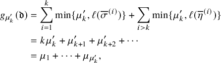 $$ \begin{align} \begin{aligned} g_{\mu_k^{\prime}}(\mathfrak{d}) &= \sum_{i=1}^{k} \min\{ \mu_k^{\prime} , \ell ( \overline{\sigma}^{(i)} ) \} + \sum_{i>k} \min\{ \mu_k^{\prime} , \ell ( \overline{\eta}^{(i)} ) \} \\ &= k \mu_k^{\prime} + \mu_{k+1}^{\prime} + \mu_{k+2}^{\prime} + \cdots \\ & = \mu_1 + \cdots + \mu_{\mu_k^{\prime}}, \end{aligned} \end{align} $$
which implies $\varkappa _1 + \cdots +\varkappa _{\mu _k^{\prime }} \le \mu _1 + \cdots +\mu _{\mu _k^{\prime }}$
. Assume that this last inequality can be made strict. This means that we can find
$\varkappa _1 + \cdots +\varkappa _{\mu _k^{\prime }} \le \mu _1 + \cdots +\mu _{\mu _k^{\prime }}$
. Assume that this last inequality can be made strict. This means that we can find $\mathfrak {d}' = (\overline {\xi }^{(1)},\overline {\xi }^{(2)},\dots )$
, with LDSs arranged decreasingly in length, such that
$\mathfrak {d}' = (\overline {\xi }^{(1)},\overline {\xi }^{(2)},\dots )$
, with LDSs arranged decreasingly in length, such that
 $$ \begin{align} g_{\mu_k^{\prime}}(\mathfrak{d}') = m \mu_k^{\prime} + \ell ( \overline{\xi}^{(m + 1)} ) + \ell ( \overline{\xi}^{(m +2)} ) +\cdots < k \mu_k^{\prime} + \mu_{k+1}^{\prime} + \mu_{k+2}^{\prime} + \cdots, \end{align} $$
where m is the number of LDSs $\overline {\xi }^{(j)}$
with length greater than or equal to
$\overline {\xi }^{(j)}$
with length greater than or equal to $\mu _{k}^{\prime }$
. Since
$\mu _{k}^{\prime }$
. Since $\ell ( \overline {\xi }^{(1)} ) + \cdots + \ell ( \overline {\xi }^{(m)} ) \le \mu _1^{\prime } + \cdots +\mu _m^{\prime } $
we have
$\ell ( \overline {\xi }^{(1)} ) + \cdots + \ell ( \overline {\xi }^{(m)} ) \le \mu _1^{\prime } + \cdots +\mu _m^{\prime } $
we have
 $$ \begin{align} \mu_{m +1}^{\prime} + \mu_{m+2}^{\prime} +\cdots \le \ell ( \overline{\xi}^{(m +1)} ) + \ell ( \overline{\xi}^{(m +2)} ) +\cdots, \end{align} $$
which implies the inequality
 $$ \begin{align} (\mu_{m +1 }^{\prime} + \mu_{m+2}^{\prime} +\cdots ) - (\mu_{k +1 }^{\prime} + \mu_{k+2}^{\prime} +\cdots ) < (k -m) \mu_k^{\prime}. \end{align} $$
In case $m<k$
, equation (6.19) becomes
$m<k$
, equation (6.19) becomes $\mu _{m + 1 }^{\prime } + \cdots + \mu _{k}^{\prime } < (k - m) \mu _k^{\prime }$
, which is impossible since terms of
$\mu _{m + 1 }^{\prime } + \cdots + \mu _{k}^{\prime } < (k - m) \mu _k^{\prime }$
, which is impossible since terms of $\mu $
are weakly decreasing. Alternatively, in case
$\mu $
are weakly decreasing. Alternatively, in case $m \ge k$
, equation (6.19) becomes
$m \ge k$
, equation (6.19) becomes $(m - k) \mu _k^{\prime } < \mu _{k+1}^{\prime } +\cdots + \mu _m^{\prime }$
, which is also impossible for the same reason. Therefore,
$(m - k) \mu _k^{\prime } < \mu _{k+1}^{\prime } +\cdots + \mu _m^{\prime }$
, which is also impossible for the same reason. Therefore, $\varkappa _1 + \cdots + \varkappa _{\mu _k^{\prime }} = \mu _1 + \cdots + \mu _{\mu _k^{\prime }}$
for all k and this completes the proof.
$\varkappa _1 + \cdots + \varkappa _{\mu _k^{\prime }} = \mu _1 + \cdots + \mu _{\mu _k^{\prime }}$
for all k and this completes the proof.
Lemma 6.12. Let $\overline {\pi } \in \overline {\mathbb {A}}_{n,n}$
, and consider partitions
$\overline {\pi } \in \overline {\mathbb {A}}_{n,n}$
, and consider partitions $\mu , \widetilde {\mu }$
as in equations (6.3), (6.4). Then
$\mu , \widetilde {\mu }$
as in equations (6.3), (6.4). Then $\widetilde {\mu } \trianglelefteq \mu $
, where “
$\widetilde {\mu } \trianglelefteq \mu $
, where “ $\trianglelefteq $
” is the dominance order
$\trianglelefteq $
” is the dominance order $\widetilde {\mu }_1+\cdots + \widetilde {\mu }_k \le \mu _1+\cdots + \mu _k$
for all k.
$\widetilde {\mu }_1+\cdots + \widetilde {\mu }_k \le \mu _1+\cdots + \mu _k$
for all k.
Proof. Let $\mathfrak {d}=(\overline {\sigma }^{(1)},\overline {\sigma }^{(2)}, \dots ) \in \mathfrak {D}(\overline {\pi })$
, and consider k disjoint increasing subsequences
$\mathfrak {d}=(\overline {\sigma }^{(1)},\overline {\sigma }^{(2)}, \dots ) \in \mathfrak {D}(\overline {\pi })$
, and consider k disjoint increasing subsequences $\overline {\eta }^{(1)} ,\dots , \overline {\eta }^{(k)}$
of
$\overline {\eta }^{(1)} ,\dots , \overline {\eta }^{(k)}$
of $\overline {\pi }$
. For any i and j, the intersection
$\overline {\pi }$
. For any i and j, the intersection $\overline {\eta }^{(i)} \cap \overline {\sigma }^{(j)}$
has at most one element; therefore, we have
$\overline {\eta }^{(i)} \cap \overline {\sigma }^{(j)}$
has at most one element; therefore, we have
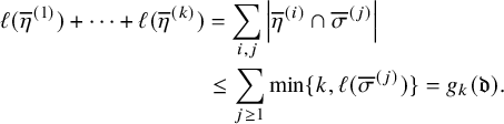 $$ \begin{align} \begin{aligned}\ell ( \overline{\eta}^{(1)} ) + \cdots + \ell ( \overline{\eta}^{(k)} ) & = \sum_{i,j} \left| \overline{\eta}^{(i)} \cap \overline{\sigma}^{(j)} \right| \\&\le \sum_{j \ge 1} \min\{ k, \ell ( \overline{\sigma}^{(j)} ) \} = g_k(\mathfrak{d}). \end{aligned} \end{align} $$
Minimizing the right-hand side over $\mathfrak {d}$
we obtain that
$\mathfrak {d}$
we obtain that $\ell ( \overline {\eta }^{(1)} ) + \cdots + \ell ( \overline {\eta }^{(k)} ) \le G_k (\overline {\pi })$
and hence
$\ell ( \overline {\eta }^{(1)} ) + \cdots + \ell ( \overline {\eta }^{(k)} ) \le G_k (\overline {\pi })$
and hence $I_k(\overline {\pi }) \le G_k (\overline {\pi })$
maximizing over the choice of increasing subsequences
$I_k(\overline {\pi }) \le G_k (\overline {\pi })$
maximizing over the choice of increasing subsequences $\overline {\eta }^{(i)}$
. We can now use Proposition 6.11 to identify
$\overline {\eta }^{(i)}$
. We can now use Proposition 6.11 to identify $G_k(\overline {\pi })$
with
$G_k(\overline {\pi })$
with $\mu _1 + \cdots + \mu _k$
, completing the proof.
$\mu _1 + \cdots + \mu _k$
, completing the proof.
Lemma 6.13. Consider $\overline {\pi } \in \overline {\mathbb {A}}_{n,n}$
as in equation (2.1), its p-word
$\overline {\pi } \in \overline {\mathbb {A}}_{n,n}$
as in equation (2.1), its p-word $p(\overline {\pi })=p_1\cdots p_{\ell (\overline {\pi })}$
and its content
$p(\overline {\pi })=p_1\cdots p_{\ell (\overline {\pi })}$
and its content $\gamma =\gamma (p(\overline {\pi }))$
. Then, in the dominance order,
$\gamma =\gamma (p(\overline {\pi }))$
. Then, in the dominance order, $\gamma ^+ \trianglelefteq \widetilde {\mu }$
, where
$\gamma ^+ \trianglelefteq \widetilde {\mu }$
, where $\widetilde {\mu }$
is given by (6.4).
$\widetilde {\mu }$
is given by (6.4).
Proof. Consider the subwords $\overline {\sigma }^{(i)} \subseteq \overline {\pi }$
formed by all elements of
$\overline {\sigma }^{(i)} \subseteq \overline {\pi }$
formed by all elements of $\overline {\pi }$
of the form
$\overline {\pi }$
of the form $\left ( \begin {smallmatrix} q_j \\ i \\ w_j \end {smallmatrix} \right )$
. Then
$\left ( \begin {smallmatrix} q_j \\ i \\ w_j \end {smallmatrix} \right )$
. Then $\overline {\sigma }^{(i)}$
are increasing subsequences as each cell
$\overline {\sigma }^{(i)}$
are increasing subsequences as each cell $[\overline {\sigma }^{(i)}_j]$
is contained in the up-right path
$[\overline {\sigma }^{(i)}_j]$
is contained in the up-right path $\varpi ^{(i)}=\mathbb {Z} \times \{i\}$
. Since
$\varpi ^{(i)}=\mathbb {Z} \times \{i\}$
. Since $\ell ( \overline {\sigma }^{(i)} ) = \gamma _i$
we have, for all k
$\ell ( \overline {\sigma }^{(i)} ) = \gamma _i$
we have, for all k
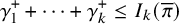 $$ \begin{align} \gamma_1^+ + \cdots + \gamma_k^+ \le I_k(\overline{\pi}) \end{align} $$
and hence $\gamma ^+ \trianglelefteq \widetilde {\mu }$
.
$\gamma ^+ \trianglelefteq \widetilde {\mu }$
.
Lemma 6.14. Consider $\overline {\pi } \in \overline {\mathbb {A}}_{n,n}$
, and let
$\overline {\pi } \in \overline {\mathbb {A}}_{n,n}$
, and let $\mu =\mu (\overline {\pi })$
be as in (6.3). Then there exists a transformation h, which is composition of Kashiwara operators
$\mu =\mu (\overline {\pi })$
be as in (6.3). Then there exists a transformation h, which is composition of Kashiwara operators $\widetilde {E}^{(1)}_i,\widetilde {F}^{(1)}_i$
for
$\widetilde {E}^{(1)}_i,\widetilde {F}^{(1)}_i$
for $i=0,\dots ,n-1$
such that, denoting
$i=0,\dots ,n-1$
such that, denoting $\overline {\pi }'= h(\overline {\pi })$
, we have
$\overline {\pi }'= h(\overline {\pi })$
, we have $\gamma (p(\overline {\pi }')) = \mu $
.
$\gamma (p(\overline {\pi }')) = \mu $
.
Proof. Let $(P,Q)$
be a pair of tableaux such that
$(P,Q)$
be a pair of tableaux such that $(P,Q) \xrightarrow []{\mathbf {SS} \,} \overline {\pi }$
and denote by
$(P,Q) \xrightarrow []{\mathbf {SS} \,} \overline {\pi }$
and denote by $\mu $
the asymptotic increment. By Proposition 6.9, we have
$\mu $
the asymptotic increment. By Proposition 6.9, we have $\mu =\mu (\overline {\pi })$
. The projection
$\mu =\mu (\overline {\pi })$
. The projection $\Phi $
acts on such pair as
$\Phi $
acts on such pair as $\Phi (P,Q) = (V,W)$
with
$\Phi (P,Q) = (V,W)$
with $V,W \in VST(\mu ,n)$
. Viewed as an affine crystal graph,
$V,W \in VST(\mu ,n)$
. Viewed as an affine crystal graph, $VTS(\mu ,n)$
is connected, by Proposition 5.4 and hence there exists a map
$VTS(\mu ,n)$
is connected, by Proposition 5.4 and hence there exists a map $h_V = \widetilde {e}_{i_1}^{N_1} \circ \widetilde {f}_{i_2}^{N_2} \circ \cdots $
such that
$h_V = \widetilde {e}_{i_1}^{N_1} \circ \widetilde {f}_{i_2}^{N_2} \circ \cdots $
such that $h_V(V) = \mu ^{\mathrm {lv}}$
, where as in Section 5.3,
$h_V(V) = \mu ^{\mathrm {lv}}$
, where as in Section 5.3, $\mu ^{\mathrm {lv}}$
denotes the unique vertically strict tableau of shape
$\mu ^{\mathrm {lv}}$
denotes the unique vertically strict tableau of shape $\mu $
and content
$\mu $
and content $\mu $
. We can lift the action of the map
$\mu $
. We can lift the action of the map $h_V$
to the set of pairs
$h_V$
to the set of pairs $(V',W')$
defining
$(V',W')$
defining $h=h_V \times \mathbf {1} : (V',W') \mapsto (h_V(V'),W')$
. Further, as in Section 5.4 we consider the
$h=h_V \times \mathbf {1} : (V',W') \mapsto (h_V(V'),W')$
. Further, as in Section 5.4 we consider the $\Phi $
-pullback map of h that acts on pairs of skew tableaux as
$\Phi $
-pullback map of h that acts on pairs of skew tableaux as $h=\left (\widetilde {E}^{(1)}_{i_1}\right )^{N_1} \circ \left (\widetilde {F}^{(1)}_{i_2}\right )^{N_2} \circ \cdots $
. Then, by Proposition 5.9, we have
$h=\left (\widetilde {E}^{(1)}_{i_1}\right )^{N_1} \circ \left (\widetilde {F}^{(1)}_{i_2}\right )^{N_2} \circ \cdots $
. Then, by Proposition 5.9, we have $h(P,Q)=(P',Q')$
with
$h(P,Q)=(P',Q')$
with $\gamma (P') = \mu $
. By the fact that projection
$\gamma (P') = \mu $
. By the fact that projection $(P,Q)\xrightarrow []{\mathbf {SS}\,} \overline {\pi }$
is a morphism of bicrystals, we define
$(P,Q)\xrightarrow []{\mathbf {SS}\,} \overline {\pi }$
is a morphism of bicrystals, we define $(P',Q') \xrightarrow []{\mathbf {SS}\,} \overline {\pi }'$
and
$(P',Q') \xrightarrow []{\mathbf {SS}\,} \overline {\pi }'$
and $\gamma (p(\overline {\pi }')) = \mu $
.
$\gamma (p(\overline {\pi }')) = \mu $
.
This leads up to the proof of Proposition 6.10.
Proof of Proposition 6.10.
By Proposition 6.12, we have $\widetilde {\mu }(\overline {\pi }) \trianglelefteq \mu (\overline {\pi })$
. Moreover, by Proposition 6.14, we can always find a composition of Kashiwara operators h such that
$\widetilde {\mu }(\overline {\pi }) \trianglelefteq \mu (\overline {\pi })$
. Moreover, by Proposition 6.14, we can always find a composition of Kashiwara operators h such that $h(\overline {\pi })=\overline {\pi }'$
and
$h(\overline {\pi })=\overline {\pi }'$
and $\gamma (p(\overline {\pi }')) = \mu (\overline {\pi })$
. By Proposition 6.4, we have
$\gamma (p(\overline {\pi }')) = \mu (\overline {\pi })$
. By Proposition 6.4, we have $\mu (\overline {\pi }') = \mu (\overline {\pi })$
so that by Proposition 6.13 we can conclude that also
$\mu (\overline {\pi }') = \mu (\overline {\pi })$
so that by Proposition 6.13 we can conclude that also $\mu (\overline {\pi }) \trianglelefteq \widetilde {\mu } (\overline {\pi })$
. Therefore,
$\mu (\overline {\pi }) \trianglelefteq \widetilde {\mu } (\overline {\pi })$
. Therefore, $\mu (\overline {\pi }) = \widetilde {\mu } (\overline {\pi })$
.
$\mu (\overline {\pi }) = \widetilde {\mu } (\overline {\pi })$
.
We can finally prove our main results of the section.
Proof of Proposition 6.5.
The fact that the Viennot map preserves statistics $D_k$
is the result of Proposition 6.8. This also implies that the partition
$D_k$
is the result of Proposition 6.8. This also implies that the partition $\mu (\overline {\pi })$
defined as in equation (6.3) is invariant. The fact that also
$\mu (\overline {\pi })$
defined as in equation (6.3) is invariant. The fact that also $I_k$
’s are invariant under
$I_k$
’s are invariant under $\mathbf {V}$
follows from Proposition 6.10, which implies the chain of equalities
$\mathbf {V}$
follows from Proposition 6.10, which implies the chain of equalities
 $$ \begin{align} \widetilde{\mu}(\mathbf{V}(\overline{\pi})) = \mu(\mathbf{V}(\overline{\pi})) = \mu (\overline{\pi}) = \widetilde{\mu}(\overline{\pi}). \end{align} $$
This concludes the proof.
Proof of Proposition 6.6.
By Proposition 6.9, the asymptotic increment $\mu (P,Q)$
is always equal to the partition
$\mu (P,Q)$
is always equal to the partition $\mu (\overline {\pi })$
, whenever
$\mu (\overline {\pi })$
, whenever $(P,Q) \xrightarrow []{\mathbf {SS}\,} \overline {\pi }$
. Proposition 6.10 then provides the equalities
$(P,Q) \xrightarrow []{\mathbf {SS}\,} \overline {\pi }$
. Proposition 6.10 then provides the equalities $\mu (P,Q) = \mu (\overline {\pi }) = \widetilde {\mu }(\overline {\pi })$
.
$\mu (P,Q) = \mu (\overline {\pi }) = \widetilde {\mu }(\overline {\pi })$
.
7 Energy function, Demazure crystals and linearization of dynamics
7.1 Combinatorial
$\mathscr {R}$
matrix and energy function

For any $r_1,r_2 \in \mathbb {N}$
, crystal graphs
$r_1,r_2 \in \mathbb {N}$
, crystal graphs $\widehat {B}(r_1,r_2)$
and
$\widehat {B}(r_1,r_2)$
and $\widehat {B}(r_2,r_1)$
are isomorphic, via a unique isomorphism of crystal graphs called combinatorial
$\widehat {B}(r_2,r_1)$
are isomorphic, via a unique isomorphism of crystal graphs called combinatorial $\mathscr {R}$
matrix
$\mathscr {R}$
matrix
 $$ \begin{align}\mathscr{R}:B^{r_1,1} \otimes B^{r_2,1} \to B^{r_2,1} \otimes B^{r_1,1}. \end{align} $$
There exists a number of equivalent definitions of $\mathscr {R}$
(see [Reference Kang, Kashiwara, Misra, Miwa, Nakashima and Nakayashiki48, Reference Nakayashiki and Yamada65, Reference Shimozono80]), and the one reported below is a reformulation of the original algorithm by Nakayashiki and Yamada as in Rule 3.10 of [Reference Nakayashiki and Yamada65]. Consider
$\mathscr {R}$
(see [Reference Kang, Kashiwara, Misra, Miwa, Nakashima and Nakayashiki48, Reference Nakayashiki and Yamada65, Reference Shimozono80]), and the one reported below is a reformulation of the original algorithm by Nakayashiki and Yamada as in Rule 3.10 of [Reference Nakayashiki and Yamada65]. Consider $b_i \in B^{r_i,1}$
for
$b_i \in B^{r_i,1}$
for $i=1,2$
and we want to find
$i=1,2$
and we want to find $\tilde {b}_i \in B^{r_i,1}$
such that
$\tilde {b}_i \in B^{r_i,1}$
such that
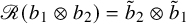 $$ \begin{align} \mathscr{R}(b_1 \otimes b_2) = \tilde{b}_2 \otimes \tilde{b}_1 \end{align} $$
by shifting cells from one column to the other. The procedure goes as follows.
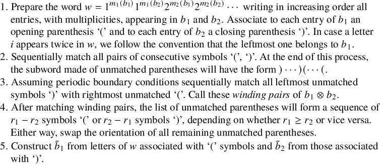 $$ \begin{align}&1. \ \text{Prepare the word } w = 1^{m_1(b_1)} 1^{m_1(b_2)} 2^{m_2(b_1)} 2^{m_2(b_2)} \cdots \text{ writing in increasing order all}\nonumber\\[-3pt]&\quad \text{entries, with multiplicities, appearing in } b_1 \text{ and } b_2. \text{ Associate to each entry of } b_1 \text{ an }\nonumber\\[-3pt]&\quad \text{opening parenthesis `(' and to each entry of } b_2 \text{ a closing parenthesis `)'. In case a letter }\nonumber\\[-3pt]&\quad i \text{ appears twice in } w\text{, we follow the convention that the leftmost one belongs to } b_1.\nonumber\\[-3pt]&2. \ \text{Sequentially match all pairs of consecutive symbols `(', `)'. At the end of this process,}\nonumber\\[-3pt]&\quad \text{the subword made of unmatched parentheses will have the form } )\cdots ) ( \cdots (.\nonumber\\[-3pt]&3. \ \text{Assuming periodic boundary conditions sequentially match all leftmost unmatched} \\[-3pt]&\quad \text{symbols `)' with rightmost unmatched `('. Call these } \textit{winding pairs} \text{ of } b_1 \otimes b_2.\nonumber\\[-3pt]&4. \ \text{After matching winding pairs, the list of unmatched parentheses will form a sequence of }\nonumber\\[-3pt]&\quad r_1 - r_2 \text{ symbols `(' or } r_2 - r_1 \text{ symbols `)', depending on whether } r_1 \ge r_2 \text{ or vice versa. }\nonumber\\[-3pt]&\quad \text{Either way, swap the orientation of all remaining unmatched parentheses.}\nonumber\\[-3pt]&5. \ \text{Construct } \tilde{b}_1 \text{ from letters of } w \text{ associated with `(' symbols and } \tilde{b}_2 \text{ from those associated}\nonumber\\[-3pt]&\quad \text{with `)'.}\nonumber \end{align} $$
We also define the energy function
 $$ \begin{align} H(b_1 \otimes b_2) = \text{number of winding pairs of }b_1 \otimes b_2. \end{align} $$
To have a better understanding of the algorithm for $\mathscr {R}$
consider the following example.
$\mathscr {R}$
consider the following example.
Example 7.1. In the evaluation below, we have $r_1=3$
and
$r_1=3$
and $r_2=4$
:
$r_2=4$
:
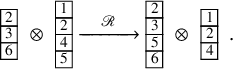
This follows from the construction
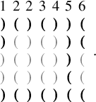
Notice that in the fourth line we matched the only winding pair of parenthesis as for (3) of equation (7.3). This in particular implies that in this case we have $H(b_1\otimes b_2)=1$
.
$H(b_1\otimes b_2)=1$
.
Remark 7.2. The combinatorial $\mathscr {R}$
matrix, as the name suggests, satisfies the Yang–Baxter equation
$\mathscr {R}$
matrix, as the name suggests, satisfies the Yang–Baxter equation
 $$ \begin{align} (\mathscr{R} \otimes \mathbf{1}) (\mathbf{1} \otimes \mathscr{R}) (\mathscr{R} \otimes \mathbf{1}) = (\mathbf{1} \otimes \mathscr{R}) (\mathscr{R} \otimes \mathbf{1}) (\mathbf{1} \otimes \mathscr{R}) \end{align} $$
and can be also defined as the $q \to 0$
limit of the fused
$q \to 0$
limit of the fused $\mathscr {R}$
matrix of
$\mathscr {R}$
matrix of $\mathcal {U}_q(\widehat {sl}_{n})$
. We will not make use of this fact in this paper, but the interested reader can consult [Reference Kang, Kashiwara, Misra, Miwa, Nakashima and Nakayashiki48, Reference Shimozono80].
$\mathcal {U}_q(\widehat {sl}_{n})$
. We will not make use of this fact in this paper, but the interested reader can consult [Reference Kang, Kashiwara, Misra, Miwa, Nakashima and Nakayashiki48, Reference Shimozono80].
We use the notation $\mathscr {R}_i$
to denote the
$\mathscr {R}_i$
to denote the $\mathscr {R}$
-matrix acting only on the i-th and
$\mathscr {R}$
-matrix acting only on the i-th and $(i+1)$
-th component of a tensor product
$(i+1)$
-th component of a tensor product $b_1\otimes \cdots \otimes b_N$
 $$ \begin{align} \mathscr{R}_i = \mathbf{1}^{\otimes (i-1)} \otimes \mathscr{R} \otimes \mathbf{1}^{\otimes (N-i)}. \end{align} $$
Proposition 7.3. Consider a permutation $\sigma = \sigma _{i_1} \cdots \sigma _{i_M}$
written as a product of elementary transpositions
$\sigma = \sigma _{i_1} \cdots \sigma _{i_M}$
written as a product of elementary transpositions $\sigma _i$
that exchange i and
$\sigma _i$
that exchange i and $i+1$
. Fix compositions
$i+1$
. Fix compositions $\varkappa =(\varkappa _1,\dots ,\varkappa _N)$
,
$\varkappa =(\varkappa _1,\dots ,\varkappa _N)$
, $\eta =(\varkappa _{\sigma (1)},\dots ,\varkappa _{\sigma (N)})$
. Then,
$\eta =(\varkappa _{\sigma (1)},\dots ,\varkappa _{\sigma (N)})$
. Then,
 $$ \begin{align} \mathscr{R}_{\sigma} = \mathscr{R}_{i_1} \cdots \mathscr{R}_{i_M} : B^\varkappa \to B^\eta \end{align} $$
is the unique isomorphism of crystal graphs $B^\varkappa \to B^\eta $
.
$B^\varkappa \to B^\eta $
.
Proof. Composition of isomorphisms of crystal graphs is still an isomorphism of crystal graphs. This shows that $\mathscr {R}_{\sigma }:B^\varkappa \to B^\eta $
is an isomorphism of crystal graphs and it is the only one, by Proposition 5.5.
$\mathscr {R}_{\sigma }:B^\varkappa \to B^\eta $
is an isomorphism of crystal graphs and it is the only one, by Proposition 5.5.
A theorem in [Reference Kang, Kashiwara, Misra, Miwa, Nakashima and Nakayashiki48] describes how the energy function changes under the action of the crystal operators. Assuming that $\mathscr {R}(b_1 \otimes b_2)= \tilde {b}_2 \otimes \tilde {b}_1$
, we have
$\mathscr {R}(b_1 \otimes b_2)= \tilde {b}_2 \otimes \tilde {b}_1$
, we have
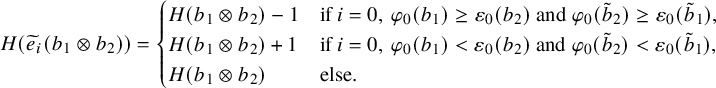 $$ \begin{align} H(\widetilde{e}_{i}(b_1 \otimes b_2)) = \begin{cases} H(b_1 \otimes b_2) - 1 \qquad & \text{if } i=0, \,\varphi_0(b_1) \ge \varepsilon_0(b_2) \text{ and } \varphi_0(\tilde{b}_2) \ge \varepsilon_0(\tilde{b}_1), \\ H(b_1 \otimes b_2) + 1 \qquad & \text{if } i=0, \,\varphi_0(b_1) < \varepsilon_0(b_2) \text{ and } \varphi_0(\tilde{b}_2) < \varepsilon_0(\tilde{b}_1), \\ H(b_1 \otimes b_2) & \text{else}. \end{cases} \end{align} $$
Just as we associate an energy function to a tensor product of two elements $b_1 \otimes b_2$
, there exists a canonical way of defining an energy on arbitrary finite products
$b_1 \otimes b_2$
, there exists a canonical way of defining an energy on arbitrary finite products $b_1 \otimes \cdots \otimes b_N$
.
$b_1 \otimes \cdots \otimes b_N$
.
Definition 7.4 (Intrinsic energy).
Consider a composition $\varkappa =(\varkappa _1,\dots , \varkappa _N)$
. For any
$\varkappa =(\varkappa _1,\dots , \varkappa _N)$
. For any $b=b_1 \otimes \cdots \otimes b_N \in B^\varkappa $
, the local energies
$b=b_1 \otimes \cdots \otimes b_N \in B^\varkappa $
, the local energies $\mathscr {H}_i$
and the intrinsic energy
$\mathscr {H}_i$
and the intrinsic energy $\mathscr {H}$
are the functions
$\mathscr {H}$
are the functions
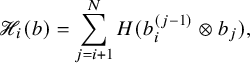 $$ \begin{align} \mathscr{H}_i (b) = \sum_{j=i+1}^N H (b_i^{(j-1)} \otimes b_j), \end{align} $$
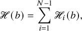 $$ \begin{align} \mathscr{H}(b) = \sum_{i=1}^{N-1} \mathscr{H}_i (b), \end{align} $$
where $b^{(i)}_i=b_i$
and
$b^{(i)}_i=b_i$
and $b_i^{(j-1)}$
is defined recursively by
$b_i^{(j-1)}$
is defined recursively by
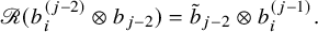 $$ \begin{align} \mathscr{R}(b_i^{(j-2)} \otimes b_{j-2}) = \tilde{b}_{j-2} \otimes b_i^{(j-1)}. \end{align} $$
The intrinsic energy $\mathscr {H}$
is, as all the local energies
$\mathscr {H}$
is, as all the local energies $\mathscr {H}_i$
are, constant on classical connected components of
$\mathscr {H}_i$
are, constant on classical connected components of $\widehat {B}(\varkappa )$
. This is a consequence of equation (7.10) and of the fact that the combinatorial
$\widehat {B}(\varkappa )$
. This is a consequence of equation (7.10) and of the fact that the combinatorial $\mathscr {R}$
matrix commutes with Kashiwara operators.
$\mathscr {R}$
matrix commutes with Kashiwara operators.
7.2 Demazure subgraph
For an affine crystal graph $\widehat {B}(\varkappa )$
, we define its Demazure subgraph
$\widehat {B}(\varkappa )$
, we define its Demazure subgraph $\widetilde {B}(\varkappa )$
. Its set of vertices is
$\widetilde {B}(\varkappa )$
. Its set of vertices is $B^\varkappa $
, while its edges, called Demazure arrows, are defined next.
$B^\varkappa $
, while its edges, called Demazure arrows, are defined next.
The affine crystal graph $\widehat {B}(\varkappa )$
, for
$\widehat {B}(\varkappa )$
, for $\varkappa =(2,1,1)$
. Edges
$\varkappa =(2,1,1)$
. Edges $\xrightarrow []{i}$
are defined by the action of
$\xrightarrow []{i}$
are defined by the action of $\widetilde {f}_{i}$
. Black arrows define the classical crystal graph
$\widetilde {f}_{i}$
. Black arrows define the classical crystal graph $B(\varkappa )$
. Blue arrows denote 0-Demazure arrows so that the Demazure subgraph
$B(\varkappa )$
. Blue arrows denote 0-Demazure arrows so that the Demazure subgraph $\widetilde {B}(\varkappa )$
consists in black and blue edges. Red arrows are 0-arrows that are not Demazure arrows. Notice the defining property of 0-Demazure arrows, that always originate from vertices b that are endpoints of
$\widetilde {B}(\varkappa )$
consists in black and blue edges. Red arrows are 0-arrows that are not Demazure arrows. Notice the defining property of 0-Demazure arrows, that always originate from vertices b that are endpoints of $0$
-arrows.
$0$
-arrows.
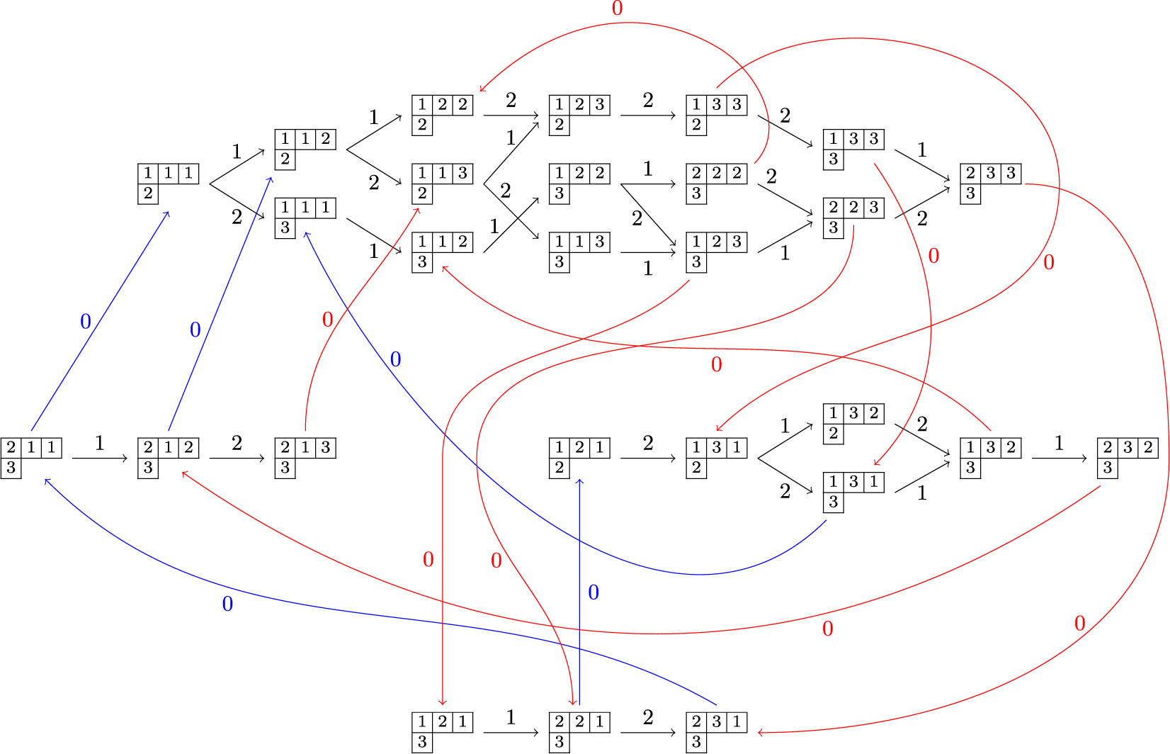
Definition 7.5 (Demazure arrows).
Let $b \in B^{\varkappa }$
. We say that
$b \in B^{\varkappa }$
. We say that $b \rightarrow \widetilde {f}_{i}(b)$
is a Demazure arrow if
$b \rightarrow \widetilde {f}_{i}(b)$
is a Demazure arrow if $i=1,\dots , n-1$
, or if
$i=1,\dots , n-1$
, or if $i=0$
and
$i=0$
and $\varepsilon _0(b)> 0$
. Equivalently,
$\varepsilon _0(b)> 0$
. Equivalently, $b\rightarrow \widetilde {e}_{i}(b)$
is a Demazure arrow if
$b\rightarrow \widetilde {e}_{i}(b)$
is a Demazure arrow if $i=1,\dots ,n-1$
, or if
$i=1,\dots ,n-1$
, or if $i=0$
and
$i=0$
and $\varepsilon _0(b)>1$
.
$\varepsilon _0(b)>1$
.
An example of a Demazure subgraph is shown in Figure 18. Notice that the Demazure subgraph is not a crystal graph as in the definition given in Section 5.1. In fact, $\widetilde {B}(\varkappa )$
is the image under a canonical isomorphsm, denoted by j in [Reference Schilling and Tingley77], of the corresponding Demazure crystal [Reference Bump and Schilling16, Chapter 13]. For this reason,
$\widetilde {B}(\varkappa )$
is the image under a canonical isomorphsm, denoted by j in [Reference Schilling and Tingley77], of the corresponding Demazure crystal [Reference Bump and Schilling16, Chapter 13]. For this reason, $\widetilde {B}(\varkappa )$
, just as the affine crystal graph
$\widetilde {B}(\varkappa )$
, just as the affine crystal graph $\widehat {B}(\varkappa )$
, is connected, as stated next.
$\widehat {B}(\varkappa )$
, is connected, as stated next.
Proposition 7.6. For any $\varkappa $
, the Demazure subgraph
$\varkappa $
, the Demazure subgraph $\widetilde {B}(\varkappa )$
is connected.
$\widetilde {B}(\varkappa )$
is connected.
Result of Proposition 7.6 follows from the general result [Reference Fourier, Schilling and Shimozono29, Theorem 4.4], [Reference Schilling and Tingley77, Theorem 6.1]. The structure of subgraph $\widetilde {B}(\varkappa )$
defines a grading function
$\widetilde {B}(\varkappa )$
defines a grading function $D:B^{\varkappa }\to \mathbb {Z}$
that associates to any element
$D:B^{\varkappa }\to \mathbb {Z}$
that associates to any element $b\in B^\varkappa $
the difference between the number of 0-Demazure arrows
$b\in B^\varkappa $
the difference between the number of 0-Demazure arrows $\#\widetilde {f}_{0} - \#\widetilde {e}_{0}$
found in any map h such that h is composition of only Demazure arrows and
$\#\widetilde {f}_{0} - \#\widetilde {e}_{0}$
found in any map h such that h is composition of only Demazure arrows and $h(b)=\varkappa ^{\mathrm {lv}}$
. It was found in [Reference Schilling and Tingley77] that such grading function
$h(b)=\varkappa ^{\mathrm {lv}}$
. It was found in [Reference Schilling and Tingley77] that such grading function $D(B)$
equals, at least in
$D(B)$
equals, at least in $A^{(1)}_{n}$
type, the intrinsic energy function
$A^{(1)}_{n}$
type, the intrinsic energy function $\mathscr {H}(b)$
. This is a consequence of the following proposition, which again is a particular case of [Reference Schilling and Tingley77, Lemma 7.3]
$\mathscr {H}(b)$
. This is a consequence of the following proposition, which again is a particular case of [Reference Schilling and Tingley77, Lemma 7.3]
Proposition 7.7. Let $b=b_1\otimes \cdots \otimes b_N \in B^\varkappa $
and
$b=b_1\otimes \cdots \otimes b_N \in B^\varkappa $
and
 $$ \begin{align} b'=\widetilde{f}_{0}(b) = b_1 \otimes \cdots \otimes \widetilde{f}_{0}(b_k) \otimes \cdots \otimes b_N \end{align} $$
be such that $b\to b'$
is a Demazure arrow. Then, for the local energies
$b\to b'$
is a Demazure arrow. Then, for the local energies $\mathscr {H}_i$
, we have
$\mathscr {H}_i$
, we have
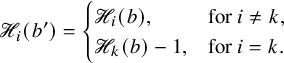 $$ \begin{align} \mathscr{H}_i(b') = \begin{cases} \mathscr{H}_i(b), \qquad &\text{for }i \neq k, \\ \mathscr{H}_k(b)-1, &\text{for }i = k. \end{cases} \end{align} $$
In particular, $\mathscr {H}(b')=\mathscr {H}(b)-1$
.
$\mathscr {H}(b')=\mathscr {H}(b)-1$
.
We give the following natural definition.
Definition 7.8 (Leading map).
For any $b\in B^\varkappa $
, a leading map
$b\in B^\varkappa $
, a leading map $\mathcal {L}_b$
is a composition of Demazure arrows
$\mathcal {L}_b$
is a composition of Demazure arrows $\widetilde {f}_{i}, \widetilde {e}_{i}, i=0,\dots , n-1$
such that
$\widetilde {f}_{i}, \widetilde {e}_{i}, i=0,\dots , n-1$
such that $\mathcal {L}_b (b) = \varkappa ^{\, \mathrm {lv}}$
.
$\mathcal {L}_b (b) = \varkappa ^{\, \mathrm {lv}}$
.
The fact that for any element $b \in B^\varkappa $
a leading map
$b \in B^\varkappa $
a leading map $\mathcal {L}_b$
exists is a consequence of connectedness of the Demazure subgraph stated in Proposition 7.6. Leading maps can be visualized as walks on the Demazure subgraph
$\mathcal {L}_b$
exists is a consequence of connectedness of the Demazure subgraph stated in Proposition 7.6. Leading maps can be visualized as walks on the Demazure subgraph $\widetilde {B}(\varkappa )$
starting at b and terminating at
$\widetilde {B}(\varkappa )$
starting at b and terminating at $\varkappa ^{\mathrm {lv}}$
. For instance, from Figure 18 we see that a leading map for
$\varkappa ^{\mathrm {lv}}$
. For instance, from Figure 18 we see that a leading map for
![]() is given by
is given by
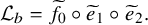 $$ \begin{align} \mathcal{L}_b = \widetilde{f}_{0} \circ \widetilde{e}_{1} \circ \widetilde{e}_{2}. \end{align} $$
Remark 7.9. When there are multiple walks from b to $\varkappa ^{\mathrm {lv}}$
on
$\varkappa ^{\mathrm {lv}}$
on $\widetilde {B}(\varkappa )$
, the leading map
$\widetilde {B}(\varkappa )$
, the leading map $\mathcal {L}_b$
does not admit a unique expansion in terms of Kashiwara operators. However, following the convention on inverse maps established in Section 5.1, given
$\mathcal {L}_b$
does not admit a unique expansion in terms of Kashiwara operators. However, following the convention on inverse maps established in Section 5.1, given $b \in B^{\varkappa }$
and a leading map
$b \in B^{\varkappa }$
and a leading map $\mathcal {L}_b$
it is always true that
$\mathcal {L}_b$
it is always true that $b=\mathcal {L}_b^{-1} (\varkappa ^{\mathrm {lv}})$
.
$b=\mathcal {L}_b^{-1} (\varkappa ^{\mathrm {lv}})$
.
Result of Proposition 7.7 implies that $\mathscr {H}(b)$
is the difference between the number of
$\mathscr {H}(b)$
is the difference between the number of $\widetilde {e}_{0}$
and
$\widetilde {e}_{0}$
and $\widetilde {f}_{0}$
in any leading map
$\widetilde {f}_{0}$
in any leading map $\mathcal {L}_b$
. A more precise version of this statement is given by the next proposition, for which we need to prepare some notation. For any
$\mathcal {L}_b$
. A more precise version of this statement is given by the next proposition, for which we need to prepare some notation. For any $b \in B^\varkappa $
, consider a leading map
$b \in B^\varkappa $
, consider a leading map $\mathcal {L}_b = h_m \circ \cdots \circ h_1$
, where
$\mathcal {L}_b = h_m \circ \cdots \circ h_1$
, where $h_j$
are Demazure arrows. Denote by
$h_j$
are Demazure arrows. Denote by $b^{(j)}=h_j \circ \cdots \circ h_1 (b)$
the partial evaluations of
$b^{(j)}=h_j \circ \cdots \circ h_1 (b)$
the partial evaluations of $\mathcal {L}_b$
for
$\mathcal {L}_b$
for $j=1,\dots ,m$
. Let
$j=1,\dots ,m$
. Let $u_k(\mathcal {L}_b)$
be the number of 0-Demazure arrows
$u_k(\mathcal {L}_b)$
be the number of 0-Demazure arrows $h_j=\widetilde {f}_{0}$
in
$h_j=\widetilde {f}_{0}$
in $\mathcal {L}_b$
such that
$\mathcal {L}_b$
such that
 $$ \begin{align} h_j:b^{(j-1)} \mapsto b_1^{(j-1)} \otimes \cdots \otimes \widetilde{f}_{0}(b_k^{(j-1)}) \otimes \cdots \otimes b_N^{(j-1)}. \end{align} $$
Analogously, define $d_k(\mathcal {L}_b)$
as the number of 0-Demazure arrows
$d_k(\mathcal {L}_b)$
as the number of 0-Demazure arrows $h_j=\widetilde {e}_{0}$
such that
$h_j=\widetilde {e}_{0}$
such that
 $$ \begin{align} h_j:b^{(j-1)} \mapsto b_1^{(j-1)} \otimes \cdots \otimes \widetilde{e}_{0}(b_k^{(j-1)}) \otimes \cdots \otimes b_N^{(j-1)}. \end{align} $$
In other words, $u_k(\mathcal {L}_b)$
(resp.
$u_k(\mathcal {L}_b)$
(resp. $d_k(\mathcal {L}_b)$
) counts the number of
$d_k(\mathcal {L}_b)$
) counts the number of $\widetilde {f}_{0}$
Demazure arrows in
$\widetilde {f}_{0}$
Demazure arrows in $\mathcal {L}_b$
that during the evaluation of
$\mathcal {L}_b$
that during the evaluation of $\mathcal {L}_b$
act as
$\mathcal {L}_b$
act as $\widetilde {f}_{0}$
(resp
$\widetilde {f}_{0}$
(resp $\widetilde {e}_{0}$
) on the k-th tensor factor of the argument. The next proposition relates
$\widetilde {e}_{0}$
) on the k-th tensor factor of the argument. The next proposition relates $u_k$
and
$u_k$
and $d_k$
with the local energy
$d_k$
with the local energy $\mathscr {H}_k$
.
$\mathscr {H}_k$
.
Proposition 7.10. In the notation introduced above, we have
 $$ \begin{align} \mathscr{H}_k(b) = u_k(\mathcal{L}_b) - d_k(\mathcal{L}_b). \end{align} $$
Proof. This follows from Proposition 7.7 and from the fact that $\mathscr {H}_k(\varkappa ^{\mathrm {lv}})=0$
for all k.
$\mathscr {H}_k(\varkappa ^{\mathrm {lv}})=0$
for all k.
One can verify Proposition 7.10 looking at Figure 18. Setting
![]() , local energies can be computed as
, local energies can be computed as
 $$ \begin{align} \mathscr{H}_1(b) = 1, \qquad \mathscr{H}_2(b) = 1, \qquad \mathscr{H}_3(b) = 0, \end{align} $$
either following Proposition 7.4 or checking the action of 0-Demazure arrows throughout any path on the Demazure subgraph connecting b to
![]() .
.
Remark 7.11. It is not true that for any $b\in B^\varkappa $
there always exist a choice of a leading map
$b\in B^\varkappa $
there always exist a choice of a leading map $\mathcal {L}_b$
that does not contain
$\mathcal {L}_b$
that does not contain $\widetilde {e}_{0}$
Demazure arrows. For example, taking
$\widetilde {e}_{0}$
Demazure arrows. For example, taking
one can verify that in the classical connected component of b there does not exist $b'$
such that
$b'$
such that $\varepsilon _0(b')\neq 0$
and
$\varepsilon _0(b')\neq 0$
and $\varphi _0(b') \neq 0$
. Hence in this case
$\varphi _0(b') \neq 0$
. Hence in this case $\mathcal {L}_b$
must contain at least one
$\mathcal {L}_b$
must contain at least one $\widetilde {e}_{0}$
operator.
$\widetilde {e}_{0}$
operator.
Given a pair of vertically strict tableaux $(V,W)$
we define the leading map of the pair
$(V,W)$
we define the leading map of the pair $\mathcal {L}_{V,W}$
as
$\mathcal {L}_{V,W}$
as
 $$ \begin{align} \mathcal{L}_{V,W} : (V',W') \mapsto (\mathcal{L}_V(V') , \mathcal{L}_{W}(W')), \end{align} $$
whenever the operation is defined. Clearly maps $\mathcal {L}_V$
and
$\mathcal {L}_V$
and $\mathcal {L}_W$
are defined through the usual identification of vertically strict tableaux with crystals.
$\mathcal {L}_W$
are defined through the usual identification of vertically strict tableaux with crystals.
7.3 Leading map for pairs of skew tableaux
On the affine bicrystal graph of pairs of skew semistandard tableaux of generalized shape
 $$ \begin{align} \bigcup_{\rho,\lambda} SST(\lambda/\rho,n) \times SST(\lambda/\rho,n), \end{align} $$
we define the Demazure subgraph similarly as in Section 7.2. For either $\epsilon =1,2$
, we say that
$\epsilon =1,2$
, we say that $(P,Q)\to \widetilde {F}^{(\epsilon )}_i(P,Q)$
is a Demazure arrow if
$(P,Q)\to \widetilde {F}^{(\epsilon )}_i(P,Q)$
is a Demazure arrow if $i=1,\dots ,n-1$
or if
$i=1,\dots ,n-1$
or if $i=0$
and
$i=0$
and $\widetilde {E}^{(\epsilon )}_0(P,Q) \neq \varnothing $
. Analogously,
$\widetilde {E}^{(\epsilon )}_0(P,Q) \neq \varnothing $
. Analogously, $(P,Q)\to \widetilde {E}^{(\epsilon )}_i(P,Q)$
is a Demazure arrow if
$(P,Q)\to \widetilde {E}^{(\epsilon )}_i(P,Q)$
is a Demazure arrow if $i=1,\dots ,n-1$
or if
$i=1,\dots ,n-1$
or if $i=0$
and
$i=0$
and $\left (\widetilde {E}^{(\epsilon )}_0\right )^2(P,Q) \neq \varnothing $
.
$\left (\widetilde {E}^{(\epsilon )}_0\right )^2(P,Q) \neq \varnothing $
.
We extend the notion of leading map presented for single vertically strict tableaux in Proposition 7.8 to pairs of semistandard tableaux. This produces a new transformation which, as the other notions related to the affine bicrystal structure of pairs of skew tableaux, is new in this paper.
Definition 7.12 (Leading map for skew tableaux).
Let $P,Q\in SST(\lambda / \rho ,n)$
and consider the projection
$P,Q\in SST(\lambda / \rho ,n)$
and consider the projection $(V,W) = \Phi (P,Q)$
. A leading map for the pair
$(V,W) = \Phi (P,Q)$
. A leading map for the pair $(P,Q)$
, denoted by
$(P,Q)$
, denoted by $\mathcal {L}_{P,Q}$
, is defined as the
$\mathcal {L}_{P,Q}$
, is defined as the $\Phi $
-pullback of a leading map
$\Phi $
-pullback of a leading map $\mathcal {L}_{V,W}$
. In other words, if
$\mathcal {L}_{V,W}$
. In other words, if
 $$ \begin{align*} \mathcal{L}_V= \left(\widetilde{e}_{i_1}\right)^{a_1} \circ \left(\widetilde{f}_{j_1}\right)^{b_1} \!\circ \cdots \circ \left(\widetilde{e}_{i_N}\right)^{a_N} \circ \left(\widetilde{f}_{j_N}\right)^{b_N}\!, \,\,\, \mathcal{L}_W= \left(\widetilde{e}_{k_1}\right)^{c_1} \circ \left(\widetilde{f}_{\ell_1}\right)^{d_1} \circ \cdots \circ \left(\widetilde{e}_{k_M}\right)^{c_M} \circ \left(\widetilde{f}_{\ell_M}\right)^{d_M} \end{align*} $$
are leading maps for V and W, then we define
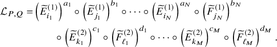 $$ \begin{align} \begin{aligned} \mathcal{L}_{P,Q}=& \left(\widetilde{E}^{(1)}_{i_1}\right)^{a_1} \circ \left(\widetilde{E}^{(1)}_{j_1}\right)^{b_1} \circ \cdots \circ \left(\widetilde{E}^{(1)}_{i_N}\right)^{a_N} \circ \left(\widetilde{F}^{(1)}_{j_N}\right)^{b_N} \\ &\qquad\circ \left(\widetilde{E}^{(2)}_{k_1}\right)^{c_1} \circ \left(\widetilde{F}^{(2)}_{\ell_1}\right)^{d_1} \circ \cdots \circ \left(\widetilde{E}^{(2)}_{k_M}\right)^{c_M} \circ \left(\widetilde{F}^{(2)}_{\ell_M}\right)^{d_M}. \end{aligned} \end{align} $$
We report an example of a leading map for a simple pair of skew tableaux.
Example 7.13. Consider the pair of skew tableaux and the projection
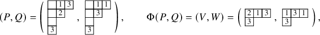
which can be easily computed. A possible leading map for V was computed in (7.16), whereas a leading map for W is given by $\widetilde {e}_{2} \circ \widetilde {f}_{0}$
as it can be seen from Figure 18. This defines the leading map
$\widetilde {e}_{2} \circ \widetilde {f}_{0}$
as it can be seen from Figure 18. This defines the leading map $\mathcal {L}_{P,Q}$
as
$\mathcal {L}_{P,Q}$
as
 $$ \begin{align} \mathcal{L}_{P,Q} = \widetilde{E}^{(2)}_2 \circ \widetilde{F}^{(2)}_0 \circ \widetilde{F}^{(1)}_0 \circ \widetilde{E}^{(1)}_1 \circ \widetilde{E}^{(1)}_2 \end{align} $$
so that
Remark 7.14. As pointed out in Proposition 7.9 a leading map $\mathcal {L}_{P,Q}$
for a pair
$\mathcal {L}_{P,Q}$
for a pair $(P,Q)$
always exists, but its expression in terms of Kashiwara operators is not unique. The nonuniqueness of leading map for a pair
$(P,Q)$
always exists, but its expression in terms of Kashiwara operators is not unique. The nonuniqueness of leading map for a pair $(P,Q)$
might allow, in principle, that the evaluation of two different leading maps
$(P,Q)$
might allow, in principle, that the evaluation of two different leading maps $\mathcal {L}_{P,Q}(P,Q)$
and
$\mathcal {L}_{P,Q}(P,Q)$
and $\mathcal {L}_{P,Q}^{\prime }(P,Q)$
could give different results. This is indeed not the case as proved in Proposition 7.21 below. As a result of this fact, the image
$\mathcal {L}_{P,Q}^{\prime }(P,Q)$
could give different results. This is indeed not the case as proved in Proposition 7.21 below. As a result of this fact, the image $(T,T)$
of any leading map
$(T,T)$
of any leading map $\mathcal {L}_{P,Q}$
does not depend on the realization of
$\mathcal {L}_{P,Q}$
does not depend on the realization of $\mathcal {L}_{P,Q}$
and moreover
$\mathcal {L}_{P,Q}$
and moreover $(P,Q) = \mathcal {L}_{P,Q}^{-1}(T,T)$
. We recall that the convention on inverse maps was discussed in Section 5.1.
$(P,Q) = \mathcal {L}_{P,Q}^{-1}(T,T)$
. We recall that the convention on inverse maps was discussed in Section 5.1.
7.4 Leading tableaux
In this subsection, we aim to characterize the image of a pair $(P,Q)$
of skew tableaux under a leading map
$(P,Q)$
of skew tableaux under a leading map $\mathcal {L}_{P,Q}$
. This result is reported in Proposition 7.21, while its proof is given later in Section 7.5 as it uses the concept of linearization of the skew
$\mathcal {L}_{P,Q}$
. This result is reported in Proposition 7.21, while its proof is given later in Section 7.5 as it uses the concept of linearization of the skew $\mathbf {RSK}$
map discussed in the same section. For our description, we define the following class of tableaux.
$\mathbf {RSK}$
map discussed in the same section. For our description, we define the following class of tableaux.
Definition 7.15 (Leading tableaux).
A semistandard tableau T is leading if, whenever T has $k \ i$
-cells at row r, then it has at least
$k \ i$
-cells at row r, then it has at least $k \ (i-1)$
-cells at row
$k \ (i-1)$
-cells at row $r-1$
for all r and
$r-1$
for all r and $i = 2,3,\dots $
. The content of a leading tableau is hence a partition. We denote the set of leading tableau with classical skew shape and with fixed content
$i = 2,3,\dots $
. The content of a leading tableau is hence a partition. We denote the set of leading tableau with classical skew shape and with fixed content $\mu $
as
$\mu $
as $\mathrm {LdT}(\mu )$
.
$\mathrm {LdT}(\mu )$
.
An example of a leading tableaux is given below in equation (7.43).
Remark 7.16. To keep the notation simple, below we will focus only on the case where $P,Q$
are tableaux of classical skew shape, leaving the case when their shape is a generalized skew Young diagram as an easy exercise.
$P,Q$
are tableaux of classical skew shape, leaving the case when their shape is a generalized skew Young diagram as an easy exercise.
The notion of leading can be translated to matrices, recalling equation (2.17). A matrix $\alpha \in \mathbb {M}_{n,+\infty }$
is called leading when it satisfies
$\alpha \in \mathbb {M}_{n,+\infty }$
is called leading when it satisfies
 $$ \begin{align} \alpha_{1,j} \ge \alpha_{2,j+1} \ge \alpha_{3,j+2} \ge \cdots \qquad \text{for all } j \in \mathbb{N}. \end{align} $$
The set of leading matrices is denoted by $\mathcal {M}^{\mathrm Ld}$
. To get a more explicit description of leading tableaux, we introduce the following notion.
$\mathcal {M}^{\mathrm Ld}$
. To get a more explicit description of leading tableaux, we introduce the following notion.
Definition 7.17. For any partition $\mu $
, define the set
$\mu $
, define the set
 $$ \begin{align}\mathcal{K}(\mu) = \{ (\kappa_1,\dots,\kappa_{\mu_1}) \in \mathbb{N}_0^{\mu_1} : \kappa_i \ge \kappa_{i+1} \text{ if } \mu_i^{\prime} = \mu_{i+1}^{\prime} \}. \end{align} $$
If $0=R_0,R_1,R_2,\dots $
is a rectangular decomposition of
$0=R_0,R_1,R_2,\dots $
is a rectangular decomposition of $\mu $
as defined around equation (2.9), then we will sometimes write elements of
$\mu $
as defined around equation (2.9), then we will sometimes write elements of $\mathcal {K}(\mu )$
as lists of subarrays
$\mathcal {K}(\mu )$
as lists of subarrays $(\kappa ^{(1)},\kappa ^{(2)},\dots )$
, gathering together the weakly decreasing components
$(\kappa ^{(1)},\kappa ^{(2)},\dots )$
, gathering together the weakly decreasing components $\kappa ^{(i)}=(\kappa _{R_{i-1}+1}, \dots \kappa _{R_i})$
. As usual,
$\kappa ^{(i)}=(\kappa _{R_{i-1}+1}, \dots \kappa _{R_i})$
. As usual, $\kappa ^+$
will denote the unique partition that can be formed sorting elements of
$\kappa ^+$
will denote the unique partition that can be formed sorting elements of $\kappa $
and
$\kappa $
and $|\kappa |=\sum _i \kappa _i$
.
$|\kappa |=\sum _i \kappa _i$
.
In the following, we will construct a bijection between $\mathcal {K}(\mu ) \times \mathbb {Y}$
and
$\mathcal {K}(\mu ) \times \mathbb {Y}$
and $\mathrm {LdT}(\mu )$
. This is most conveniently done through row-coordinate matrices. For numbers
$\mathrm {LdT}(\mu )$
. This is most conveniently done through row-coordinate matrices. For numbers $k \in \mathbb {N}_0$
,
$k \in \mathbb {N}_0$
, $m\in \{1,\dots ,n\}$
, define matrices
$m\in \{1,\dots ,n\}$
, define matrices $A(m,k) \in \mathbb {M}_{n,+\infty }$
as
$A(m,k) \in \mathbb {M}_{n,+\infty }$
as
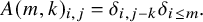 $$ \begin{align} A(m,k)_{i,j} = \delta_{i,j-k} \delta_{i\le m}. \end{align} $$
That is, $A(m,k)$
’s only nonzero values are the first m entries in the
$A(m,k)$
’s only nonzero values are the first m entries in the $(k+1)$
-th upper diagonal
$(k+1)$
-th upper diagonal $A(m,k)_{1,k+1} = \cdots = A(m,k)_{m,k+m} = 1$
. For a given
$A(m,k)_{1,k+1} = \cdots = A(m,k)_{m,k+m} = 1$
. For a given $\kappa \in \mathcal {K}(\mu )$
, construct a matrix
$\kappa \in \mathcal {K}(\mu )$
, construct a matrix
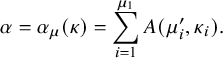 $$ \begin{align}\alpha = \alpha_{\mu}(\kappa)=\sum_{i=1}^{\mu_1} A(\mu_i^{\prime}, \kappa_i). \end{align} $$
This is obviously leading, but in fact the opposite is also true as stated in the next proposition. For a given $\mu $
, let us denote by
$\mu $
, let us denote by $\mathcal {M}^{\mathrm Ld}(\mu )$
the set of leading matrices
$\mathcal {M}^{\mathrm Ld}(\mu )$
the set of leading matrices $\alpha $
such that
$\alpha $
such that $\alpha _{i,1}+\alpha _{i,2}+\cdots =\mu _i$
for all i. In other words,
$\alpha _{i,1}+\alpha _{i,2}+\cdots =\mu _i$
for all i. In other words, $\mathcal {M}^{\mathrm Ld}(\mu )$
represents the set of row-coordinate matrices of leading tableaux T with content
$\mathcal {M}^{\mathrm Ld}(\mu )$
represents the set of row-coordinate matrices of leading tableaux T with content $\gamma (T)=\mu $
. Then we have the following.
$\gamma (T)=\mu $
. Then we have the following.
Proposition 7.18. For a given $\mu $
, the map
$\mu $
, the map $\alpha _{\mu }$
defined in equation (7.31) is a bijection between
$\alpha _{\mu }$
defined in equation (7.31) is a bijection between $\mathcal {K}(\mu )$
and
$\mathcal {K}(\mu )$
and $\mathcal {M}^{\mathrm Ld}(\mu )$
.
$\mathcal {M}^{\mathrm Ld}(\mu )$
.
Proof. We will indeed establish the bijection between the set $\{ (\mu ,\kappa ),\mu \in \mathbb {Y}, \kappa \in \mathcal {K}(\mu )\}$
and
$\{ (\mu ,\kappa ),\mu \in \mathbb {Y}, \kappa \in \mathcal {K}(\mu )\}$
and $\mathcal {M}^{\mathrm Ld}$
. Restriction to a fixed
$\mathcal {M}^{\mathrm Ld}$
. Restriction to a fixed $\mu $
gives the bijection in the statement of the lemma. We only have to show that any leading matrix
$\mu $
gives the bijection in the statement of the lemma. We only have to show that any leading matrix $\alpha \in \mathbb {M}_{n,+\infty }$
can be uniquely written in the form of equation (7.31). We peel off matrix
$\alpha \in \mathbb {M}_{n,+\infty }$
can be uniquely written in the form of equation (7.31). We peel off matrix $\alpha $
with the help of the
$\alpha $
with the help of the $A(m,k)$
’s removing maximal diagonals of nonzero entries. Define numbers
$A(m,k)$
’s removing maximal diagonals of nonzero entries. Define numbers $k_1,m_1$
as
$k_1,m_1$
as
 $$ \begin{align} k_1=\min \{ k : \alpha_{1,k+1}> 0 \}, \qquad \qquad m_1 = \max\{ m : \alpha_{m,k_1 + m} >0 \} \end{align} $$
and let
 $$ \begin{align} \alpha^{(1)} = \alpha - A(m_1,k_1). \end{align} $$
Then, by equation (7.28) and by the fact that $m_1$
is maximal, also
$m_1$
is maximal, also $\alpha ^{(1)}$
is a leading matrix. We can now recursively construct
$\alpha ^{(1)}$
is a leading matrix. We can now recursively construct
 $$ \begin{align} k_j = \min \{ k : \alpha^{(j-1)}_{1,k+1}> 0 \}, \qquad m_j = \max\{ m : \alpha^{(j-1)}_{m,k_j + m} >0 \} \end{align} $$
and $\alpha ^{(j)} = \alpha ^{(j-1)} - A(m_j,k_j)$
, until for some
$\alpha ^{(j)} = \alpha ^{(j-1)} - A(m_j,k_j)$
, until for some $j'$
we exhaust all positive entries and
$j'$
we exhaust all positive entries and $\alpha ^{(j')}=0$
. This proves that there exist
$\alpha ^{(j')}=0$
. This proves that there exist $k_1,k_2,\dots $
and
$k_1,k_2,\dots $
and $m_1,m_2,\dots $
such that
$m_1,m_2,\dots $
such that
 $$ \begin{align} \alpha = A(m_1,k_1) + A(m_2,k_2) + \cdots. \end{align} $$
It is clear that $\mu _i^{\prime } = m_{j_i}$
for some
$\mu _i^{\prime } = m_{j_i}$
for some $j_1, j_2, \cdots $
. To avoid ambiguity, we choose
$j_1, j_2, \cdots $
. To avoid ambiguity, we choose $j_i$
such that
$j_i$
such that $k_{j_i}> k_{j_{i+1}}$
whenever
$k_{j_i}> k_{j_{i+1}}$
whenever $\mu _i^{\prime } = \mu _{i+1}^{\prime }$
. Defining the new sequence
$\mu _i^{\prime } = \mu _{i+1}^{\prime }$
. Defining the new sequence $\tilde {k}_1 = k_{j_1}, \tilde {k}_2 = k_{j_2} , \dots $
, we can finally identify
$\tilde {k}_1 = k_{j_1}, \tilde {k}_2 = k_{j_2} , \dots $
, we can finally identify $\kappa =(\kappa ^{(1)},\kappa ^{(2)}, \dots )$
as
$\kappa =(\kappa ^{(1)},\kappa ^{(2)}, \dots )$
as
 $$ \begin{align} \kappa^{(i)} = ( \tilde{k}_{R_{i-1}+1}, \dots , \tilde{k}_{R_i} ). \end{align} $$
As we mentioned below, Proposition 2.4, there is a bijection
![]() between a pair
between a pair $(\alpha ,\nu )$
of a row-coordinate matrix
$(\alpha ,\nu )$
of a row-coordinate matrix $\alpha $
and a partition
$\alpha $
and a partition $\nu $
, and a classical tableau P. Restriction to leading ones gives a bijection between
$\nu $
, and a classical tableau P. Restriction to leading ones gives a bijection between $\mathcal {M}^{\mathrm Ld}(\mu )\times \mathbb {Y}$
and
$\mathcal {M}^{\mathrm Ld}(\mu )\times \mathbb {Y}$
and $\mathrm {LdT}(\mu )$
. Combining this with the bijection between
$\mathrm {LdT}(\mu )$
. Combining this with the bijection between $\mathcal {K}(\mu )$
and
$\mathcal {K}(\mu )$
and $\mathcal {M}^{\mathrm Ld}(\mu )$
in Proposition 7.18, we get the desired characterization of the set of leading tableaux.
$\mathcal {M}^{\mathrm Ld}(\mu )$
in Proposition 7.18, we get the desired characterization of the set of leading tableaux.
Proposition 7.19. For a given $\mu \in \mathbb {Y}$
, the map
$\mu \in \mathbb {Y}$
, the map
 $$ \begin{align} T(\mu, \cdot; \cdot) :\mathcal{K}(\mu) \times \mathbb{Y} \longrightarrow \mathrm{LdT}(\mu), \end{align} $$
defined by
where $\kappa \in \mathcal {K}(\mu ), \nu \in \mathbb {Y}$
, is a bijection. Moreover, if
$\kappa \in \mathcal {K}(\mu ), \nu \in \mathbb {Y}$
, is a bijection. Moreover, if $\lambda /\rho $
is the shape of
$\lambda /\rho $
is the shape of $T(\mu ,\kappa ;\nu )$
, then
$T(\mu ,\kappa ;\nu )$
, then $\rho = (\kappa ^+)' + \nu $
.
$\rho = (\kappa ^+)' + \nu $
.
Proof. The first part has already been shown in the arguments above. We are left to check that $(\kappa ,\nu ) \mapsto T(\mu ,\kappa ;\nu )$
satisfies relation
$(\kappa ,\nu ) \mapsto T(\mu ,\kappa ;\nu )$
satisfies relation $\rho =(\kappa ^+)' + \nu $
. By the fact that
$\rho =(\kappa ^+)' + \nu $
. By the fact that $\nu = \ker (T(\mu ,\kappa ;\nu )) $
, we only need to show that such property holds for
$\nu = \ker (T(\mu ,\kappa ;\nu )) $
, we only need to show that such property holds for $\nu =\varnothing $
. For this notice that if
$\nu =\varnothing $
. For this notice that if $p^{(1)},p^{(2)},\dots $
are the first, second, …row words of
$p^{(1)},p^{(2)},\dots $
are the first, second, …row words of $T=T(\mu ,\kappa ;\varnothing )$
, then, since T is leading, we have
$T=T(\mu ,\kappa ;\varnothing )$
, then, since T is leading, we have
 $$ \begin{align} \mathrm{ov}(p^{(j+1)},p^{(j)}) = \ell( p^{(j+1)} ) - m_1(p^{(j+1)}), \end{align} $$
where $\ell , m_1$
denote, respectively, the length and the multiplicity of letter
$\ell , m_1$
denote, respectively, the length and the multiplicity of letter $1$
in the word
$1$
in the word $p^{(j+1)}$
. Calling
$p^{(j+1)}$
. Calling $\eta $
the empty shape of T, we have, by equation (2.22)
$\eta $
the empty shape of T, we have, by equation (2.22)
 $$ \begin{align} \eta_j - \eta_{j+1} = m_1 (p^{(j+1)}). \end{align} $$
This implies that $\eta = (\kappa ^+)'$
.
$\eta = (\kappa ^+)'$
.
Example 7.20. First, let us construct a leading tableaux for a given triple $\mu ,\kappa ,\nu $
. Consider the case
$\mu ,\kappa ,\nu $
. Consider the case $\mu =(4, 2 , 2, 1), \kappa = ((1),(3),(2,1)), \nu = (1,1)$
and for the sake of a better visualization we present these quantities in a colored form as
$\mu =(4, 2 , 2, 1), \kappa = ((1),(3),(2,1)), \nu = (1,1)$
and for the sake of a better visualization we present these quantities in a colored form as
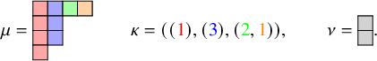
Then we determine, using equation (7.37), the row-coordinate matrix $\alpha $
as
$\alpha $
as
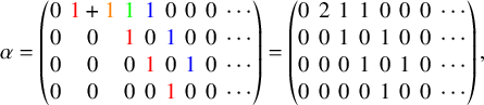
resulting in the tableau
![]()
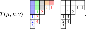
One can also check that the procedure can be reversed to recover $\mu ,\kappa ,\nu $
from the leading tableau above.
$\mu ,\kappa ,\nu $
from the leading tableau above.
Before ending the subsection, we state a result for the image of $(P,Q)$
under a leading map
$(P,Q)$
under a leading map $\mathcal {L}$
.
$\mathcal {L}$
.
Theorem 7.21. Let $P,Q \in SST(\lambda / \rho ,n)$
, for
$P,Q \in SST(\lambda / \rho ,n)$
, for $\lambda ,\rho \in \mathbb {Y}$
. Then for any leading map
$\lambda ,\rho \in \mathbb {Y}$
. Then for any leading map $\mathcal {L}_{P,Q}$
we have
$\mathcal {L}_{P,Q}$
we have $(T,T)=\mathcal {L}_{P,Q}(P,Q)$
, where T is a leading tableau independent of the particular choice of
$(T,T)=\mathcal {L}_{P,Q}(P,Q)$
, where T is a leading tableau independent of the particular choice of $\mathcal {L}_{P,Q}$
. Moreover,
$\mathcal {L}_{P,Q}$
. Moreover, $T\in \mathrm {LdT}(\mu )$
, where
$T\in \mathrm {LdT}(\mu )$
, where $\mu $
is the Greene invariant corresponding to
$\mu $
is the Greene invariant corresponding to $P,Q$
.
$P,Q$
.
A proof of this theorem will be given in the next subsection because it uses a linearization of the skew $\mathbf {RSK}$
map for leading tableaux which is explained below.
$\mathbf {RSK}$
map for leading tableaux which is explained below.
7.5 Linearization
The property of being leading for a tableau is preserved by the skew $\mathbf {RSK}$
map. Moreover, the action of the skew
$\mathbf {RSK}$
map. Moreover, the action of the skew $\mathbf {RSK}$
map on leading tableaux reduces to a simple shift of
$\mathbf {RSK}$
map on leading tableaux reduces to a simple shift of $\kappa $
by
$\kappa $
by $\mu '$
. This is the main result we state and prove in this subsection.
$\mu '$
. This is the main result we state and prove in this subsection.
Theorem 7.22 (Skew
$\mathbf {RSK}$
map on leading tableaux).

Let $T=T(\mu ,\kappa ;\nu )\in \mathrm {LdT}(\mu )$
and
$T=T(\mu ,\kappa ;\nu )\in \mathrm {LdT}(\mu )$
and $(T',T')=\mathbf {RSK}(T,T)$
. Then
$(T',T')=\mathbf {RSK}(T,T)$
. Then $T'$
is also a leading tableau and we have
$T'$
is also a leading tableau and we have $T'=T(\mu ,\kappa + \mu ';\nu )$
.
$T'=T(\mu ,\kappa + \mu ';\nu )$
.
The proof of Proposition 7.22 is based on a direct inspection of the skew $\mathbf {RSK}$
map on a pair
$\mathbf {RSK}$
map on a pair $(T,T)$
, for a leading tableau T. We will need the following preliminary result.
$(T,T)$
, for a leading tableau T. We will need the following preliminary result.
Lemma 7.23. Fix a weakly decreasing array
![]() . Let
. Let
![]() be a subarray of
be a subarray of
![]() with
with
![]() for
for $j_1> \cdots > j_M$
. Consider the skew
$j_1> \cdots > j_M$
. Consider the skew $\mathbf {RS}$
map
$\mathbf {RS}$
map
![]() . Then we have
. Then we have
and there exists indices $J'=\{j_1^{\prime }, \dots ,j_M^{\prime }\}$
such that
$J'=\{j_1^{\prime }, \dots ,j_M^{\prime }\}$
such that
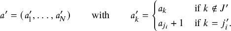
Proof. Define index $j_1^{\prime }$
as the position of the leftmost element of
$j_1^{\prime }$
as the position of the leftmost element of
equal to
and then, sequentially define
. Since
is a subarray of
and
is weakly decreasing indices $j_1^{\prime },\dots , j_M^{\prime }$
exist. To compute the skew
$j_1^{\prime },\dots , j_M^{\prime }$
exist. To compute the skew $\mathbf {RS}$
map of
$\mathbf {RS}$
map of
and
, we produce the edge configuration in the rectangle $\{1,\dots ,N \} \times \{1 ,\dots , M \}$
with boundary data
$\{1,\dots ,N \} \times \{1 ,\dots , M \}$
with boundary data
Consider the edge configuration along the bottom row of the rectangle. From local rules (3.12) and from the fact that
is weakly decreasing, it is clear that
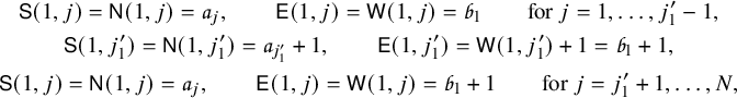
where in the second line we used the fact that
; see Figure 19. Moreover, by definition of index $j_1^{\prime }$
the array
$j_1^{\prime }$
the array
is still weakly decreasing. We now move on with the evaluation of the edge configuration along the second row of the rectangle. Just as for the first row case, we have
The skew $\mathbf {RS}$
map of a weakly decreasing array
$\mathbf {RS}$
map of a weakly decreasing array
![]() with an element
with an element
![]() .
.
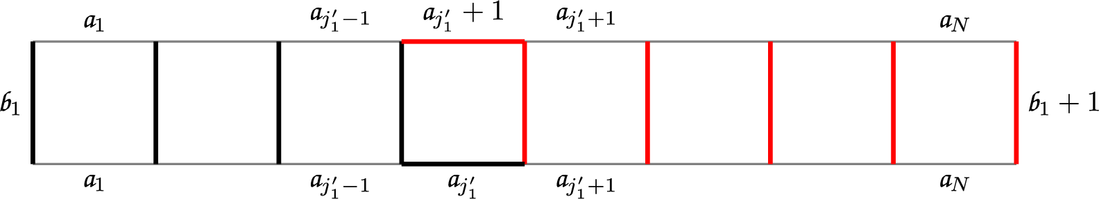

Repeating the same argument M times yields the proof.
Proof of Proposition 7.22.
We know, by Proposition 3.8, that if $\nu =\ker (T)=\ker (T,T)$
, then
$\nu =\ker (T)=\ker (T,T)$
, then $\nu =\ker (T')=\ker (T',T')$
, so we reduce to prove our statement in the case
$\nu =\ker (T')=\ker (T',T')$
, so we reduce to prove our statement in the case $\nu = \varnothing $
. Let
$\nu = \varnothing $
. Let $\alpha =\mathrm {rc}(T)$
. To prove our claim we need to compute
$\alpha =\mathrm {rc}(T)$
. To prove our claim we need to compute $(\alpha ',\alpha ')=\mathbf {RSK}(\alpha ,\alpha )$
. We use, as usual, standardization and we encode matrix
$(\alpha ',\alpha ')=\mathbf {RSK}(\alpha ,\alpha )$
. We use, as usual, standardization and we encode matrix $\alpha $
, in an array
$\alpha $
, in an array
with $M_i= \mu _1 + \dots + \mu _i$
. Subarrays
$M_i= \mu _1 + \dots + \mu _i$
. Subarrays
![]() record row coordinates of i-cells of T and are weakly decreasing
record row coordinates of i-cells of T and are weakly decreasing
![]() . The leading property of T implies that
. The leading property of T implies that
for $i,r \ge 1$
, where again
$i,r \ge 1$
, where again $m_r$
is the multiplicity of letter r in a word. Moreover, by equation (7.37) we have that, as sets
$m_r$
is the multiplicity of letter r in a word. Moreover, by equation (7.37) we have that, as sets
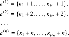
Let now
![]() be the array encoding row coordinates of cells of
be the array encoding row coordinates of cells of $T'$
. Or in other words, let
$T'$
. Or in other words, let
![]() . Then statement of Proposition 7.22 reduces to show that, as sets
. Then statement of Proposition 7.22 reduces to show that, as sets
We prove equation (7.50) by an induction argument over n. When $n=1$
we have
$n=1$
we have
![]() and by Proposition 7.23
and by Proposition 7.23
![]() is obtained by adding one to each entry of
is obtained by adding one to each entry of
![]() .
.
Consider now the array
![]() , and assume, by induction that our theorem holds for any array of
, and assume, by induction that our theorem holds for any array of $(n-1)$
maximal nonincreasing components. In particular, define
$(n-1)$
maximal nonincreasing components. In particular, define
By inductive hypothesis, we have that, as sets
By definition of skew $\mathbf {RS}$
map, depicted in Figure 20, it is clear that
$\mathbf {RS}$
map, depicted in Figure 20, it is clear that
Computation of
![]() by induction over subarrays
by induction over subarrays
![]()
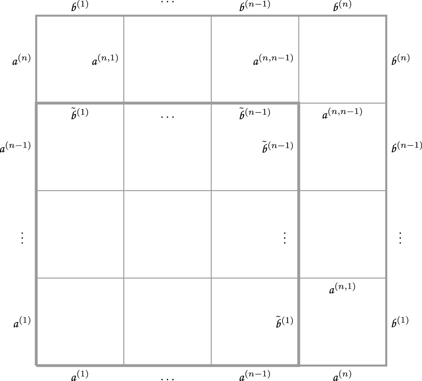
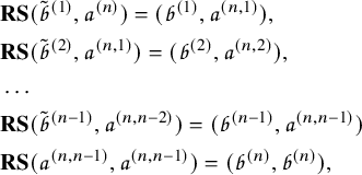
for arrays
![]() and we use these relations to evaluate
and we use these relations to evaluate
![]() . We start with
. We start with
![]() . Since
. Since
and
we can apply Proposition 7.23 to discover that
and
which confirms equation (7.50) for $i=1$
. We can then move to the computation of
$i=1$
. We can then move to the computation of
![]() . We have
. We have
so that again, by Proposition 7.23, taking the skew $\mathbf {RS}$
map of
$\mathbf {RS}$
map of
![]() and
and
![]() we find that
we find that
and
confirming equation (7.50) for $i=2$
. It is clear that we can iterate the same argument for any
$i=2$
. It is clear that we can iterate the same argument for any $i=1,\dots ,n-1$
repeatedly using Proposition 7.23 and obtaining
$i=1,\dots ,n-1$
repeatedly using Proposition 7.23 and obtaining
confirming equation (7.50) for all cases except $i=n$
. To verify this final case, we can easily see, either by direct inspection or through Proposition 7.23, that
$i=n$
. To verify this final case, we can easily see, either by direct inspection or through Proposition 7.23, that
yields the predicted result (7.50). This completes the proof.
An application of Proposition 7.22 gives a proof of Proposition 7.21, presented below. We need the following technical lemma stating that 0-Demazure arrows fix the space of pairs of skew tableau with classical shape.
Lemma 7.24. Let $(P,Q)$
be a pair of skew tableaux with same shape
$(P,Q)$
be a pair of skew tableaux with same shape $\lambda / \rho $
with
$\lambda / \rho $
with $\lambda ,\rho \in \mathbb {Y}$
. Define
$\lambda ,\rho \in \mathbb {Y}$
. Define $(\widetilde {P},\widetilde {Q})=h(P,Q)\neq \varnothing $
for
$(\widetilde {P},\widetilde {Q})=h(P,Q)\neq \varnothing $
for $h\in \{\widetilde {E}_0^{(1)},\widetilde {E}_0^{(2)},\widetilde {F}_0^{(1)},\widetilde {F}_0^{(2)} \}$
such that h is a 0-Demazure arrow. Then, denoting denoting by
$h\in \{\widetilde {E}_0^{(1)},\widetilde {E}_0^{(2)},\widetilde {F}_0^{(1)},\widetilde {F}_0^{(2)} \}$
such that h is a 0-Demazure arrow. Then, denoting denoting by $\widetilde {\lambda } / \widetilde {\rho }$
the shape of
$\widetilde {\lambda } / \widetilde {\rho }$
the shape of $\widetilde {P},\widetilde {Q}$
, we have
$\widetilde {P},\widetilde {Q}$
, we have $\widetilde {\lambda }, \widetilde {\rho } \in \mathbb {Y}$
, or in other words all cells of
$\widetilde {\lambda }, \widetilde {\rho } \in \mathbb {Y}$
, or in other words all cells of $\widetilde {P},\widetilde {Q}$
lie at positive rows.
$\widetilde {P},\widetilde {Q}$
lie at positive rows.
Proof. We prove our statement only for h being a 0-Demazure arrow $\widetilde {E}_0^{(1)}$
or
$\widetilde {E}_0^{(1)}$
or $\widetilde {F}_0^{(1)}$
, as the complementary cases are analogous. We focus first on the case
$\widetilde {F}_0^{(1)}$
, as the complementary cases are analogous. We focus first on the case $h=\widetilde {F}^{(1)}_0 (=\iota _1 \circ (\tilde {f}_1\times 1) \circ \iota _1^{-1})$
. Let
$h=\widetilde {F}^{(1)}_0 (=\iota _1 \circ (\tilde {f}_1\times 1) \circ \iota _1^{-1})$
. Let $(\widehat {P},\widehat {Q})=\iota _1^{-1}(P,Q)$
, and let
$(\widehat {P},\widehat {Q})=\iota _1^{-1}(P,Q)$
, and let $\widehat {\pi }$
be the column reading word of
$\widehat {\pi }$
be the column reading word of $\widehat {P}$
. Then, by definition of 0-Demazure arrow we have
$\widehat {P}$
. Then, by definition of 0-Demazure arrow we have $\widetilde {e}_{1}(\widehat {\pi }), \widetilde {f}_{1}(\widehat {\pi })\neq \varnothing $
and we want to understand implications of this fact. As in the signature rule (5.3) we assign parentheses ‘)’ and ‘(’, respectively, to each occurrence of a 1 and of a 2 letter in
$\widetilde {e}_{1}(\widehat {\pi }), \widetilde {f}_{1}(\widehat {\pi })\neq \varnothing $
and we want to understand implications of this fact. As in the signature rule (5.3) we assign parentheses ‘)’ and ‘(’, respectively, to each occurrence of a 1 and of a 2 letter in $\widehat {\pi }$
. Then, matching consecutive pairs of opening and closing unmatched parentheses we reach a reduced word
$\widehat {\pi }$
. Then, matching consecutive pairs of opening and closing unmatched parentheses we reach a reduced word $)^{\varphi _1(\widehat {\pi })} (^{\varepsilon _1(\widehat {\pi })}$
with
$)^{\varphi _1(\widehat {\pi })} (^{\varepsilon _1(\widehat {\pi })}$
with $\varphi _1(\widehat {\pi }), \varepsilon _1(\widehat {\pi })>0$
. Each of these unmatched ‘)’ parentheses identifies a different 1 letter in
$\varphi _1(\widehat {\pi }), \varepsilon _1(\widehat {\pi })>0$
. Each of these unmatched ‘)’ parentheses identifies a different 1 letter in $\widehat {\pi }$
, which unambiguously identify a 1-cell in
$\widehat {\pi }$
, which unambiguously identify a 1-cell in $\widehat {P}$
. Call
$\widehat {P}$
. Call $\theta _1$
the set of
$\theta _1$
the set of $\varphi _1(\widehat {\pi })$
such 1-cells in
$\varphi _1(\widehat {\pi })$
such 1-cells in $\widehat {P}$
. Analogously, call
$\widehat {P}$
. Analogously, call $\theta _2$
the set of 2-cells of
$\theta _2$
the set of 2-cells of $\widehat {P}$
corresponding to the
$\widehat {P}$
corresponding to the $\varepsilon _1(\widehat {\pi })$
unmatched ‘(’ parentheses in the reduced word generated from
$\varepsilon _1(\widehat {\pi })$
unmatched ‘(’ parentheses in the reduced word generated from $\widehat {\pi }$
. By the definition of the matching procedure, it is clear that each cell of
$\widehat {\pi }$
. By the definition of the matching procedure, it is clear that each cell of $\theta _1$
lies at a column strictly to the left of any cell of
$\theta _1$
lies at a column strictly to the left of any cell of $\theta _2$
. In particular, no cell of
$\theta _2$
. In particular, no cell of $\theta _1$
occupies the rightmost column of
$\theta _1$
occupies the rightmost column of $\widehat {P}$
. Since the application of
$\widehat {P}$
. Since the application of $\widetilde {f}_{1}:\widehat {P} \mapsto \widetilde {f}_{1}(\widehat {P})$
changes the label of a cell of
$\widetilde {f}_{1}:\widehat {P} \mapsto \widetilde {f}_{1}(\widehat {P})$
changes the label of a cell of $\theta _1$
from
$\theta _1$
from $1\mapsto 2$
, it is clear that
$1\mapsto 2$
, it is clear that $\widetilde {F}^{(1)}_0(P,Q)$
cannot modify the rightmost column of
$\widetilde {F}^{(1)}_0(P,Q)$
cannot modify the rightmost column of $P,Q$
. This clearly also implies that every cell of tableaux
$P,Q$
. This clearly also implies that every cell of tableaux $\widetilde {F}^{(1)}_0(P,Q)$
lies at positive rows since so does every cell of their rightmost columns.
$\widetilde {F}^{(1)}_0(P,Q)$
lies at positive rows since so does every cell of their rightmost columns.
When $h=\widetilde {E}_0^{(1)}$
, we have that both
$h=\widetilde {E}_0^{(1)}$
, we have that both $\widetilde {e}_{1}(\widehat {P}),\widetilde {e}_{1}^{\,2}(\widehat {P})\neq \varnothing $
and also in this case, using signature rule as explained above, operator
$\widetilde {e}_{1}(\widehat {P}),\widetilde {e}_{1}^{\,2}(\widehat {P})\neq \varnothing $
and also in this case, using signature rule as explained above, operator $\widetilde {e}_{1}$
cannot transform any 2-cell lying at the rightmost column of
$\widetilde {e}_{1}$
cannot transform any 2-cell lying at the rightmost column of $\widehat {P}$
. This completes the proof.
$\widehat {P}$
. This completes the proof.
Proof of Proposition 7.21.
By Proposition 5.7 any $\mathcal {L}_{P,Q}$
commutes with the skew
$\mathcal {L}_{P,Q}$
commutes with the skew $\mathbf {RSK}$
map. We can therefore write, for any t,
$\mathbf {RSK}$
map. We can therefore write, for any t,
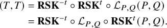 $$ \begin{align} \begin{aligned} (T,T) &= \mathbf{RSK}^{-t} \circ \mathbf{RSK}^t \circ \mathcal{L}_{P,Q}(P,Q) \\ &= \mathbf{RSK}^{-t} \circ \mathcal{L}_{P,Q} \circ \mathbf{RSK}^t (P,Q). \end{aligned} \end{align} $$
Let $(\widetilde {P},\widetilde {Q}) = \mathbf {RSK}^t (P,Q)$
. It is clear that
$(\widetilde {P},\widetilde {Q}) = \mathbf {RSK}^t (P,Q)$
. It is clear that $\mathcal {L}_{P,Q}$
is a leading map also for
$\mathcal {L}_{P,Q}$
is a leading map also for $(\widetilde {P},\widetilde {Q})$
since
$(\widetilde {P},\widetilde {Q})$
since $\Phi (P,Q)=\Phi (\widetilde {P},\widetilde {Q})$
. When t is large, the pair
$\Phi (P,Q)=\Phi (\widetilde {P},\widetilde {Q})$
. When t is large, the pair $(\widetilde {P},\widetilde {Q})$
becomes
$(\widetilde {P},\widetilde {Q})$
becomes $\mathbf {RSK}$
-stable. In such cases, the action of the leading map
$\mathbf {RSK}$
-stable. In such cases, the action of the leading map $\mathcal {L}_{P,Q}$
deforms the original shape of
$\mathcal {L}_{P,Q}$
deforms the original shape of $\widetilde {P},\widetilde {Q}$
as prescribed by Proposition 5.12, but it does not change the number of labeled cells lying at each column. Therefore,
$\widetilde {P},\widetilde {Q}$
as prescribed by Proposition 5.12, but it does not change the number of labeled cells lying at each column. Therefore, $(\widetilde {T},\widetilde {T}) = \mathcal {L}_{P,Q}(\widetilde {P},\widetilde {Q})$
clearly defines a leading tableau
$(\widetilde {T},\widetilde {T}) = \mathcal {L}_{P,Q}(\widetilde {P},\widetilde {Q})$
clearly defines a leading tableau $\widetilde {T}$
. This is because labeled cells at the i-th column of
$\widetilde {T}$
. This is because labeled cells at the i-th column of $\widetilde {T}$
are exactly
$\widetilde {T}$
are exactly $(\mu _i^{\prime })^{\mathrm {lv}}$
. By Proposition 7.19, we write
$(\mu _i^{\prime })^{\mathrm {lv}}$
. By Proposition 7.19, we write $\widetilde {T}=T(\mu , \widetilde {\kappa };\nu )$
, for some uniquely determined
$\widetilde {T}=T(\mu , \widetilde {\kappa };\nu )$
, for some uniquely determined $\widetilde {\kappa },\nu $
. We want to show that
$\widetilde {\kappa },\nu $
. We want to show that $\widetilde {\kappa },\nu $
are independent of the choice of leading map
$\widetilde {\kappa },\nu $
are independent of the choice of leading map $\mathcal {L}_{P,Q}$
and subsequently derive that T is a leading tableau with
$\mathcal {L}_{P,Q}$
and subsequently derive that T is a leading tableau with $T=T(\mu ,\kappa ;\nu )$
where, by Proposition 7.22, we have
$T=T(\mu ,\kappa ;\nu )$
where, by Proposition 7.22, we have
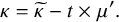 $$ \begin{align} \kappa = \widetilde{\kappa} - t \times \mu'. \end{align} $$
This will imply that tableaux T is independent of the particular choice of $\mathcal {L}_{P,Q}$
yielding the proof.
$\mathcal {L}_{P,Q}$
yielding the proof.
We first observe that partition $\nu $
is independent of
$\nu $
is independent of $\mathcal {L}_{P,Q}$
since
$\mathcal {L}_{P,Q}$
since $\nu =\ker (\widetilde {T})=\ker (\widetilde {P},\widetilde {Q})$
. The second equality follows from the general fact that Kashiwara operators
$\nu =\ker (\widetilde {T})=\ker (\widetilde {P},\widetilde {Q})$
. The second equality follows from the general fact that Kashiwara operators $\widetilde {E}^{(\epsilon )}_i,\widetilde {F}^{(\epsilon )}_i$
preserve the kernel of any pair of tableaux as implied by Proposition 3.8. To prove independence of
$\widetilde {E}^{(\epsilon )}_i,\widetilde {F}^{(\epsilon )}_i$
preserve the kernel of any pair of tableaux as implied by Proposition 3.8. To prove independence of $\widetilde {\kappa }$
from
$\widetilde {\kappa }$
from $\mathcal {L}_{P,Q}$
, we combine Proposition 5.12 and Proposition 7.10. Let
$\mathcal {L}_{P,Q}$
, we combine Proposition 5.12 and Proposition 7.10. Let $\widetilde {\lambda }/\widetilde {\rho }$
be the skew shape of
$\widetilde {\lambda }/\widetilde {\rho }$
be the skew shape of $(\widetilde {P},\widetilde {Q})$
, and denote by
$(\widetilde {P},\widetilde {Q})$
, and denote by $\widehat {\lambda }/ \widehat {\rho }$
the skew shape of
$\widehat {\lambda }/ \widehat {\rho }$
the skew shape of $\widetilde {T}$
. As observed above, any leading map
$\widetilde {T}$
. As observed above, any leading map $\mathcal {L}_{P,Q}$
in addition to modifying the content of
$\mathcal {L}_{P,Q}$
in addition to modifying the content of $\widetilde {P},\widetilde {Q}$
can only shift columns rigidly upward or downward. By Proposition 7.10, we can quantify by how many cells each column gets displaced. Calling
$\widetilde {P},\widetilde {Q}$
can only shift columns rigidly upward or downward. By Proposition 7.10, we can quantify by how many cells each column gets displaced. Calling $(V,W)=\Phi (P,Q)$
and assuming
$(V,W)=\Phi (P,Q)$
and assuming $\mathcal {L}_{P,Q}$
is the
$\mathcal {L}_{P,Q}$
is the $\Phi $
-pullback of the leading map
$\Phi $
-pullback of the leading map $\mathcal {L}_{V,W}$
, we have
$\mathcal {L}_{V,W}$
, we have
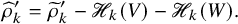 $$ \begin{align} \widehat{\rho}_k^{\prime} = \widetilde{\rho}_k^{\prime} - \mathscr{H}_k(V) - \mathscr{H}_k(W). \end{align} $$
Such expression for $\widehat {\rho }'$
is independent of
$\widehat {\rho }'$
is independent of $\mathcal {L}_{P,Q}$
. By Proposition 7.19,
$\mathcal {L}_{P,Q}$
. By Proposition 7.19, $\widetilde {\kappa }$
is also independent of
$\widetilde {\kappa }$
is also independent of $\mathcal {L}_{P,Q}$
since it is determined by
$\mathcal {L}_{P,Q}$
since it is determined by $\widehat {\rho } = (\widetilde {\kappa }^+)' +\nu $
.
$\widehat {\rho } = (\widetilde {\kappa }^+)' +\nu $
.
In order to complete the proof, we want to check that $\kappa $
, defined by equation (7.64), does in fact belong to
$\kappa $
, defined by equation (7.64), does in fact belong to $\mathcal {K}(\mu )$
. Since
$\mathcal {K}(\mu )$
. Since $\kappa _k = \widetilde {\kappa }_k - t \mu _k^{\prime }$
, it is clear that, recalling the notation of Proposition 7.17,
$\kappa _k = \widetilde {\kappa }_k - t \mu _k^{\prime }$
, it is clear that, recalling the notation of Proposition 7.17, $\kappa ^{(i)}_1 \ge \kappa ^{(i)}_2 \ge \cdots $
for all
$\kappa ^{(i)}_1 \ge \kappa ^{(i)}_2 \ge \cdots $
for all $i=1,2,\dots $
, so we only need to verify that
$i=1,2,\dots $
, so we only need to verify that $\kappa ^{(i)}_k\ge 0$
for all i and k. The last statement holds if tableau T does not have cells at nonpositive rows, condition that is guaranteed by Proposition 7.24. This concludes the proof.
$\kappa ^{(i)}_k\ge 0$
for all i and k. The last statement holds if tableau T does not have cells at nonpositive rows, condition that is guaranteed by Proposition 7.24. This concludes the proof.
8 A new bijection
In this section, we establish a bijection between a pair of skew tableaux $(P,Q)$
and a quadruple
$(P,Q)$
and a quadruple $(V,W;\kappa ;\nu )$
consisting of vertically strict tableaux, an array of weights and a partition. Combining with the Sagan–Stanley correspondence in Proposition 4.11, we also get an RSK type bijection between triples
$(V,W;\kappa ;\nu )$
consisting of vertically strict tableaux, an array of weights and a partition. Combining with the Sagan–Stanley correspondence in Proposition 4.11, we also get an RSK type bijection between triples $(V,W;\kappa ) \in VST(\mu ) \times VST(\mu ) \times \mathcal {K}(\mu )$
and weighted permutations
$(V,W;\kappa ) \in VST(\mu ) \times VST(\mu ) \times \mathcal {K}(\mu )$
and weighted permutations $\overline {\pi } \in \overline {\mathbb {A}}_{n,n}^+$
, or equivalently matrices
$\overline {\pi } \in \overline {\mathbb {A}}_{n,n}^+$
, or equivalently matrices $\overline {M}\in \overline {\mathbb {M}}^+_{n \times n}$
, with fixed Greene invariant
$\overline {M}\in \overline {\mathbb {M}}^+_{n \times n}$
, with fixed Greene invariant $\mu (\overline {\pi }) = \mu $
.
$\mu (\overline {\pi }) = \mu $
.
8.1 The bijection
$\Upsilon $

We first construct the map $\Upsilon :(P,Q)\mapsto (V,W;\kappa ;\nu )$
. Subsequently, we present the inverse map and in Proposition 8.1 we prove that the construction is well posed and defines a bijection.
$\Upsilon :(P,Q)\mapsto (V,W;\kappa ;\nu )$
. Subsequently, we present the inverse map and in Proposition 8.1 we prove that the construction is well posed and defines a bijection.
Map $\Upsilon : (P,Q) \to (V, W; \kappa ;\nu )$
-
1. Let
$\mu $
be the Greene invariant of
$(P,Q)$
defined by Proposition 4.17 or equivalently by Proposition 6.6. Determine vertically strict tableaux
$V,W \in VST(\mu )$
iterating the skew
$\mathbf {RSK}$
map of
$(P,Q)$
. In other words, set
$(V,W) = \Phi (P,Q)$
, where projection
$\Phi $
was defined in equation (4.21). -
2. Let
$\mathcal {L}_{P,Q}$
be the leading map of the pair
$(P,Q)$
as per Proposition 7.12, and compute its action (8.1)
$$ \begin{align} (T,T)=\mathcal{L}_{P,Q}(P,Q). \end{align} $$
-
3. By Proposition 7.21, T is a leading tableau so that
$\kappa $
and the partition
$\nu $
are defined by following correspondence of Proposition 7.19.
$$ \begin{align*} T=T(\mu, \kappa;\nu), \end{align*} $$


Map $\Upsilon ^{-1} : (V, W; \kappa ;\nu ) \to (P,Q)$
-
1. From
$V,W \in VST(\mu )$
, define a leading map
$\mathcal {L}_{V,W}$
of the pair
$(V,W)$
, as in Proposition 7.8. -
2. Through correspondence of Proposition 7.19, from
$\kappa , \mu ,\nu $
prepare the leading tableau
$T=T(\mu ,\kappa ;\nu )$
. -
3. Denoting by
$\mathcal {L}$
the
$\Phi $
-pullback of map
$\mathcal {L}_{V,W}$
, define skew tableaux
$(P,Q)$
as (8.2)where the convention on inverse map was discussed in Section 5.1.
$$ \begin{align} (P,Q) = \mathcal{L}^{-1} (T,T), \end{align} $$


Theorem 8.1. The map $\Upsilon $
defined by equations (8.1), (8.2) is a bijection
$\Upsilon $
defined by equations (8.1), (8.2) is a bijection

In particular, if
, and $\rho $
is the empty shape of
$\rho $
is the empty shape of $P,Q$
, we have
$P,Q$
, we have
 $$ \begin{align} |\rho| = \mathscr{H}(V) + \mathscr{H}(W) + |\kappa| + |\nu|. \end{align} $$
Proof. This theorem is consequence of Proposition 7.21, which itself follows from Propositions 5.7 and 7.22. Let us show that $\Upsilon $
is well posed and injective analyzing the three steps in equation (8.1). Given a pair
$\Upsilon $
is well posed and injective analyzing the three steps in equation (8.1). Given a pair $(P,Q)$
, the corresponding partition
$(P,Q)$
, the corresponding partition $\mu $
and the asymptotic vertically strict tableaux
$\mu $
and the asymptotic vertically strict tableaux $(V,W)=\Phi (P,Q)$
are unambiguously defined. The leading map
$(V,W)=\Phi (P,Q)$
are unambiguously defined. The leading map $\mathcal {L}_{P,Q}$
is determined composing leading maps
$\mathcal {L}_{P,Q}$
is determined composing leading maps $\mathcal {L}_V$
and
$\mathcal {L}_V$
and $\mathcal {L}_W$
as in Proposition 7.12. As pointed out in Propositions 7.9 and 7.14, the expression of
$\mathcal {L}_W$
as in Proposition 7.12. As pointed out in Propositions 7.9 and 7.14, the expression of $\mathcal {L}_{P,Q}$
as a combination of Kashiwara operators is not unique. Nevertheless, thanks to Proposition 7.21, the tableaux T such that
$\mathcal {L}_{P,Q}$
as a combination of Kashiwara operators is not unique. Nevertheless, thanks to Proposition 7.21, the tableaux T such that $\mathcal {L}_{P,Q}(P,Q)=(T,T)$
is independent of the particular realization of the leading map and it is a leading tableaux that uniquely identifies the remaining data
$\mathcal {L}_{P,Q}(P,Q)=(T,T)$
is independent of the particular realization of the leading map and it is a leading tableaux that uniquely identifies the remaining data $\kappa \in \mathcal {K}(\mu )$
and
$\kappa \in \mathcal {K}(\mu )$
and $\nu \in \mathbb {Y}$
. This shows that
$\nu \in \mathbb {Y}$
. This shows that $\Upsilon :(P,Q) \mapsto (V,W;\kappa ,\nu )$
is injective.
$\Upsilon :(P,Q) \mapsto (V,W;\kappa ,\nu )$
is injective.
On the other hand, given $(V,W;\kappa ,\nu )$
and constructed the leading tableau
$(V,W;\kappa ,\nu )$
and constructed the leading tableau $T=T(\mu ,\kappa ;\nu )$
we know, again from Proposition 7.21, that the action of the map
$T=T(\mu ,\kappa ;\nu )$
we know, again from Proposition 7.21, that the action of the map $\mathcal {L}^{-1}$
, defined by (3) of equation (8.2), is independent of the particular realization of leading maps
$\mathcal {L}^{-1}$
, defined by (3) of equation (8.2), is independent of the particular realization of leading maps $\mathcal {L}_V, \mathcal {L}_W$
. This implies that
$\mathcal {L}_V, \mathcal {L}_W$
. This implies that $(P,Q)$
are uniquely determined by the data
$(P,Q)$
are uniquely determined by the data $(V,W;\kappa ,\nu )$
, and one can easily see that this operation is the inverse of
$(V,W;\kappa ,\nu )$
, and one can easily see that this operation is the inverse of $\Upsilon $
.
$\Upsilon $
.
Restricting the bijection
![]() to the case
to the case $\nu = \ker (P,Q)=\varnothing $
and composing with projection induced by the Sagan–Stanley correspondence
$\nu = \ker (P,Q)=\varnothing $
and composing with projection induced by the Sagan–Stanley correspondence $(P,Q) \xrightarrow []{\mathbf {SS}\,} \overline {\pi }$
yields a map
$(P,Q) \xrightarrow []{\mathbf {SS}\,} \overline {\pi }$
yields a map
![]() more in the spirit of the RSK correspondence.
more in the spirit of the RSK correspondence.
Corollary 8.2. The map defined by equations (8.1), (8.2) naturally restricts to a content preserving bijection
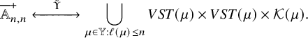
In case
, we have
 $$ \begin{align} \mathrm{wt}(\overline{\pi}) = \mathscr{H}(V) + \mathscr{H}(W) + |\kappa|. \end{align} $$
Proof. One only needs to notice that if
![]() then
then
![]() where the partition
where the partition $\nu $
is equal for both cases. Factoring out information about
$\nu $
is equal for both cases. Factoring out information about $\nu $
, we are left with the desired bijection.
$\nu $
, we are left with the desired bijection.
Clearly, this also induces a bijection
![]() , which we denote by the same notation, where
, which we denote by the same notation, where $\overline {M}\in \overline {\mathbb {M}}^+_{n\times n}$
.
$\overline {M}\in \overline {\mathbb {M}}^+_{n\times n}$
.
8.2 A worked out example
In this subsection, we present an example of bijection $\Upsilon $
defined in equation (8.1). We also take this as an opportunity to review various constructions introduced throughout the text. Let
$\Upsilon $
defined in equation (8.1). We also take this as an opportunity to review various constructions introduced throughout the text. Let
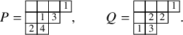
A single iteration of the skew $\mathbf {RSK}$
map yields the pair
$\mathbf {RSK}$
map yields the pair $(P',Q')=\mathbf {RSK}(P,Q)$
as
$(P',Q')=\mathbf {RSK}(P,Q)$
as
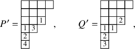
which is $\mathbf {RSK}$
-stable so that vertically strict tableaux
$\mathbf {RSK}$
-stable so that vertically strict tableaux $V,W$
are
$V,W$
are
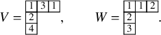
A possible leading map for V is
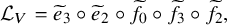 $$ \begin{align} \mathcal{L}_{V} = \widetilde{e}_{3} \circ \widetilde{e}_{2} \circ \widetilde{f}_{0} \circ \widetilde{f}_{3} \circ \widetilde{f}_{2}, \end{align} $$
since

Notice that the $0$
-th Kashiwara operators
$0$
-th Kashiwara operators $\widetilde {f}_{0}$
is, in this particular case, a Demazure arrow. The leading map for W is even simpler and we can take
$\widetilde {f}_{0}$
is, in this particular case, a Demazure arrow. The leading map for W is even simpler and we can take $\mathcal {L}_{W} = \widetilde {e}_{1}$
. Combining
$\mathcal {L}_{W} = \widetilde {e}_{1}$
. Combining $\mathcal {L}_{V}$
and
$\mathcal {L}_{V}$
and $\mathcal {L}_{W}\kern-1pt$
, we produce the leading map for the pair
$\mathcal {L}_{W}\kern-1pt$
, we produce the leading map for the pair $(P,Q)$
,
$(P,Q)$
,
 $$ \begin{align} \mathcal{L}_{P,Q} = \widetilde{E}^{(1)}_3 \circ \widetilde{E}^{(1)}_2 \circ \widetilde{F}^{(1)}_0 \circ \widetilde{F}^{(1)}_3 \circ \widetilde{F}^{(1)}_2 \circ \widetilde{E}^{(2)}_1, \end{align} $$
whose action can be computed as
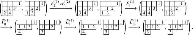
In the right-hand side, we obtained $(T,T)=\mathcal {L}_{P,Q}(P,Q)$
, where T is a leading tableau as it can be checked (more in general this is implied by Proposition 7.21). Using the correspondence of Proposition 7.19, we write T as
$(T,T)=\mathcal {L}_{P,Q}(P,Q)$
, where T is a leading tableau as it can be checked (more in general this is implied by Proposition 7.21). Using the correspondence of Proposition 7.19, we write T as

Therefore, correspondence (8.1), in this case, yields
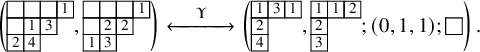
We can finally verify that the relation between empty shape, energies, $\kappa $
and
$\kappa $
and $\nu $
holds, since
$\nu $
holds, since
 $$ \begin{align} \mathscr{H}(V)=1, \qquad \mathscr{H}(W)=0 \end{align} $$
and
 $$ \begin{align} |\rho| = \mathscr{H}(V) + \mathscr{H}(W) + |\kappa| + |\nu| \,\,\, \rightsquigarrow \,\,\, 4 = 1+ 0 + 2 + 1. \end{align} $$
Clearly, reading backward the example we just presented, gives a realization of the inverse map $\Upsilon ^{-1}$
.
$\Upsilon ^{-1}$
.
8.3 Extensions
Arguments and constructions described throughout this paper admit a few natural extensions. We will outline some of these in the next few paragraphs, although, to keep the exposition concise, we will not enter the details of any of the cases we present.
In order to establish Proposition 8.1, we have leveraged properties of the skew $\mathbf {RSK}$
map and of theory of affine crystals. In particular, our skew
$\mathbf {RSK}$
map and of theory of affine crystals. In particular, our skew $\mathbf {RSK}$
map was defined in Section 3 through a sequence of internal row insertions. A natural twist to this story would come from a replacement of row insertions by column insertions as described in [Reference Sagan74, Chapter 3.2]. Call skew
$\mathbf {RSK}$
map was defined in Section 3 through a sequence of internal row insertions. A natural twist to this story would come from a replacement of row insertions by column insertions as described in [Reference Sagan74, Chapter 3.2]. Call skew $\mathbf {RSK}^{\mathrm {col}}$
map the map defined by switching row and column insertions in Proposition 3.1. Then one could define a skew
$\mathbf {RSK}^{\mathrm {col}}$
map the map defined by switching row and column insertions in Proposition 3.1. Then one could define a skew $\mathbf {RSK}^{\mathrm {col}}$
dynamics, which conversely from the skew
$\mathbf {RSK}^{\mathrm {col}}$
dynamics, which conversely from the skew $\mathbf {RSK}$
dynamics, would evolve the shape of tableaux
$\mathbf {RSK}$
dynamics, would evolve the shape of tableaux $(P,Q)$
‘rightward’ rather than ‘downward’. It is natural to expect that repeating arguments developed in this paper one could produce an additional new bijection
$(P,Q)$
‘rightward’ rather than ‘downward’. It is natural to expect that repeating arguments developed in this paper one could produce an additional new bijection
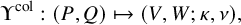 $$ \begin{align} \Upsilon^{\mathrm{col}}:(P,Q) \mapsto (V,W;\kappa,\nu), \end{align} $$
analogous to that of Proposition 8.1. Here, $(P,Q)$
is a pair of semistandard skew tableaux, while this time
$(P,Q)$
is a pair of semistandard skew tableaux, while this time $V,W$
are horizontally weak tableaux (i.e., labels are weakly increasing along rows and no condition is set on columns) of same shape
$V,W$
are horizontally weak tableaux (i.e., labels are weakly increasing along rows and no condition is set on columns) of same shape $\mu $
,
$\mu $
, $\kappa $
is a suitable adaptation of Proposition 7.17 and
$\kappa $
is a suitable adaptation of Proposition 7.17 and $\nu $
is a partition. This would yield a correspondence similar to Shi’s affine Robinson-Schensted correspondence [Reference Shi79] and a comparison between the two constructions would be of much interest.
$\nu $
is a partition. This would yield a correspondence similar to Shi’s affine Robinson-Schensted correspondence [Reference Shi79] and a comparison between the two constructions would be of much interest.
Another natural extension of our theory comes from replacing the skew $\mathbf {RSK}$
map with its dual variant which could be defined following [Reference Sagan and Stanley73, Section 7]. Sagan and Stanley used this idea to put in correspondence pairs
$\mathbf {RSK}$
map with its dual variant which could be defined following [Reference Sagan and Stanley73, Section 7]. Sagan and Stanley used this idea to put in correspondence pairs $(P,Q)$
of semistandard tableaux with conjugate shape with pairs
$(P,Q)$
of semistandard tableaux with conjugate shape with pairs $(\overline {M};\nu )$
consisting of a binary infinite matrix
$(\overline {M};\nu )$
consisting of a binary infinite matrix $\overline {M}$
and a partition
$\overline {M}$
and a partition $\nu $
. Calling skew
$\nu $
. Calling skew $\mathbf {RSK}^{\vee }$
map such dual map, we can define a skew
$\mathbf {RSK}^{\vee }$
map such dual map, we can define a skew $\mathbf {RSK}^\vee $
dynamics in which the P tableau evolves in the ‘downward’ direction, while the Q tableau evolves ‘rightward’ as a result of the fact that their shapes are one the transpose of the other. In this case, it is natural to expect that a reformulation of our arguments would lead to another new bijection
$\mathbf {RSK}^\vee $
dynamics in which the P tableau evolves in the ‘downward’ direction, while the Q tableau evolves ‘rightward’ as a result of the fact that their shapes are one the transpose of the other. In this case, it is natural to expect that a reformulation of our arguments would lead to another new bijection
 $$ \begin{align} \Upsilon^\vee : (P,Q) \mapsto (V,W;\kappa,\nu). \end{align} $$
In this case, $(P,Q)\in SST(\lambda /\rho ,n) \times SST(\lambda ' / \rho ',n)$
, while V and W are, respectively, a vertically strict and a horizontally weak tableaux of conjugate shapes
$(P,Q)\in SST(\lambda /\rho ,n) \times SST(\lambda ' / \rho ',n)$
, while V and W are, respectively, a vertically strict and a horizontally weak tableaux of conjugate shapes $\mu ,\mu '$
,
$\mu ,\mu '$
, $\kappa $
is again a suitable adaptation of the Proposition 7.17 depending on
$\kappa $
is again a suitable adaptation of the Proposition 7.17 depending on $\mu $
and
$\mu $
and $\nu $
is a partition.
$\nu $
is a partition.
We shall consider the two extensions discussed above more precisely in future works.
9 Scattering rules
In this section, we analyse the skew $\mathbf {RSK}$
dynamics from the viewpoint of discrete classical integrable systems, as outlined in Section 1.2. Conservation laws stated in Proposition 6.6 and symmetries of Proposition 5.7 reveal analogies with the renowned BBS introduced in [Reference Takahashi and Satsuma84]; for a review, see [Reference Inoue, Kuniba and Takagi46].
$\mathbf {RSK}$
dynamics from the viewpoint of discrete classical integrable systems, as outlined in Section 1.2. Conservation laws stated in Proposition 6.6 and symmetries of Proposition 5.7 reveal analogies with the renowned BBS introduced in [Reference Takahashi and Satsuma84]; for a review, see [Reference Inoue, Kuniba and Takagi46].
9.1 Setup
In Proposition 4.16, we have defined a pair $(P,Q)$
to be
$(P,Q)$
to be $\mathbf {RSK}$
-stable, if the action of arbitrary many iteration of the skew
$\mathbf {RSK}$
-stable, if the action of arbitrary many iteration of the skew $\mathbf {RSK}$
map on
$\mathbf {RSK}$
map on $(P,Q)$
has the only effect of shifting columns vertically. Analogously, we define a pair
$(P,Q)$
has the only effect of shifting columns vertically. Analogously, we define a pair $(P,Q)$
to be
$(P,Q)$
to be $\mathbf {RSK}^{-1}$
-stable if
$\mathbf {RSK}^{-1}$
-stable if $\mathbf {RSK}^{-t}(P,Q)$
differs from the original pair
$\mathbf {RSK}^{-t}(P,Q)$
differs from the original pair $(P,Q)$
by vertical shifts of the shape, with no changes in the column content. The natural question we address in this section is the following.
$(P,Q)$
by vertical shifts of the shape, with no changes in the column content. The natural question we address in this section is the following.
Question 4. Consider a pair $(P,Q)$
of skew semistandard tableaux, and assume that such pair is
$(P,Q)$
of skew semistandard tableaux, and assume that such pair is $\mathbf {RSK}^{-1}$
-stable. We know that for t large enough
$\mathbf {RSK}^{-1}$
-stable. We know that for t large enough $(\widetilde {P}, \widetilde {Q}) = \mathbf {RSK}^t(P,Q)$
becomes
$(\widetilde {P}, \widetilde {Q}) = \mathbf {RSK}^t(P,Q)$
becomes $\mathbf {RSK}$
-stable. One can think, for instance of pairs of tableaux depicted in the left- and right-hand side of Figure 21. Can we precisely describe
$\mathbf {RSK}$
-stable. One can think, for instance of pairs of tableaux depicted in the left- and right-hand side of Figure 21. Can we precisely describe $(\widetilde {P}, \widetilde {Q})$
purely in terms of
$(\widetilde {P}, \widetilde {Q})$
purely in terms of $(P,Q)$
and t? More specifically, without going through the lengthy procedure of computing the full skew
$(P,Q)$
and t? More specifically, without going through the lengthy procedure of computing the full skew $\mathbf {RSK}$
dynamics:
$\mathbf {RSK}$
dynamics:
-
• Can we predict the content of columns of
$(\widetilde {P}, \widetilde {Q})$
? -
• Can we predict the shape of tableaux
$\widetilde {P}, \widetilde {Q}$
?


A full scattering from an $\mathbf {RSK}^{-1}$
-stable pair on the left to an
$\mathbf {RSK}^{-1}$
-stable pair on the left to an $\mathbf {RSK}$
-stable pair on the right.
$\mathbf {RSK}$
-stable pair on the right.
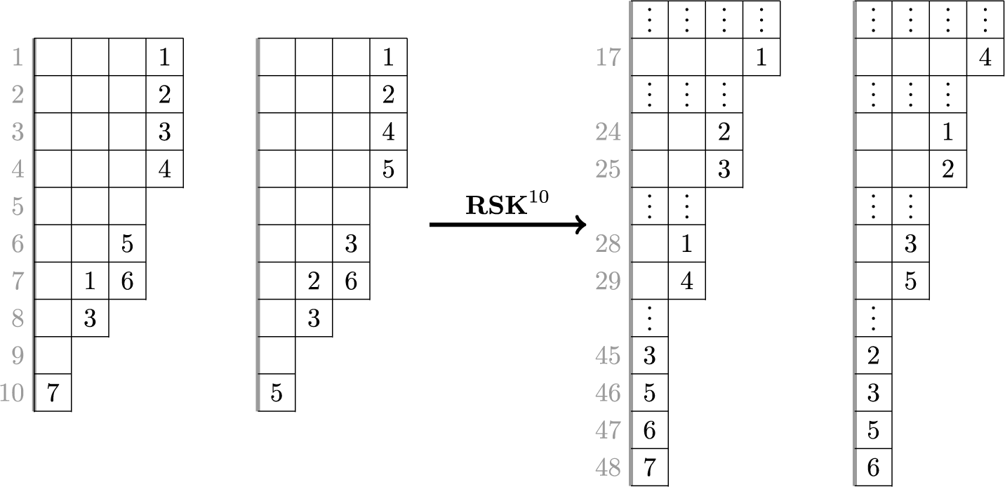
It turns out that Question 4 admits a precise answer, that we present in the two main theorems of this section. In Proposition 9.3, we describe how labeled cells of tableaux $P,Q$
rearrange following the scattering produced by the skew
$P,Q$
rearrange following the scattering produced by the skew $\mathbf {RSK}$
dynamics. Leveraging on linearization techniques of the skew
$\mathbf {RSK}$
dynamics. Leveraging on linearization techniques of the skew $\mathbf {RSK}$
map elaborated in Section 7, the task of describing the shape of
$\mathbf {RSK}$
map elaborated in Section 7, the task of describing the shape of $(\widetilde {P},\widetilde {Q})$
becomes then a simple exercise. We present it in Proposition 9.7 in Section 9.3.
$(\widetilde {P},\widetilde {Q})$
becomes then a simple exercise. We present it in Proposition 9.7 in Section 9.3.
9.2 Scattering in the skew
$\mathbf {RSK}$
dynamics

Fix $P,Q\in SST(\lambda / \rho ,n)$
, and consider the skew
$P,Q\in SST(\lambda / \rho ,n)$
, and consider the skew $\mathbf {RSK}$
dynamics
$\mathbf {RSK}$
dynamics $(P_t,Q_t)$
with initial data
$(P_t,Q_t)$
with initial data $(P,Q)$
. For any t, define
$(P,Q)$
. For any t, define $v^{(t)}=v^{(t)}_1 \otimes \cdots \otimes v^{(t)}_{\lambda _1}$
to be the element of the crystal
$v^{(t)}=v^{(t)}_1 \otimes \cdots \otimes v^{(t)}_{\lambda _1}$
to be the element of the crystal $B^{\varkappa (t)}$
formed by the tensor product of columns of
$B^{\varkappa (t)}$
formed by the tensor product of columns of $P_t$
. Analogously, define
$P_t$
. Analogously, define $u^{(t)}=u^{(t)}_1 \otimes \cdots \otimes u^{(t)}_{\lambda _1}$
from columns of
$u^{(t)}=u^{(t)}_1 \otimes \cdots \otimes u^{(t)}_{\lambda _1}$
from columns of $Q_t$
. Composition
$Q_t$
. Composition $\varkappa (t)$
records then the number of labeled elements at each column of
$\varkappa (t)$
records then the number of labeled elements at each column of $P_t,Q_t$
. We have seen in Section 6 that, when t becomes large,
$P_t,Q_t$
. We have seen in Section 6 that, when t becomes large, $\varkappa (t) \xrightarrow [t\to \infty ]{} \mu '$
, where
$\varkappa (t) \xrightarrow [t\to \infty ]{} \mu '$
, where $\mu $
is the Greene invariant of
$\mu $
is the Greene invariant of $\overline {\pi }$
related to
$\overline {\pi }$
related to $(P,Q)$
by the Sagan–Stanley correspondence
$(P,Q)$
by the Sagan–Stanley correspondence $(P,Q) \xrightarrow []{\mathbf {SS} \,} \overline {\pi }$
. Analogously, we can consider
$(P,Q) \xrightarrow []{\mathbf {SS} \,} \overline {\pi }$
. Analogously, we can consider $\varkappa (t)$
for
$\varkappa (t)$
for $t\to -\infty $
. In the following theorem, we denote with
$t\to -\infty $
. In the following theorem, we denote with $\overleftarrow {\eta }=(\eta _N,\dots ,\eta _1)$
the reverse ordering of a partition
$\overleftarrow {\eta }=(\eta _N,\dots ,\eta _1)$
the reverse ordering of a partition $\eta = (\eta _1,\dots ,\eta _N)$
.
$\eta = (\eta _1,\dots ,\eta _N)$
.
Theorem 9.1. In the notation introduced above, we have $\varkappa (-t) = \overleftarrow {\mu }'$
eventually for t large enough.
$\varkappa (-t) = \overleftarrow {\mu }'$
eventually for t large enough.
Proof. In Proposition 6.6, we have related the asymptotic increment $\varkappa (t)$
for
$\varkappa (t)$
for $t \gg 0$
with conserved quantities of the Viennot map
$t \gg 0$
with conserved quantities of the Viennot map $\mathbf {V}$
, yielding the equality
$\mathbf {V}$
, yielding the equality $\varkappa (t)=\mu '$
. Analogously, we can relate backward asymptotic increments
$\varkappa (t)=\mu '$
. Analogously, we can relate backward asymptotic increments $\varkappa (-t)$
for
$\varkappa (-t)$
for $t \gg 0$
with conserved quantities of the inverse Viennot map
$t \gg 0$
with conserved quantities of the inverse Viennot map $\mathbf {V}^{-1}$
, which are the same as
$\mathbf {V}^{-1}$
, which are the same as $\mathbf {V}$
. Through such argument one can easily complete the proof.
$\mathbf {V}$
. Through such argument one can easily complete the proof.
Remark 9.2. In view of Proposition 9.1, columns of tableaux in the skew $\mathbf {RSK}$
dynamics may be seen as solitons. Thanks to conservation laws, they survive after collisions with others and eventually propagate at their own characteristic speeds, similarly to the ones in BBS. In the case of the BBS, conservation of solitons can be proven in several different ways. These include commutation of transfer matrices [Reference Fukuda, Okado and Yamada30] or bijection with rigged configuration through the Kerov–Kirillov–Reshetikhin (KKR) correspondence [Reference Kuniba, Okado, Sakamoto, Takagi and Yamada56]. Similarities between the BBS and the skew
$\mathbf {RSK}$
dynamics may be seen as solitons. Thanks to conservation laws, they survive after collisions with others and eventually propagate at their own characteristic speeds, similarly to the ones in BBS. In the case of the BBS, conservation of solitons can be proven in several different ways. These include commutation of transfer matrices [Reference Fukuda, Okado and Yamada30] or bijection with rigged configuration through the Kerov–Kirillov–Reshetikhin (KKR) correspondence [Reference Kuniba, Okado, Sakamoto, Takagi and Yamada56]. Similarities between the BBS and the skew $\mathbf {RSK}$
dynamics provided by Propositions 9.1, 9.3 and 9.7 suggest that the framework developed in this paper might provide an alternative, more combinatorial, route to study the BBS. It would be interesting to understand relations between our results and KKR correspondence or even to understand extension of such correspondence in types other than
$\mathbf {RSK}$
dynamics provided by Propositions 9.1, 9.3 and 9.7 suggest that the framework developed in this paper might provide an alternative, more combinatorial, route to study the BBS. It would be interesting to understand relations between our results and KKR correspondence or even to understand extension of such correspondence in types other than $A^{(1)}_{n-1}$
. We plan to pursue these directions in future publications.
$A^{(1)}_{n-1}$
. We plan to pursue these directions in future publications.
Carrying on with the notation introduced at the beginning of the present subsection, we see elements $v^{(t)},u^{(t)}\in B^{\varkappa (t)}$
become, for large t equivalent to the asymptotic vertically strict tableaux of Proposition 4.17. Analogously,
$v^{(t)},u^{(t)}\in B^{\varkappa (t)}$
become, for large t equivalent to the asymptotic vertically strict tableaux of Proposition 4.17. Analogously, $v^{(-t)},u^{(-t)}$
, for large t, eventually stabilize and we define the limits
$v^{(-t)},u^{(-t)}$
, for large t, eventually stabilize and we define the limits
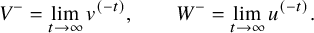 $$ \begin{align} V^-=\lim_{t \to \infty} v^{(-t)}, \qquad W^-=\lim_{t \to \infty} u^{(-t)}. \end{align} $$
By Proposition 9.1 we have $V^-, W^- \in B^{\overleftarrow {\mu }'}$
and we define the backward projection
$V^-, W^- \in B^{\overleftarrow {\mu }'}$
and we define the backward projection
 $$ \begin{align} \Phi^-:(P,Q) \mapsto (V^-, W^-), \end{align} $$
as the negative time counterpart of $\Phi $
given in equation (4.21).
$\Phi $
given in equation (4.21).
The relation between the backward and forward asymptotic states $(V^-,W^-)$
and
$(V^-,W^-)$
and $(V,W)$
gives the scattering rules of solitons in the skew
$(V,W)$
gives the scattering rules of solitons in the skew $\mathbf {RSK}$
dynamics. A typical feature of integrable systems is that effects of multibody scattering are fully determined by the knowledge of the two-body scattering. In the case of BBSs, two body scattering is given by the combinatorial
$\mathbf {RSK}$
dynamics. A typical feature of integrable systems is that effects of multibody scattering are fully determined by the knowledge of the two-body scattering. In the case of BBSs, two body scattering is given by the combinatorial $\mathscr {R}$
-matrix. The following theorem claims that the scattering rules relating
$\mathscr {R}$
-matrix. The following theorem claims that the scattering rules relating $(V^-,W^-)$
and
$(V^-,W^-)$
and $(V,W)$
in our skew
$(V,W)$
in our skew $\mathbf {RSK}$
dynamics are also described by consecutive applications of the same combinatorial
$\mathbf {RSK}$
dynamics are also described by consecutive applications of the same combinatorial $\mathscr {R}$
matrices corresponding to the change of orders of solitons. In order to give a precise statement, we define, following Proposition 7.3, the unique isomorphism of crystal graphs
$\mathscr {R}$
matrices corresponding to the change of orders of solitons. In order to give a precise statement, we define, following Proposition 7.3, the unique isomorphism of crystal graphs $B^\mu \to B^{\overleftarrow {\mu }'}$
. It is expressed, naming
$B^\mu \to B^{\overleftarrow {\mu }'}$
. It is expressed, naming $\delta (N)$
the permutation
$\delta (N)$
the permutation $(N \,\, \, N-1 \,\, \, \cdots \,\,\, 1)$
, as
$(N \,\, \, N-1 \,\, \, \cdots \,\,\, 1)$
, as
For an example of the action of $\mathscr {R}_{\delta (\mu _1)}$
, see equation (9.8) below.
$\mathscr {R}_{\delta (\mu _1)}$
, see equation (9.8) below.
Theorem 9.3. Let $(P,Q)$
be a pair of tableaux, call
$(P,Q)$
be a pair of tableaux, call $\mu $
the respective Greene invariant and consider the projections
$\mu $
the respective Greene invariant and consider the projections
 $$ \begin{align} \Phi(P,Q) = (V, W), \qquad \Phi^-(P,Q) = (V^-, W^-). \end{align} $$
Then the map $\Psi :(V,W) \to (V^-, W^-)$
is well defined, does not depend on the choice of
$\Psi :(V,W) \to (V^-, W^-)$
is well defined, does not depend on the choice of $(P,Q)$
and it is given by
$(P,Q)$
and it is given by
 $$ \begin{align} V^-= \mathscr{R}_{\delta(\mu_1)} (V), \qquad W^-= \mathscr{R}_{\delta(\mu_1)} (W). \end{align} $$
Proof. Define $\psi =\mathscr {R}_{\delta (\mu _1)}$
. We will only show that
$\psi =\mathscr {R}_{\delta (\mu _1)}$
. We will only show that $V^- = \psi (V)$
since the same relation for
$V^- = \psi (V)$
since the same relation for $V,W^-$
can be proven in analogous fashion. This defines maps
$V,W^-$
can be proven in analogous fashion. This defines maps
 $$ \begin{align} \phi^+:(P,Q) \mapsto V \qquad \text{and} \qquad \phi^-:(P,Q) \mapsto V^-. \end{align} $$
The proof Proposition 9.3 reduces to characterizing the map $V^- \mapsto V$
and to prove that it is given by
$V^- \mapsto V$
and to prove that it is given by $\psi ^{-1}$
. Notice that in principle such map could be not well defined since there might exist pairs
$\psi ^{-1}$
. Notice that in principle such map could be not well defined since there might exist pairs $(P,Q),(P',Q')$
such that, for instance,
$(P,Q),(P',Q')$
such that, for instance, $\phi ^-(P,Q)=\phi ^-(P',Q')$
, but
$\phi ^-(P,Q)=\phi ^-(P',Q')$
, but $\phi ^+(P,Q) \neq \phi ^+(P',Q')$
. We show that this is indeed not the case.
$\phi ^+(P,Q) \neq \phi ^+(P',Q')$
. We show that this is indeed not the case.
Fix an element $V^- \in B^{\overleftarrow {\mu }'}$
, and consider a pair
$V^- \in B^{\overleftarrow {\mu }'}$
, and consider a pair $(P,Q)$
such that
$(P,Q)$
such that $\phi ^-(P,Q) = V^-$
. Notice first that if
$\phi ^-(P,Q) = V^-$
. Notice first that if $V^-$
is the leading vector
$V^-$
is the leading vector $V^-=(\overleftarrow {\mu }')^{\mathrm {lv}}$
, then necessarily
$V^-=(\overleftarrow {\mu }')^{\mathrm {lv}}$
, then necessarily $\gamma (P)=\mu $
and
$\gamma (P)=\mu $
and $V=(\mu ')^{\mathrm {lv}}$
. For more general
$V=(\mu ')^{\mathrm {lv}}$
. For more general $V^-$
, we can always connect it to the leading vector
$V^-$
, we can always connect it to the leading vector $(\overleftarrow {\mu }')^{\mathrm {lv}}$
through a leading map
$(\overleftarrow {\mu }')^{\mathrm {lv}}$
through a leading map $\mathcal {L}_{V^-}$
, as in Proposition 7.8. The
$\mathcal {L}_{V^-}$
, as in Proposition 7.8. The $\Phi $
-pullback of
$\Phi $
-pullback of $\mathcal {L}_{V^-}$
defines a map on pairs of tableaux
$\mathcal {L}_{V^-}$
defines a map on pairs of tableaux $\mathcal {L}_{V^-}:(P,Q) \to (P',Q')$
, which commutes with the skew
$\mathcal {L}_{V^-}:(P,Q) \to (P',Q')$
, which commutes with the skew $\mathbf {RSK}$
map and hence with projection
$\mathbf {RSK}$
map and hence with projection $\Phi $
. This shows that fixed
$\Phi $
. This shows that fixed $V^-$
, we always have
$V^-$
, we always have
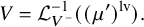 $$ \begin{align} V=\mathcal{L}_{V^-}^{-1}((\mu')^{\mathrm{lv}}). \end{align} $$
Comparing equation (9.7) with result of Proposition 5.5, we can conclude that map $V\mapsto V^-$
exists and it is the unique isomorphism of crystals
$V\mapsto V^-$
exists and it is the unique isomorphism of crystals $B^{\mu '}, B^{\overleftarrow {\mu }'}$
and by Proposition 7.3 we have
$B^{\mu '}, B^{\overleftarrow {\mu }'}$
and by Proposition 7.3 we have $V=\psi ^{-1}(V^-)$
. Notice that this is independently of the choice of
$V=\psi ^{-1}(V^-)$
. Notice that this is independently of the choice of $(P,Q)$
, as long as
$(P,Q)$
, as long as $\phi ^-(P,Q)=V^-$
.
$\phi ^-(P,Q)=V^-$
.
Example 9.4. We can verify the statement of Proposition 9.3 in the example reported in Figure 21. The transformation $V \mapsto V^-$
step by step, reads
$V \mapsto V^-$
step by step, reads
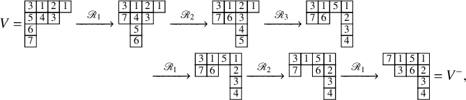
where we have suppressed symbol $\otimes $
between different columns.
$\otimes $
between different columns.
Remark 9.5. In [Reference Chmutov, Frieden, Kim, Lewis and Yudovina19], authors described an analogous phenomenon as that of Proposition 9.3 in the context of affine matrix ball construction. In that paper, the operation called affine evacuation $V\mapsto \mathrm {evac}(V)$
corresponds to transforming element
$V\mapsto \mathrm {evac}(V)$
corresponds to transforming element $V^-$
in a vertically strict tableaux of shape equal to V, rotating
$V^-$
in a vertically strict tableaux of shape equal to V, rotating $V^-$
by
$V^-$
by $180^\circ $
and replacing each entry i by
$180^\circ $
and replacing each entry i by $n-i+1$
.
$n-i+1$
.
Remark 9.6. Note that similarities between the exchange of degrees of freedom for solitons in the BBS and vertically strict tableaux in the skew $\mathbf {RSK}$
dynamics do not imply that all properties of the skew
$\mathbf {RSK}$
dynamics do not imply that all properties of the skew $\mathbf {RSK}$
dynamics can be studied by standard techniques of the BBS. For instance, it is not clear if one could express the skew
$\mathbf {RSK}$
dynamics can be studied by standard techniques of the BBS. For instance, it is not clear if one could express the skew $\mathbf {RSK}$
map as a transfer matrix, that is, as a product of local R-matrices. To understand fully relations between the two models, more elaborated considerations are needed.
$\mathbf {RSK}$
map as a transfer matrix, that is, as a product of local R-matrices. To understand fully relations between the two models, more elaborated considerations are needed.
9.3 Phase shift
Leveraging on results discussed in Section 7.5, here we describe the phase shift in the scattering between columns of different length in the skew $\mathbf {RSK}$
dynamics. As we explained, each soliton has its own speed, not changing after collisions. But its phase, which determines the position of the linear trajectory of a soliton, may shift during a collision with another one. This is the phase shift. It is an important notion in soliton theory because together with the description of exchanges of degrees of freedom it completely characterizes the whole scattering process of solitons.
$\mathbf {RSK}$
dynamics. As we explained, each soliton has its own speed, not changing after collisions. But its phase, which determines the position of the linear trajectory of a soliton, may shift during a collision with another one. This is the phase shift. It is an important notion in soliton theory because together with the description of exchanges of degrees of freedom it completely characterizes the whole scattering process of solitons.
The phase shift in the skew $\mathbf {RSK}$
dynamics may be well explained by the example in Figure 21. There, we see that, in the left-hand side the column hosting four labeled cells, which we call 4-soliton, ‘starts’ at the first row. After 10 iterations of the skew
$\mathbf {RSK}$
dynamics may be well explained by the example in Figure 21. There, we see that, in the left-hand side the column hosting four labeled cells, which we call 4-soliton, ‘starts’ at the first row. After 10 iterations of the skew $\mathbf {RSK}$
map, when all collisions are completed, we see that, in the tableaux on the right-hand side, the 4-soliton in the first column occupies rows 45 to 48. This means that interactions with other columns have accelerated the motion of the 4-soliton, which otherwise would have traveled only
$\mathbf {RSK}$
map, when all collisions are completed, we see that, in the tableaux on the right-hand side, the 4-soliton in the first column occupies rows 45 to 48. This means that interactions with other columns have accelerated the motion of the 4-soliton, which otherwise would have traveled only $4\times 10 = 40$
cells. In this case, the phase shift was equal to 4. The same phenomenon can be observed also tracking locations of other columns of the tableaux.
$4\times 10 = 40$
cells. In this case, the phase shift was equal to 4. The same phenomenon can be observed also tracking locations of other columns of the tableaux.
The next theorem gives a precise description of phase shifts in the skew $\mathbf {RSK}$
dynamics and gives a a full answer to the second bullet of Question 4.
$\mathbf {RSK}$
dynamics and gives a a full answer to the second bullet of Question 4.
Theorem 9.7. Let $(P,Q)$
be an
$(P,Q)$
be an $\mathbf {RSK}^{-1}$
-stable pair of skew tableaux of shape
$\mathbf {RSK}^{-1}$
-stable pair of skew tableaux of shape $\lambda /\rho $
, and assume
$\lambda /\rho $
, and assume $\ker (P,Q)=\varnothing $
. Denote the Greene invariant of
$\ker (P,Q)=\varnothing $
. Denote the Greene invariant of $(P,Q)$
by
$(P,Q)$
by $\mu $
and define its rectangular decomposition by indices
$\mu $
and define its rectangular decomposition by indices $0=R_0,R_1,\dots ,R_N=\mu _1$
and
$0=R_0,R_1,\dots ,R_N=\mu _1$
and $r_i$
as discussed around equation (2.9). Moreover, set
$r_i$
as discussed around equation (2.9). Moreover, set $\widetilde {R}_i = R_N - R_{i+1}$
. Let t be large enough so that
$\widetilde {R}_i = R_N - R_{i+1}$
. Let t be large enough so that $(\widetilde {P},\widetilde {Q})=\mathbf {RSK}^t (P,Q)$
is
$(\widetilde {P},\widetilde {Q})=\mathbf {RSK}^t (P,Q)$
is $\mathbf {RSK}$
-stable and denote by
$\mathbf {RSK}$
-stable and denote by $\widetilde {\lambda } / \widetilde {\rho }$
the shape of
$\widetilde {\lambda } / \widetilde {\rho }$
the shape of $(\widetilde {P},\widetilde {Q})$
. Then the phase shift of the j-th column of length
$(\widetilde {P},\widetilde {Q})$
. Then the phase shift of the j-th column of length $\mu _{R_{i+1}}^{\prime }$
is given by
$\mu _{R_{i+1}}^{\prime }$
is given by
 $$ \begin{align} \widetilde{\rho}_{R_i + j}^{\, \prime} - \rho_{\widetilde{R}_i + j}^{\prime} - t \times \mu_{R_{i+1}}^{\prime} = \mathscr{H}_{R_i + j}(V)+\mathscr{H}_{R_i + j}(W) - \mathscr{H}_{\widetilde{R}_i + j}(V^-) - \mathscr{H}_{\widetilde{R}_i + j}(W^-), \end{align} $$
for all $i=0,\dots ,N-1, j=1,\dots ,r_{i+1}$
and where
$i=0,\dots ,N-1, j=1,\dots ,r_{i+1}$
and where $(V^-,W^-) = \Phi ^-(P,Q)$
, while
$(V^-,W^-) = \Phi ^-(P,Q)$
, while $(V, W) = \Phi (P,Q)$
.
$(V, W) = \Phi (P,Q)$
.
Proof. Let $\mathcal {L}_{P,Q}$
be the leading map of the pair
$\mathcal {L}_{P,Q}$
be the leading map of the pair $(P,Q)$
, and let
$(P,Q)$
, and let $T=T(\mu ,\kappa ;\varnothing )$
be the leading tableau such that
$T=T(\mu ,\kappa ;\varnothing )$
be the leading tableau such that $(T,T)=\mathcal {L}_{P,Q}(P,Q)$
. In order to prove our claim, we make use of commutation relation
$(T,T)=\mathcal {L}_{P,Q}(P,Q)$
. In order to prove our claim, we make use of commutation relation
 $$ \begin{align} (\widetilde{P},\widetilde{Q}) = \mathcal{L}_{P,Q}^{-1} \circ \mathbf{RSK}^{t} \circ \mathcal{L}_{P,Q} (P,Q), \end{align} $$
which follows from Proposition 5.7. Since $(P,Q)$
is
$(P,Q)$
is $\mathbf {RSK}^{-1}$
-stable so is
$\mathbf {RSK}^{-1}$
-stable so is $(T,T)$
and hence
$(T,T)$
and hence $\kappa =(\kappa ^{(1)},\dots , \kappa ^{(N)})$
is of the form
$\kappa =(\kappa ^{(1)},\dots , \kappa ^{(N)})$
is of the form
 $$ \begin{align} \kappa^{(N)}_1 \ge \cdots \ge \kappa^{(N)}_{r_N}> \kappa^{(N-1)}_1 \ge \cdots \kappa^{(N-1)}_{r_{N-1}}> \cdots \ge \kappa^{(1)}_1 > \cdots > \kappa^{(1)}_{r_1}. \end{align} $$
From Proposition 7.19, the empty shape of T is $(\kappa ^+)'$
and by Proposition 5.12 we have
$(\kappa ^+)'$
and by Proposition 5.12 we have
 $$ \begin{align} \rho_i^{\prime} = \kappa^+_i + \mathscr{H}_i(V^-) + \mathscr{H}_i(W^-), \end{align} $$
where $\kappa ^+$
is explicitly determined by equation (9.11). Applying t times the skew
$\kappa ^+$
is explicitly determined by equation (9.11). Applying t times the skew $\mathbf {RSK}$
map to pair
$\mathbf {RSK}$
map to pair $(T,T)$
, we obtain, by Proposition 7.22,
$(T,T)$
, we obtain, by Proposition 7.22,
 $$ \begin{align} (\widetilde{T},\widetilde{T}) = \mathbf{RSK}^t(T,T), \qquad \text{where} \qquad \widetilde{T}=T(\mu,\widetilde{\kappa};\varnothing), \qquad \widetilde{\kappa}=\kappa + t \times \mu'. \end{align} $$
When t is large, as in the hypothesis of the theorem, we have that $\widetilde {\kappa }$
is itself a partition and hence the empty shape of
$\widetilde {\kappa }$
is itself a partition and hence the empty shape of $\widetilde {T}$
is given by
$\widetilde {T}$
is given by $\widetilde {\kappa }'$
. The action of the map
$\widetilde {\kappa }'$
. The action of the map $\mathcal {L}^{-1}_{P,Q}$
on
$\mathcal {L}^{-1}_{P,Q}$
on $(\widetilde {T}, \widetilde {T})$
has the effect of growing the empty shape as prescribed by Proposition 5.12, implying
$(\widetilde {T}, \widetilde {T})$
has the effect of growing the empty shape as prescribed by Proposition 5.12, implying
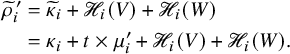 $$ \begin{align} \begin{aligned}\widetilde{\rho}^{\, \prime}_i &= \widetilde{\kappa}_i + \mathscr{H}_i(V) + \mathscr{H}_i(W) \\&=\kappa_i + t \times \mu_i^{\prime} + \mathscr{H}_i(V) + \mathscr{H}_i(W).\end{aligned} \end{align} $$
Expressing the term $\kappa _i$
in terms of
$\kappa _i$
in terms of $\rho '$
and of local energies of elements
$\rho '$
and of local energies of elements $V^-,W^-$
yields equation (9.9).
$V^-,W^-$
yields equation (9.9).
Example 9.8. We can confirm the validity of Proposition 9.7 computing equation (9.9) for tableaux presented in Figure 21. For that case, in the notation of Proposition 9.7, we have
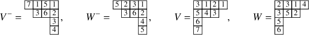
so that we can compute the local energies
 $$ \begin{align} (\mathscr{H}_i(V^-))_{i=1,\dots,4} = (2,2,2,0), \qquad (\mathscr{H}_i(W^-))_{i=1,\dots,4} = (1,1,1,0), \end{align} $$
 $$ \begin{align} (\mathscr{H}_i(V))_{i=1,\dots,4} = (3,2,1,0), \qquad (\mathscr{H}_i(W))_{i=1,\dots,4} = (1,2,0,0). \end{align} $$
Then, equations (9.9) reduce to
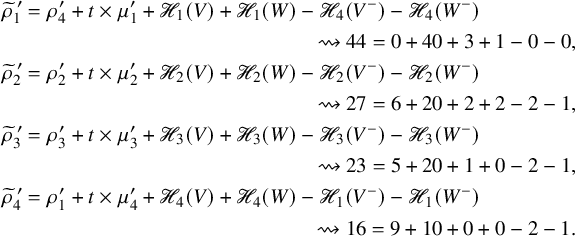 $$ \begin{gather*} \widetilde{\rho}_{1}^{\, \prime} = \rho_{4}^{\prime} + t \times \mu_{1}^{\prime} +\mathscr{H}_{1}(V)+\mathscr{H}_{1}(W) - \mathscr{H}_{4}(V^-) - \mathscr{H}_{4}(W^-) \\ \hspace{7cm} \rightsquigarrow 44 = 0 + 40 + 3 + 1 - 0 - 0 , \\ \widetilde{\rho}_{2}^{\, \prime} = \rho_{2}^{\prime} + t \times \mu_{2}^{\prime} +\mathscr{H}_{2}(V)+\mathscr{H}_{2}(W) - \mathscr{H}_{2}(V^-) - \mathscr{H}_{2}(W^-) \\ \hspace{7cm} \rightsquigarrow 27 = 6 + 20 + 2 + 2 - 2 - 1 , \\ \widetilde{\rho}_{3}^{\, \prime} = \rho_{3}^{\prime} + t \times \mu_{3}^{\prime} +\mathscr{H}_{3}(V)+\mathscr{H}_{3}(W) - \mathscr{H}_{3}(V^-) - \mathscr{H}_{3}(W^-) \\ \hspace{7cm} \rightsquigarrow 23 = 5 + 20 + 1 + 0 - 2 - 1 , \\ \widetilde{\rho}_{4}^{\, \prime} = \rho_{1}^{\prime} + t \times \mu_{4}^{\prime} + \mathscr{H}_{4}(V)+\mathscr{H}_{4}(W) - \mathscr{H}_{1}(V^-) - \mathscr{H}_{1}(W^-) \\ \hspace{7cm} \rightsquigarrow 16 = 9 + 10 + 0 + 0 - 2 - 1. \end{gather*} $$
Notice the nontrivial pairing in the previous equalities between columns of $\widetilde {\rho }$
and
$\widetilde {\rho }$
and $\rho $
. In particular, indices are not simply reversed, but they are given by numbers
$\rho $
. In particular, indices are not simply reversed, but they are given by numbers $R_i,\widetilde {R}_i$
as in Proposition 9.7.
$R_i,\widetilde {R}_i$
as in Proposition 9.7.
Remark 9.9. Formulas similar to those in Proposition 9.7 for the phase shift have been found for the BBS [Reference Fukuda, Okado and Yamada30]. In particular, when in the skew $\mathbf {RSK}$
dynamics we consider initial conditions with
$\mathbf {RSK}$
dynamics we consider initial conditions with $P=Q$
, which forces
$P=Q$
, which forces $P_t=Q_t$
for all t, then the phase shift of solitons in multispecies BBS is exactly the same as the one resulting from equation (9.9). Under these assumptions on the initial conditions, the skew
$P_t=Q_t$
for all t, then the phase shift of solitons in multispecies BBS is exactly the same as the one resulting from equation (9.9). Under these assumptions on the initial conditions, the skew $\mathbf {RSK}$
dynamics and the BBS become very similar models and they both possess
$\mathbf {RSK}$
dynamics and the BBS become very similar models and they both possess $\widehat {\mathfrak {sl}}_n$
symmetry. On the other hand, for general initial data
$\widehat {\mathfrak {sl}}_n$
symmetry. On the other hand, for general initial data $P,Q$
the skew
$P,Q$
the skew $\mathbf {RSK}$
dynamics possesses a larger set of symmetries (i.e.,
$\mathbf {RSK}$
dynamics possesses a larger set of symmetries (i.e., $\widehat {\mathfrak {sl}}_n \times \widehat {\mathfrak {sl}}_n$
) and they are no longer equivalent. We shall examine precisely analogies between the BBS and skew
$\widehat {\mathfrak {sl}}_n \times \widehat {\mathfrak {sl}}_n$
) and they are no longer equivalent. We shall examine precisely analogies between the BBS and skew $\mathbf {RSK}$
dynamics in a future work.
$\mathbf {RSK}$
dynamics in a future work.
10 Summation identities and bijective proofs
We explore the consequences of bijection $\Upsilon $
proving a number of summation identities for q-Whittaker polynomials. These are known Cauchy and Littlewood identities, presented in Section 10.1 along with new identities between summations of q-Whittaker and skew Schur polynomials, which are presented in Section 10.2.
$\Upsilon $
proving a number of summation identities for q-Whittaker polynomials. These are known Cauchy and Littlewood identities, presented in Section 10.1 along with new identities between summations of q-Whittaker and skew Schur polynomials, which are presented in Section 10.2.
10.1 Summation identities for q-Whittaker polynomials
The bijection discussed in Section 8.1 reveals a number of combinatorial properties of q-Whittaker polynomials $\mathscr {P}_{\mu }(x;q)$
, that are Macdonald polynomials
$\mathscr {P}_{\mu }(x;q)$
, that are Macdonald polynomials $\mathscr {P}_{\mu }(x;q,t)$
specialized at
$\mathscr {P}_{\mu }(x;q,t)$
specialized at $t=0$
[Reference Macdonald62, Chapter VI]. These have several different representations. For our purposes, the most useful one is given by the combinatorial formula reported in the next proposition as a sum over vertically strict tableaux [Reference Schilling and Tingley77, Corollary 9.5]; see also [Reference Nakayashiki and Yamada65]. The meaning of such expression is that q-Whittaker polynomials are characters of certain Demazure modules of
$t=0$
[Reference Macdonald62, Chapter VI]. These have several different representations. For our purposes, the most useful one is given by the combinatorial formula reported in the next proposition as a sum over vertically strict tableaux [Reference Schilling and Tingley77, Corollary 9.5]; see also [Reference Nakayashiki and Yamada65]. The meaning of such expression is that q-Whittaker polynomials are characters of certain Demazure modules of $\widehat {\mathfrak {sl}}_n$
[Reference Sanderson75], whose grading is given by the intrinsic energy function [Reference Schilling and Tingley77].
$\widehat {\mathfrak {sl}}_n$
[Reference Sanderson75], whose grading is given by the intrinsic energy function [Reference Schilling and Tingley77].
Proposition 10.1. For all partitions $\mu $
, we have
$\mu $
, we have
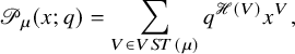 $$ \begin{align} \mathscr{P}_{\mu}(x;q) = \sum_{V\in VST(\mu)} q^{\mathscr{H}(V)} x^V, \end{align} $$
where $x^V=x_1^{m_1(V)} x_2^{m_2(V)} \cdots $
and
$x^V=x_1^{m_1(V)} x_2^{m_2(V)} \cdots $
and $m_i(V)$
counts the number of i-cells in V.
$m_i(V)$
counts the number of i-cells in V.
When $q=0$
, equation (10.1) reduces to the well-known combinatorial formula for the Schur polynomial reported below in equation (10.35), where one should set
$q=0$
, equation (10.1) reduces to the well-known combinatorial formula for the Schur polynomial reported below in equation (10.35), where one should set $\rho =\varnothing $
.
$\rho =\varnothing $
.
Symmetric polynomials $\mathscr {P}_{\mu }$
enjoy Cauchy identities, as reported in [Reference Macdonald62], for the case of general Macdonald polynomials. Leveraging the correspondence reported in Proposition 8.2, here we present a bijective proof. We use the notion of q-Pochhammer symbol
$\mathscr {P}_{\mu }$
enjoy Cauchy identities, as reported in [Reference Macdonald62], for the case of general Macdonald polynomials. Leveraging the correspondence reported in Proposition 8.2, here we present a bijective proof. We use the notion of q-Pochhammer symbol
 $$ \begin{align} (z;q)_k = \prod_{i=0}^{k-1} (1-q^i z) \qquad \text{and} \qquad (z;q)_{\infty} = \prod_{i=0}^\infty (1-q^i z), \end{align} $$
where the second expression holds for $|q|<1$
.
$|q|<1$
.
Theorem 10.2. Fix $|q|<1$
. Consider variables
$|q|<1$
. Consider variables $x=(x_1,\dots ,x_n)$
and
$x=(x_1,\dots ,x_n)$
and $y=(y_1,\dots ,y_n)$
with
$y=(y_1,\dots ,y_n)$
with $|x_i y_j|<1$
for all
$|x_i y_j|<1$
for all $i,j$
. Then
$i,j$
. Then
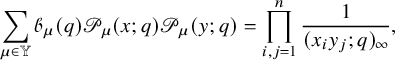
where
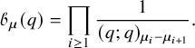
Proof. We start by noticing that
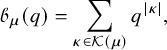
which follows from the summation identity
 $$ \begin{align} \sum_{\substack{\nu \in \mathbb{Y} \\ \nu_1 \le N}} q^{|\nu|} = \frac{1}{(q;q)_N}. \end{align} $$
Then, using equation (10.1) and Proposition 8.2 we deduce the following equalities
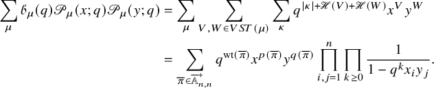
Taking summations over the set of symmetric weighted biwords $\overline {\pi } = \overline {\pi }^{-1}$
yields identities involving single polynomials
$\overline {\pi } = \overline {\pi }^{-1}$
yields identities involving single polynomials $\mathscr {P}_{\mu }$
. To state our result, we define
$\mathscr {P}_{\mu }$
. To state our result, we define
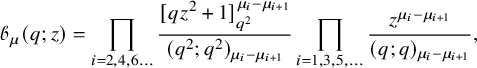
where
 $$ \begin{align} [A+B]_p^k = \sum_{j=0}^k A^j B^{k-j} \binom{k}{j}_{\hspace{-2pt} p} \end{align} $$
and
 $$ \begin{align} \binom{k}{j}_{\hspace{-2pt} p} = \frac{(p;p)_k}{(p;p)_j (p;p)_{k-j}} \end{align} $$
is the Gaussian binomial coefficient. In literature, the function $h_n(x;p) = [x+1]_p^n$
is commonly known as Rogers–Szegö polynomial [Reference Andrews3].
$h_n(x;p) = [x+1]_p^n$
is commonly known as Rogers–Szegö polynomial [Reference Andrews3].
Theorem 10.3. Fix $|q|<1$
. Consider variables z and
$|q|<1$
. Consider variables z and $x=(x_1,\dots ,x_n)$
with
$x=(x_1,\dots ,x_n)$
with $|z x_i|<1$
for all
$|z x_i|<1$
for all $i,j$
. Then we have
$i,j$
. Then we have
Notice that setting $z=0$
in equation (10.11) and using the convention
$z=0$
in equation (10.11) and using the convention $0^0=1$
, since
$0^0=1$
, since
![]() , we obtain the Littlewood identity for q-Whittaker polynomials
, we obtain the Littlewood identity for q-Whittaker polynomials
which becomes (i) of Example 4 in Chapter VI,7 of [Reference Macdonald62], after rescaling $q^2 \to q$
. On the other hand, taking
$q^2 \to q$
. On the other hand, taking $z=1$
, we observe that
$z=1$
, we observe that
![]() as a result of the known identity
as a result of the known identity $[q+1]_{q^2}^k = (-q;q)_k$
for Rogers–Szegö polynomials; see Example 5 in Chapter 3 of [Reference Andrews3]. Then (10.11) becomes
$[q+1]_{q^2}^k = (-q;q)_k$
for Rogers–Szegö polynomials; see Example 5 in Chapter 3 of [Reference Andrews3]. Then (10.11) becomes

which is a special case of an identity for Macdonald polynomials conjectured by Kawanaka [Reference Kawanaka53] and proven in [Reference Langer, Schlosser and Warnaar57]. When parameter z is general, identity (10.11) is equivalent, after plethystic substitution, to a Littlewood identity proven by Warnaar in [Reference Warnaar91]; see Proposition 10.9. Additional Littlewood identities are presented in [Reference Rains and Warnaar71, Reference Warnaar91], although it is not clear if a bijective proof of such identities is accessible through the theory developed in this paper.
In order to show equation (10.11), we have to relate the left-hand side with a summation over symmetric weighted biwords $\overline {\pi }$
, where the variable z weights the number of fixed points of
$\overline {\pi }$
, where the variable z weights the number of fixed points of $\overline {\pi }$
(i.e., elements
$\overline {\pi }$
(i.e., elements $\overline {\pi }_i = \left ( \begin {smallmatrix} j \\ j \\ k \end {smallmatrix} \right )$
for some
$\overline {\pi }_i = \left ( \begin {smallmatrix} j \\ j \\ k \end {smallmatrix} \right )$
for some $j\in \mathcal {A}_n$
,
$j\in \mathcal {A}_n$
, $k\in \mathbb {Z}$
). We need a few preliminary results. In the following lemmas, we denote by
$k\in \mathbb {Z}$
). We need a few preliminary results. In the following lemmas, we denote by $\mathrm {odd}(\eta )$
the number of odd elements of an integer sequence
$\mathrm {odd}(\eta )$
the number of odd elements of an integer sequence $\eta $
. For instance, if
$\eta $
. For instance, if $\lambda $
is a partition
$\lambda $
is a partition $\mathrm {odd}(\lambda ')$
is the number of its odd length columns. For a weighted biword
$\mathrm {odd}(\lambda ')$
is the number of its odd length columns. For a weighted biword $\overline {\pi }$
, we also define
$\overline {\pi }$
, we also define
 $$ \begin{align} \mathrm{fixed}(\overline{\pi}) = \mathrm{tr}(\overline{M}) = \sum_{j=1}^n \sum_{k\in \mathbb{Z}} \overline{M}_{j,j}(k), \end{align} $$
where as usual $\overline {\pi }$
and
$\overline {\pi }$
and $\overline {M}$
are related by equation (2.6).
$\overline {M}$
are related by equation (2.6).
Lemma 10.4 ([Reference Sagan and Stanley73] Corollary 4.6).
Let P be a semistandard skew tableau of shape $\lambda / \rho $
and let
$\lambda / \rho $
and let
![]() . Then
. Then
 $$ \begin{align} \mathrm{odd}(\lambda') + \mathrm{odd}(\rho') = \mathrm{fixed}(\overline{\pi}) + 2 \, \mathrm{odd}(\nu'). \end{align} $$
Lemma 10.5. Let
![]() with
with $V \in VST(\mu ,n)$
. Then
$V \in VST(\mu ,n)$
. Then
 $$ \begin{align} \mathrm{fixed}(\overline{\pi}) = \mathrm{odd}(\kappa) + \mathrm{odd}(\kappa + \mu'). \end{align} $$
Proof. Let P be such that
![]() . Consider now the skew
. Consider now the skew $\mathbf {RSK}$
dynamics
$\mathbf {RSK}$
dynamics $(P_t,P_t)$
with initial data
$(P_t,P_t)$
with initial data $(P,P)$
and let
$(P,P)$
and let $\lambda ^{(t)}/\rho ^{(t)}$
be the shape of
$\lambda ^{(t)}/\rho ^{(t)}$
be the shape of $P_t$
. Then, by (9.14), we have, for t large enough
$P_t$
. Then, by (9.14), we have, for t large enough
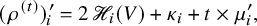 $$ \begin{align} (\rho^{(t)})_i^{\prime} = 2 \, \mathscr{H}_i (V) + \kappa_i + t \times \mu_i^{\prime}, \end{align} $$
 $$ \begin{align} (\lambda^{(t)})_i^{\prime} = 2 \, \mathscr{H}_i (V) + \kappa_i + (t+1) \times \mu_i^{\prime}. \end{align} $$
On the other hand, $\mathrm {odd}((\lambda ^{(1)})') + \mathrm {odd}((\rho ^{(1)})') = \mathrm {odd}((\lambda ^{(t)})') + \mathrm {odd}((\rho ^{(t)})')$
as a consequence of Proposition 10.4. This is because if
$\mathrm {odd}((\lambda ^{(1)})') + \mathrm {odd}((\rho ^{(1)})') = \mathrm {odd}((\lambda ^{(t)})') + \mathrm {odd}((\rho ^{(t)})')$
as a consequence of Proposition 10.4. This is because if
![]() , then
, then $\overline {\pi }$
and
$\overline {\pi }$
and $\overline {\pi }'$
have the same q and p words and their weights differ only by a constant shift, that is,
$\overline {\pi }'$
have the same q and p words and their weights differ only by a constant shift, that is, $w(\overline {\pi }')_i = w(\overline {\pi })_i+t-1$
for all i, implying
$w(\overline {\pi }')_i = w(\overline {\pi })_i+t-1$
for all i, implying $\mathrm {fixed}(\overline {\pi }) = \mathrm {fixed}(\overline {\pi }')$
. Combining these observations, we find
$\mathrm {fixed}(\overline {\pi }) = \mathrm {fixed}(\overline {\pi }')$
. Combining these observations, we find
 $$ \begin{align} \mathrm{odd}((\lambda^{(1)})') + \mathrm{odd}((\rho^{(1)})') = \mathrm{odd}(\kappa) + \mathrm{odd}(\kappa + \mu'), \end{align} $$
where the expression in the right-hand side is a result of checking parities of $\kappa _i,\mu _i^{\prime }$
and t in all cases.
$\kappa _i,\mu _i^{\prime }$
and t in all cases.
We now define functions
Lemma 10.6. For $k\ge 0$
, we have
$k\ge 0$
, we have
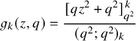
and
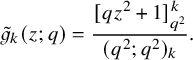
Proof. Any partition $\nu $
with first row of length k can be written as
$\nu $
with first row of length k can be written as $\nu '=\tilde {\nu }' + \eta (\varepsilon ;k)'$
where
$\nu '=\tilde {\nu }' + \eta (\varepsilon ;k)'$
where $\widetilde {\nu }$
has all even columns and first row
$\widetilde {\nu }$
has all even columns and first row $\widetilde {\nu }_1\le k$
and
$\widetilde {\nu }_1\le k$
and $\eta (\varepsilon ;k)$
is the partition defined by
$\eta (\varepsilon ;k)$
is the partition defined by
 $$ \begin{align} \eta(\varepsilon;k)^{\prime}_i-\eta(\varepsilon;k)^{\prime}_{i+1} = |\varepsilon_i - \varepsilon_{i+1}|, \qquad \text{for } i=1,\dots,k-1 \qquad\text{and}\qquad\eta(\varepsilon;k)_k^{\prime} = 2- \varepsilon_k, \end{align} $$
for $\varepsilon \in \{ 0,1\}^k$
. The binary sequence
$\varepsilon \in \{ 0,1\}^k$
. The binary sequence $\varepsilon $
encodes location of odd columns of
$\varepsilon $
encodes location of odd columns of $\nu $
. An example, for
$\nu $
. An example, for $k=6$
can be
$k=6$
can be
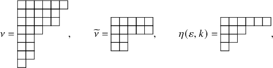
with $\varepsilon =(0,1,0,1,1,1)$
. Since by construction
$\varepsilon =(0,1,0,1,1,1)$
. Since by construction $\eta (\varepsilon ;k)_1=k$
, we can further decompose
$\eta (\varepsilon ;k)_1=k$
, we can further decompose $\eta (\varepsilon ;k)$
taking away one box from odd length columns and two boxes from even length columns, as
$\eta (\varepsilon ;k)$
taking away one box from odd length columns and two boxes from even length columns, as
 $$ \begin{align*}\eta(\varepsilon;k)' = 2 \widetilde{\eta}(\varepsilon;k)' + \varepsilon + 2(1-\varepsilon). \end{align*} $$
Notice that for fixed $j=|\varepsilon |=\varepsilon _1+\cdots +\varepsilon _k$
, we always have
$j=|\varepsilon |=\varepsilon _1+\cdots +\varepsilon _k$
, we always have $\widetilde {\eta }(\varepsilon ;k)^{\prime }_1\le j$
and
$\widetilde {\eta }(\varepsilon ;k)^{\prime }_1\le j$
and $\widetilde {\eta }(\varepsilon ;k)_1\le k$
. Moreover, for any partition
$\widetilde {\eta }(\varepsilon ;k)_1\le k$
. Moreover, for any partition $\lambda $
such that
$\lambda $
such that $\lambda _1\le k$
and
$\lambda _1\le k$
and $\lambda _1^{\prime } \le j$
, there always exists a choice of
$\lambda _1^{\prime } \le j$
, there always exists a choice of $\varepsilon $
such that
$\varepsilon $
such that $\widetilde {\eta }(\varepsilon ;k)=\lambda $
. Consider the generating function of Young diagrams
$\widetilde {\eta }(\varepsilon ;k)=\lambda $
. Consider the generating function of Young diagrams $\eta (\varepsilon ;k)$
 $$ \begin{align} \mathcal{Z}(\zeta,k) = \sum_{\varepsilon \in \{ 0,1 \}^k } \zeta^{ \, \mathrm{odd}(\eta(\varepsilon;k)')} q^{|\eta(\varepsilon;k)|} = \sum_{\varepsilon \in \{ 0,1 \}^k } (q \zeta)^{|\varepsilon|} q^{2(k-|\varepsilon|) + 2 \, |\widetilde{\eta}(\varepsilon;k)|}. \end{align} $$
By a notable combinatorial property of the Gaussian binomial coefficient [Reference Andrews, Askey and Roy2, Section 10], the right-hand side becomes, summing over fixed $|\varepsilon |$
,
$|\varepsilon |$
,
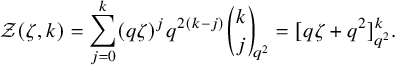 $$ \begin{align} \mathcal{Z}(\zeta,k) = \sum_{j=0}^k (q \zeta)^j q^{2(k-j)} \binom{k}{j}_{\hspace{-2pt} q^2} = [q \zeta + q^2]_{q^2}^k. \end{align} $$
Then the function
![]() becomes
becomes
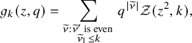
proving (10.22). Exact formula (10.23) easily follows from equation (10.22) by induction.
Lemma 10.7. For all $\mu $
, we have
$\mu $
, we have
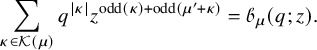
Proof. Summing over all different components of $\kappa = (\kappa ^{(1)},\kappa ^{(2)},\dots )$
and utilizing equation (10.23), we obtain the claimed result.
$\kappa = (\kappa ^{(1)},\kappa ^{(2)},\dots )$
and utilizing equation (10.23), we obtain the claimed result.
We finally come to the proof of equation (10.11).
Proof of Proposition 10.3.
By making use of computation reported in Proposition 10.7, we obtain
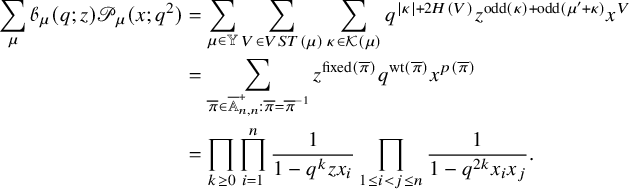
Remark 10.8. Identities (10.3), (10.11) hold both numerically and formally in the algebra of symmetric functions. In this second case, variables x can be thought as generic algebra homomorphisms defined on the (algebraic) basis of power sum symmetric functions $\{p_n;n\in \mathbb {N}_0 \}$
as
$\{p_n;n\in \mathbb {N}_0 \}$
as
 $$ \begin{align} x : p_n \mapsto x (p_n). \end{align} $$
Remark 10.9. It is known [Reference Macdonald62] that the algebra homomorphism
 $$ \begin{align} \omega_{u,v} : p_r \mapsto (-1)^{r-1} \frac{1 - u^r}{1-v^r} p_r \end{align} $$
acts on Macdonald polynomials $\mathscr {P}_{\mu }(x;q,t),\mathscr {Q}_{\mu }(x;q,t)$
as
$\mathscr {P}_{\mu }(x;q,t),\mathscr {Q}_{\mu }(x;q,t)$
as
 $$ \begin{align} \omega_{q,t} \mathscr{P}_{\mu} (x;q,t) = \mathscr{Q}_{\mu'}(x, t, q). \end{align} $$
Then, applying $\omega _{q^2,0}$
to both sides of equation (10.11) and renaming parameters
$\omega _{q^2,0}$
to both sides of equation (10.11) and renaming parameters $q \mapsto t$
yields the identity for Hall–Littlewood polynomials
$q \mapsto t$
yields the identity for Hall–Littlewood polynomials $\mathscr {Q}_{\mu }(x;q=0,t)$
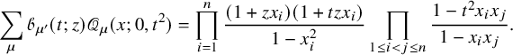
This identity is a particular case of [Reference Warnaar91, Theorem 1.1], which in turn interpolates between one of Macdonald’s Littlewood identities [Reference Macdonald62] and Kawanaka’s Littlewood identity [Reference Kawanaka52].
Remark 10.10. In this paper, we have focused our attention on q-Whittaker polynomials, which naturally arise as generating functions of vertically strict tableaux. Following the recipe outlined in Section 8.3, it should be possible to study bijectively summation identities involving modified Hall–Littlewood polynomials $\mathscr {Q}^{\prime }_{\mu }(x;q)$
; see [Reference Désarménien, Leclerc and Thibon25] for a review. They can be defined as a generating function of row weak tableaux of fixed shape and weighted by a suitable adaptation of the intrinsic energy function [Reference Nakayashiki and Yamada65].
$\mathscr {Q}^{\prime }_{\mu }(x;q)$
; see [Reference Désarménien, Leclerc and Thibon25] for a review. They can be defined as a generating function of row weak tableaux of fixed shape and weighted by a suitable adaptation of the intrinsic energy function [Reference Nakayashiki and Yamada65].
10.2 Identities between summations of q-Whittaker and skew Schur functions
The bijection presented in Proposition 8.1, along with generalization of Schensted’s theorem of Proposition 6.7, reveal correspondences between certain summations of q-Whittaker polynomials and skew Schur polynomials. For partitions $\rho \subseteq \lambda $
, define the skew Schur polynomial [Reference Macdonald62] in n variables
$\rho \subseteq \lambda $
, define the skew Schur polynomial [Reference Macdonald62] in n variables $x=(x_1,\dots , x_n)$
as
$x=(x_1,\dots , x_n)$
as
 $$ \begin{align} s_{\lambda/\rho} (x) = \sum_{P \in SST(\lambda/\rho,n)} x^P. \end{align} $$
The following theorem was first proved in [Reference Imamura, Mucciconi and Sasamoto44] using methods coming from integrable probability. Here, we give its bijective proof.
Theorem 10.11. Fix $|q|<1$
, and set of variables
$|q|<1$
, and set of variables $x=(x_1,\dots ,x_n)$
,
$x=(x_1,\dots ,x_n)$
, $y=(y_1,\dots ,y_n)$
. Then, for all
$y=(y_1,\dots ,y_n)$
. Then, for all $k=0,1,2,\dots $
, we have
$k=0,1,2,\dots $
, we have

Proof. The right-hand side of equation (10.36) can be written, by means of bijection of Proposition 8.1 and Proposition 6.7, as
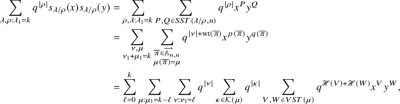 $$ \begin{align} \begin{aligned} \sum_{\lambda,\rho : \lambda_1= k} q^{|\rho|} s_{\lambda / \rho}(x) s_{\lambda / \rho}(y)&= \sum_{\rho, \lambda: \lambda_1=k}\sum_{P,Q\in SST(\lambda/\rho,n) } q^{|\rho|} x^P y^Q \\ &=\sum_{\substack{\nu,\mu \\ \nu_1+\mu_1=k}} \sum_{\substack{\overline{\pi} \in \overline{\mathbb{A}}_{n,n}^+ \\ \mu(\overline{\pi}) = \mu } }q^{|\nu| + \mathrm{wt}(\overline{\pi})} x^{p(\overline{\pi})} y^{q(\overline{\pi})} \\&= \sum_{\ell=0}^k \sum_{\mu:\mu_1=k-\ell} \sum_{\nu: \nu_1=\ell} q^{|\nu|} \sum_{\kappa \in \mathcal{K}(\mu)} q^{|\kappa|} \sum_{V,W\in VST(\mu)} q^{\mathscr{H}(V) + \mathscr{H}(W)} x^{V} y^{W}, \end{aligned} \end{align} $$
which reduces to the left-hand side after putting all summations in closed form.
Imposing a symmetry to our bijection, we can easily prove the following additional identity.
Theorem 10.12. Fix $|q|<1$
, and set of variables
$|q|<1$
, and set of variables $x=(x_1,\dots ,x_n)$
. Then, recalling notation (10.8), (10.22), we have
$x=(x_1,\dots ,x_n)$
. Then, recalling notation (10.8), (10.22), we have
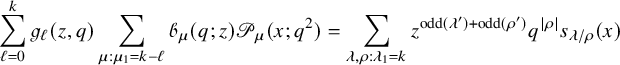
for all $k=0,1,2,\dots $
.
$k=0,1,2,\dots $
.
Proof. Using Proposition 10.4, Proposition 10.5 and the bijection of Proposition 8.1, the right-hand side of equation (10.38) can be written as
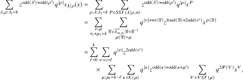 $$ \begin{align*} \begin{aligned} \sum_{\lambda,\rho : \lambda_1= k} z^{\mathrm{odd}(\lambda') + \mathrm{odd}(\rho')} q^{|\rho|} s_{\lambda / \rho}(x) &= \sum_{\rho,\lambda:\lambda_1=k} \sum_{P\in SST(\lambda/\rho,n)} z^{\mathrm{odd}(\lambda') + \mathrm{odd}(\rho')} q^{|\rho|} x^P \\ &=\sum_{\substack{\nu,\mu \\ \nu_1+\mu_1=k}} \sum_{\substack{\overline{\pi} \in \overline{\mathbb{A}}_{n,n}^+: \overline{\pi} = \overline{\pi}^{-1} \\ \mu(\overline{\pi}) = \mu } } q^{|\nu| + \mathrm{wt}(\overline{\pi})} z^{\mathrm{fixed}(\overline{\pi}) + 2\mathrm{odd}(\nu')} x^{p(\overline{\pi})} \\ &= \sum_{\ell=0}^k \sum_{\nu: \nu_1=\ell} q^{|\nu|} z^{2\mathrm{odd}(\nu')} \\ & \qquad \times\sum_{\mu:\mu_1=k-\ell} \sum_{\kappa \in \mathcal{K}(\mu)} q^{|\kappa|} z^{\mathrm{odd}(\kappa)+\mathrm{odd}(\kappa + \mu')} \sum_{V\in VST(\mu)} q^{2\mathscr{H}(V)} x^{V}, \end{aligned} \end{align*} $$
which reduces to the left-hand side after using equation (10.22), Proposition 10.7.
Remark 10.13. Identities stated in Propositions 10.11 and 10.12 can be further refined taking advantage of homogeneity of q-Whittaker and skew Schur polynomials. For instance, for any fixed $k,N=0,1,2,\dots $
, we have
$k,N=0,1,2,\dots $
, we have
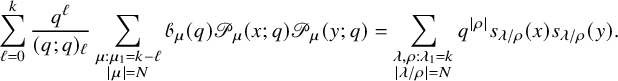
A similar refinement can be given for equation (10.38), fixing the degree N of polynomials in the left- and right-hand sides.
Remark 10.14. Just as discussed in Proposition 10.8, also identities (10.36), (10.38) hold both numerically and formally in the algebra of symmetric function. They are therefore still true if variables x are replaced by algebra homomorphisms $x:p_n\mapsto x(p_n)$
. An application of this fact is that, through the action of
$x:p_n\mapsto x(p_n)$
. An application of this fact is that, through the action of $\omega _{q^2,0}$
, equations (10.36), (10.38) turn into summation identities relating Hall–Littlewood symmetric polynomials
$\omega _{q^2,0}$
, equations (10.36), (10.38) turn into summation identities relating Hall–Littlewood symmetric polynomials $\mathscr {P}_{\mu }(x,q=0,t)$
and Schur functions. This fact has deep consequences in the context of stochastic solvable models related to q-Whittaker and Hall–Littlewood symmetric polynomials (see [Reference Barraquand, Borodin and Corwin7, Reference Barraquand, Borodin, Corwin and Wheeler8, Reference Borodin, Bufetov and Wheeler13, Reference Borodin and Corwin14, Reference Vuletic90], and we will investigate these aspects in a forthcoming paper [Reference Imamura, Mucciconi and Sasamoto45]).
$\mathscr {P}_{\mu }(x,q=0,t)$
and Schur functions. This fact has deep consequences in the context of stochastic solvable models related to q-Whittaker and Hall–Littlewood symmetric polynomials (see [Reference Barraquand, Borodin and Corwin7, Reference Barraquand, Borodin, Corwin and Wheeler8, Reference Borodin, Bufetov and Wheeler13, Reference Borodin and Corwin14, Reference Vuletic90], and we will investigate these aspects in a forthcoming paper [Reference Imamura, Mucciconi and Sasamoto45]).
A Knuth relations and generalizations
A.1 Knuth equivalence and jeu de taquin
In this subsection, we cover some prerequisites on the theories of Knuth relations and jeu de taquin and on their interplay. The material presented here is standard, and for more detailed expositions on the topic we suggest the interested reader to consult textbooks as [Reference Lothaire60, Reference Sagan74].
Following [Reference Knuth54], on the set of words $\mathcal {A}_n^*$
we define the Knuth relation
$\mathcal {A}_n^*$
we define the Knuth relation $\pi \simeq \pi '$
as the equivalence relation generated by the transformations
$\pi \simeq \pi '$
as the equivalence relation generated by the transformations
 $$ \begin{align} \alpha \, x \, z \, y \, \beta \rightleftharpoons \alpha \,z \, x \, y \, \beta \hspace{.4cm} \text{if } x\le y < z, \hspace{.4cm} \text{and} \hspace{.4cm} \alpha \, y \, z \, x \, \beta \rightleftharpoons \alpha \, y \, x \,z \, \beta, \hspace{.4cm} \text{if } x < y \le z, \end{align} $$
where $\alpha ,\beta $
are generic words. These are often called elementary transformations or Knuth moves. In practice, they represent a realization in the language of words of the Schensted’s insertion of a letter in a row of a tableau. To explain this analogy, take a word
$\alpha ,\beta $
are generic words. These are often called elementary transformations or Knuth moves. In practice, they represent a realization in the language of words of the Schensted’s insertion of a letter in a row of a tableau. To explain this analogy, take a word $w=w_1\cdots w_k$
with letters in weakly increasing order
$w=w_1\cdots w_k$
with letters in weakly increasing order $w_1 \le \cdots \le w_k$
, which we can interpret as a word formed reading a row of a semistandard tableau. Then, for any
$w_1 \le \cdots \le w_k$
, which we can interpret as a word formed reading a row of a semistandard tableau. Then, for any $x < w_k$
we have, applying equation (A.1) repeatedly,
$x < w_k$
we have, applying equation (A.1) repeatedly,
 $$ \begin{align} wx \simeq x^* w^*, \end{align} $$
where $x^*$
is the smallest
$x^*$
is the smallest $w_i$
to be strictly bigger than x and
$w_i$
to be strictly bigger than x and $w^*$
is the word obtained from w substituting
$w^*$
is the word obtained from w substituting $x^*$
with x. On the other hand, if
$x^*$
with x. On the other hand, if $x \ge w_k$
, then no Knuth moves can be applied to transform the word
$x \ge w_k$
, then no Knuth moves can be applied to transform the word $w^*=wx$
. We see that in both cases
$w^*=wx$
. We see that in both cases $w^*$
is the row word after the insertion of x, and when
$w^*$
is the row word after the insertion of x, and when $x<w_k$
, the letter
$x<w_k$
, the letter $x^*$
will be the one inserted in the following row. This idea motivates the characterization of Knuth equivalence classes.
$x^*$
will be the one inserted in the following row. This idea motivates the characterization of Knuth equivalence classes.
Theorem A.1 ([Reference Sagan74] Theorem 3.4.3).
Two words $\pi ,\pi '$
are equivalent if and only if their P-tableaux under RSK correspondence is equal
$\pi ,\pi '$
are equivalent if and only if their P-tableaux under RSK correspondence is equal $P(\pi )=P(\pi ')$
.
$P(\pi )=P(\pi ')$
.
The notion of Knuth equivalence extends also at the level of skew shaped semistandard tableaux. We say that two tableaux P and $P'$
are Knuth equivalent or simply equivalent if their row reading words
$P'$
are Knuth equivalent or simply equivalent if their row reading words $w_P$
and
$w_P$
and $w_{P'}$
are, in which case we write
$w_{P'}$
are, in which case we write $P \simeq P'$
. Equivalent tableaux enjoy the property that they can be transformed into each other through the procedure of jeu de taquin. This operation is described in terms of sliding moves. We say that a semistandard tableau P is punctured if we replace the entry of one or more of its cells with the symbol
$P \simeq P'$
. Equivalent tableaux enjoy the property that they can be transformed into each other through the procedure of jeu de taquin. This operation is described in terms of sliding moves. We say that a semistandard tableau P is punctured if we replace the entry of one or more of its cells with the symbol $\bullet $
. From a punctured tableau P, we can remove the
$\bullet $
. From a punctured tableau P, we can remove the $\bullet $
-cells as follows. Assume that cells
$\bullet $
-cells as follows. Assume that cells $(i,j),(i+1,j)$
and
$(i,j),(i+1,j)$
and $(i,j+1)$
have, respectively, entries
$(i,j+1)$
have, respectively, entries $\bullet , a$
and b. Then if
$\bullet , a$
and b. Then if $a \le b$
, we exchange the labels of cells
$a \le b$
, we exchange the labels of cells $(i,j)$
and
$(i,j)$
and $(i+1,j)$
, while if
$(i+1,j)$
, while if $a>b$
we swap the labels at
$a>b$
we swap the labels at $(i,j)$
and
$(i,j)$
and $(i,j+1)$
. This single move is the inward sliding, and graphically we have
$(i,j+1)$
. This single move is the inward sliding, and graphically we have
When either cell $(i+1,j)$
or
$(i+1,j)$
or $(i,j+1)$
is not part of the shape of the tableaux, we think of their value as infinite, while when the
$(i,j+1)$
is not part of the shape of the tableaux, we think of their value as infinite, while when the $\bullet $
-cell reaches an external corner we simply erase it. From a tableau P of shape
$\bullet $
-cell reaches an external corner we simply erase it. From a tableau P of shape $\lambda /\mu $
, let c be an external corner of
$\lambda /\mu $
, let c be an external corner of $\mu $
. The outward jeu de taquin
$\mu $
. The outward jeu de taquin $J_{c}(P)$
is the tableau obtained puncturing the cell c of P and sliding out the
$J_{c}(P)$
is the tableau obtained puncturing the cell c of P and sliding out the $\bullet $
-cell.
$\bullet $
-cell.
The sliding moves can be also defined in the opposite direction, moving the $\bullet $
-cells inwards. If in a punctured tableaux the cells
$\bullet $
-cells inwards. If in a punctured tableaux the cells $(i,j), (i,j-1)$
and
$(i,j), (i,j-1)$
and $(i-1,j)$
have labels
$(i-1,j)$
have labels $\bullet , a$
and b, we will slide b up in case
$\bullet , a$
and b, we will slide b up in case $a\le b$
, while a is shifted rightward when
$a\le b$
, while a is shifted rightward when $a> b$
, as in
$a> b$
, as in
After a number of inward slides, the $\bullet $
-cell will reach an inner corner and in that case it is erased. This procedure defines inward jeu de taquin transformations. If P is a skew tableau of shape
$\bullet $
-cell will reach an inner corner and in that case it is erased. This procedure defines inward jeu de taquin transformations. If P is a skew tableau of shape $\lambda /\mu $
and
$\lambda /\mu $
and $c\notin \lambda $
is such that
$c\notin \lambda $
is such that $c-\mathbf {e}_1,c-\mathbf {e}_2 \in \lambda $
, then
$c-\mathbf {e}_1,c-\mathbf {e}_2 \in \lambda $
, then $J_c(P)$
is the tableau obtained from P puncturing the cell c and sliding inward the
$J_c(P)$
is the tableau obtained from P puncturing the cell c and sliding inward the $\bullet $
-cell. We do not differentiate the notation between inward and outward jeu de taquin as the choice of the cell c dictates the direction of sliding.
$\bullet $
-cell. We do not differentiate the notation between inward and outward jeu de taquin as the choice of the cell c dictates the direction of sliding.
The jeu de taquin can be employed to associate to skew-shaped semistandard tableaux canonical straight shaped ones. Given a tableau P of shape $\lambda / \mu $
, we fill the empty shape
$\lambda / \mu $
, we fill the empty shape $\mu $
with
$\mu $
with $\bullet $
-cells and subsequently we slide them all out. The result is a tableaux of straight shape
$\bullet $
-cells and subsequently we slide them all out. The result is a tableaux of straight shape $\widetilde {\lambda }$
called jeu de taquin rectification of P and denoted as
$\widetilde {\lambda }$
called jeu de taquin rectification of P and denoted as $\mathrm {rect}(P)$
. It is a theorem of Schützenberger [Reference Sagan74, Theorem 3.7.7] that the rectification is independent of the order of sliding moves.
$\mathrm {rect}(P)$
. It is a theorem of Schützenberger [Reference Sagan74, Theorem 3.7.7] that the rectification is independent of the order of sliding moves.
The following classical theorem states the relation between Knuth equivalence of tableaux and jeu de taquin.
Theorem A.2 ([Reference Schützenberger78],[Reference Sagan74] Theorem 3.7.8).
Two tableaux $P,P'$
are equivalent if and only if their jeu de taquin rectification is equal. In particular,
$P,P'$
are equivalent if and only if their jeu de taquin rectification is equal. In particular, $P \simeq P'$
if and only if they can be transformed into each other through a finite sequence of jeu de taquin moves.
$P \simeq P'$
if and only if they can be transformed into each other through a finite sequence of jeu de taquin moves.
Remark A.3. An equivalent definition of the Knuth equivalence between tableaux $P,P'$
can be given requiring that their column reading words
$P,P'$
can be given requiring that their column reading words $w^{\mathrm {col}}_P \simeq w^{\mathrm {col}}_{P'}$
. More in general, in [Reference Fomin and Greene28] the authors discuss a full class or reading orders for tableaux, which include row and column ones, producing equivalent theories of Knuth equivalence.
$w^{\mathrm {col}}_P \simeq w^{\mathrm {col}}_{P'}$
. More in general, in [Reference Fomin and Greene28] the authors discuss a full class or reading orders for tableaux, which include row and column ones, producing equivalent theories of Knuth equivalence.
We close this subsection stating several simple but crucial properties that endow the skew $\mathbf {RSK}$
map with its many symmetries.
$\mathbf {RSK}$
map with its many symmetries.
Proposition A.4. Let P be a semistandard skew tableau and $P' = \mathcal {R}_{[r]}(P)$
for some row r. Then
$P' = \mathcal {R}_{[r]}(P)$
for some row r. Then $P \simeq P'$
.
$P \simeq P'$
.
Proof. The tableau $P'$
is obtained from P vacating the leftmost cell at row r and inserting the entry of the vacated cell in the row below. The fact that the insertion algorithm is reproduced at the level of row words by a sequence of Knuth moves yields the proof.
$P'$
is obtained from P vacating the leftmost cell at row r and inserting the entry of the vacated cell in the row below. The fact that the insertion algorithm is reproduced at the level of row words by a sequence of Knuth moves yields the proof.
Proposition A.5. Let $P,Q$
be semistandard tableaux with same skew shape and take
$P,Q$
be semistandard tableaux with same skew shape and take $(P',Q')=\mathbf {RSK}(P,Q)$
. Then
$(P',Q')=\mathbf {RSK}(P,Q)$
. Then $P \simeq P'$
and
$P \simeq P'$
and $Q \simeq Q'$
.
$Q \simeq Q'$
.
Proof. By the result stated in Proposition 3.6 $P'$
and
$P'$
and $Q'$
are obtained, respectively, from P and Q after a sequence of internal insertions. Then, by Proposition A.4, we have
$Q'$
are obtained, respectively, from P and Q after a sequence of internal insertions. Then, by Proposition A.4, we have $P\simeq P'$
and
$P\simeq P'$
and $Q\simeq Q'$
.
$Q\simeq Q'$
.
Proposition A.6. Let $\overline {\pi }\in \overline {\mathbb {A}}_{n,n}$
, and consider the pair of tableaux
$\overline {\pi }\in \overline {\mathbb {A}}_{n,n}$
, and consider the pair of tableaux
![]() , for some partition
, for some partition $\nu $
. Define
$\nu $
. Define
![]() and
and
![]() . Then
. Then
 $$ \begin{align} P \simeq P(\pi') \qquad \text{and} \qquad Q \simeq P(\pi"). \end{align} $$
Proof. From the definition of the Sagan–Stanley correspondence, we understand that the timetable ordering
![]() records the‘times’ at which each entry of the P tableau is inserted in its first row. More precisely, the word
records the‘times’ at which each entry of the P tableau is inserted in its first row. More precisely, the word
![]() is the list of such entries in order of insertion. By Proposition A.4,
is the list of such entries in order of insertion. By Proposition A.4, $\pi '$
is Knuth equivalent to the row word of P and therefore
$\pi '$
is Knuth equivalent to the row word of P and therefore $P \simeq P(\pi ')$
. The alternative statement for the Q tableau is proven analogously using the swap symmetry of Proposition A.4.
$P \simeq P(\pi ')$
. The alternative statement for the Q tableau is proven analogously using the swap symmetry of Proposition A.4.
A.2 Dual equivalence
Two words $\pi , \pi '$
are dual equivalent if their Q-tableaux under RSK correspondence are equal. We denote dual equivalence by
$\pi , \pi '$
are dual equivalent if their Q-tableaux under RSK correspondence are equal. We denote dual equivalence by $\pi \stackrel {*}{\simeq } \pi '$
. We say that two skew tableaux
$\pi \stackrel {*}{\simeq } \pi '$
. We say that two skew tableaux $P,P'$
of the same shape are dual equivalent if their column reading words are dual equivalen,t and in this case, we write
$P,P'$
of the same shape are dual equivalent if their column reading words are dual equivalen,t and in this case, we write $P \stackrel {*}{\simeq } P'$
. Again, by a result of [Reference Fomin and Greene28], the notion of dual equivalence does not depend on the reading order of the tableaux and in literature often the row reading is used. The theory of dual equivalence was started by Haiman in [Reference Haiman39], and below we present two classical results that will be relevant to us.
$P \stackrel {*}{\simeq } P'$
. Again, by a result of [Reference Fomin and Greene28], the notion of dual equivalence does not depend on the reading order of the tableaux and in literature often the row reading is used. The theory of dual equivalence was started by Haiman in [Reference Haiman39], and below we present two classical results that will be relevant to us.
Theorem A.7 ([Reference Haiman39],[Reference Sagan74] Theorem 3.8.8).
Two tableaux $P_1,P_2$
are dual equivalent if and only if for any sequence of jeu de taquin slides J the tableaux
$P_1,P_2$
are dual equivalent if and only if for any sequence of jeu de taquin slides J the tableaux $J(P_1), J(P_2)$
have the same shape.
$J(P_1), J(P_2)$
have the same shape.
Theorem A.8 ([Reference Haiman39] Theorem 2.13).
Let $P,P'$
be two semistandard tableaux with same skew shape. Then
$P,P'$
be two semistandard tableaux with same skew shape. Then $P\simeq P'$
and
$P\simeq P'$
and $P \stackrel {*}{\simeq } P'$
if and only if
$P \stackrel {*}{\simeq } P'$
if and only if $P=P'$
.
$P=P'$
.
In the following theorem, we use the notion of Kashiwara operators defined in Section 5.2.
Theorem A.9 ([Reference Lothaire60], Theorem 5.5.1).
Let h be anyone between $\widetilde {e}_{i},\widetilde {f}_{i},i=1,\dots ,n-1$
and
$\widetilde {e}_{i},\widetilde {f}_{i},i=1,\dots ,n-1$
and $\pi \in \mathcal {A}_n^*$
such that
$\pi \in \mathcal {A}_n^*$
such that $h(\pi ) \neq \varnothing $
. Then
$h(\pi ) \neq \varnothing $
. Then
-
1.
$h(\pi ) \stackrel {*}{\simeq } \pi $
; -
2. if
$\pi ' \simeq \pi $
then
$h(\pi ') \simeq h(\pi )$
.


A.3 Generalized Knuth relations for weighted words
We recall that a weighted word is just a weighted biword $\overline {\pi }$
having q-word
$\overline {\pi }$
having q-word $q(\overline {\pi })=q_1q_2 \cdots q_k=12 \cdots k$
, where k is the length of
$q(\overline {\pi })=q_1q_2 \cdots q_k=12 \cdots k$
, where k is the length of $\overline {\pi }$
. Borrowing a notation used in [Reference Sagan and Stanley73], we will write such a
$\overline {\pi }$
. Borrowing a notation used in [Reference Sagan and Stanley73], we will write such a $\overline {\pi }$
as a word in the weighted alphabet
$\overline {\pi }$
as a word in the weighted alphabet $\overline {\mathcal {A}}_n$
consisting of symbols
$\overline {\mathcal {A}}_n$
consisting of symbols $a^{(w)}$
, where
$a^{(w)}$
, where $a\in \{1,\dots ,n\}$
and
$a\in \{1,\dots ,n\}$
and $w\in \mathbb {Z}$
. In this more compact notation, for instance, we write
$w\in \mathbb {Z}$
. In this more compact notation, for instance, we write
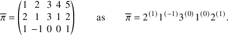 $$ \begin{align} \overline{\pi}= \left( \begin{matrix} 1 & 2 & 3 & 4 & 5 \\ 2 & 1 & 3 & 1 & 2 \\ 1 & -1 & 0 & 0 & 1 \end{matrix} \right) \qquad \text{as} \qquad \overline{\pi}= 2^{(1)} 1^{(-1)} 3^{(0)} 1^{(0)} 2^{(1)}. \end{align} $$
On $\overline {\mathcal {A}}_n$
, we introduce the total ordering
$\overline {\mathcal {A}}_n$
, we introduce the total ordering $\prec $
defined as
$\prec $
defined as
 $$ \begin{align} a^{(w)} \prec b^{(w')} \qquad \text{if} \quad w> w', \qquad \text{or} \quad w=w' , a< b. \end{align} $$
The following definition generalizes the classical Knuth relations recalled in equation (A.1).
Definition A.10 (Generalized Knuth relations).
The generalized Knuth relations $\overline {\pi } \simeq _{\mathrm {g}} \overline {\pi }'$
is the equivalence relation on weighted words generated by the transformations
$\overline {\pi } \simeq _{\mathrm {g}} \overline {\pi }'$
is the equivalence relation on weighted words generated by the transformations
 $$ \begin{align} \begin{aligned} \alpha \, x^{(w_x)} \, z^{(w_z)} \, y^{(w_y)} \, \beta \rightleftharpoons \alpha \,z^{(w_z)} \, x^{(w_x)} \, y^{(w_y)} \, \beta, \qquad &\text{if } x^{(w_x)} \preceq y^{(w_y)} \prec z^{(w_z)}, \\ \alpha \, y^{(w_y)} \, z^{(w_z)} \, x^{(w_x)} \, \beta \rightleftharpoons \alpha \, y^{(w_y)} \, z^{(w_z)} \,x^{(w_x)} \, \beta, \qquad &\text{if } x^{(w_x)} \prec y^{(w_y)} \preceq z^{(w_z)},\end{aligned} \end{align} $$
where $\alpha ,\beta $
are generic weighted words. If a transformation swaps the i-th and the
$\alpha ,\beta $
are generic weighted words. If a transformation swaps the i-th and the $i+1$
-th letter of a weighted word, we say that such transformation has type i. For a graphical interpretation of equation (A.6), see Figure 22.
$i+1$
-th letter of a weighted word, we say that such transformation has type i. For a graphical interpretation of equation (A.6), see Figure 22.
Representing weighted words as point configurations on the twisted cylinder $\mathscr {C}_n$
, the two relations (A.6) correspond, respectively, to the left and right panels above.
$\mathscr {C}_n$
, the two relations (A.6) correspond, respectively, to the left and right panels above.
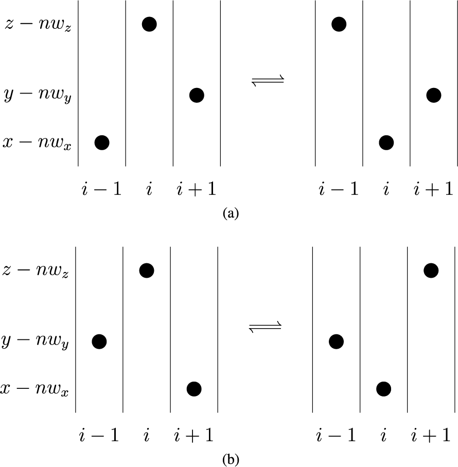
The following theorem offers a characterization of generalized Knuth equivalence classes, that partially extends Proposition A.1. Given a weighted biword $\overline {\pi }$
, we denote with
$\overline {\pi }$
, we denote with $(P_t(\overline {\pi }),Q_t(\overline {\pi }))$
the skew
$(P_t(\overline {\pi }),Q_t(\overline {\pi }))$
the skew $\mathbf {RSK}$
dynamics with initial data
$\mathbf {RSK}$
dynamics with initial data $(P,Q)\xrightarrow []{\mathbf {SS}\,}\overline {\pi }$
.
$(P,Q)\xrightarrow []{\mathbf {SS}\,}\overline {\pi }$
.
Theorem A.11. Consider a pair of weighted words $\overline {\pi } \simeq _{\mathrm {g}} \overline {\pi }'$
. Then for all
$\overline {\pi } \simeq _{\mathrm {g}} \overline {\pi }'$
. Then for all $t \in \mathbb {Z}$
, we have
$t \in \mathbb {Z}$
, we have $P_t(\overline {\pi }) = P_t(\overline {\pi }')$
.
$P_t(\overline {\pi }) = P_t(\overline {\pi }')$
.
The proof of Proposition A.11 is based on a simple quasi-commutation relation between Knuth relations and the Viennot map.
Lemma A.12. Let $\overline {\pi }$
and
$\overline {\pi }$
and $\overline {\pi }'$
be weighted permutations differing by a single Knuth transformation of type i. Then
$\overline {\pi }'$
be weighted permutations differing by a single Knuth transformation of type i. Then $\mathbf {V}(\overline {\pi })$
and
$\mathbf {V}(\overline {\pi })$
and $\mathbf {V}(\overline {\pi }')$
also differ by a single Knuth transformation whose type is either
$\mathbf {V}(\overline {\pi }')$
also differ by a single Knuth transformation whose type is either $i-1$
, i or
$i-1$
, i or $i+1$
.
$i+1$
.
Proof. Our statement is best proven through a graphical argument. In equations (A.7), (A.8), (A.9), we give a schematic representation of all possible cases that could present while performing a generalized Knuth transformation. We focus only on the sector $\mathsf {S}_{i,i+2}=\{i,i+1,i+2\} \times \mathbb {Z} \subseteq \mathscr {C}_n$
where the transformation that takes place as the remaining part of the construction is determined by unaffected points outside
$\mathsf {S}_{i,i+2}=\{i,i+1,i+2\} \times \mathbb {Z} \subseteq \mathscr {C}_n$
where the transformation that takes place as the remaining part of the construction is determined by unaffected points outside $\mathsf {S}_{i,i+2}$
and by the heights
$\mathsf {S}_{i,i+2}$
and by the heights $j_1,j_2,j_3$
and
$j_1,j_2,j_3$
and $j_1^{\prime },j_2^{\prime },j_3^{\prime }$
of the horizontal segments originating and terminating inside
$j_1^{\prime },j_2^{\prime },j_3^{\prime }$
of the horizontal segments originating and terminating inside $\mathsf {S}_{i,i+2}$
. In equations (A.7), (A.8), we show the cases where the first transformation of equation (A.6) is applied
$\mathsf {S}_{i,i+2}$
. In equations (A.7), (A.8), we show the cases where the first transformation of equation (A.6) is applied
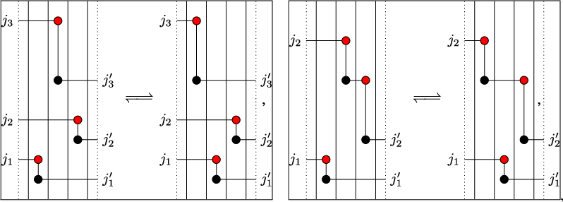
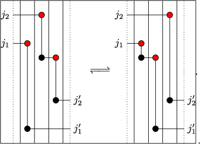
The cases where the second transformation of equation (A.6) is applied are shown below:
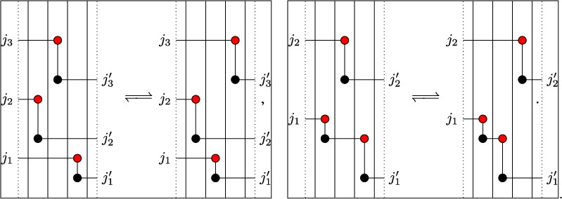
In all cases, except for equation (A.8), the generalized Knuth transformation separating $\mathbf {V}(\overline {\pi })$
and
$\mathbf {V}(\overline {\pi })$
and $\mathbf {V}(\overline {\pi }')$
is the same separating
$\mathbf {V}(\overline {\pi }')$
is the same separating $\overline {\pi }$
and
$\overline {\pi }$
and $\overline {\pi }'$
. The only nontrivial assumption made in the figures above is that the heights
$\overline {\pi }'$
. The only nontrivial assumption made in the figures above is that the heights $j_1,j_2,j_3$
of shadow lines entering the sector
$j_1,j_2,j_3$
of shadow lines entering the sector $\mathsf {S}_{i,i+2}$
are not affected by the transformations. This is a consequence of the fact that the position of horizontal lines exiting
$\mathsf {S}_{i,i+2}$
are not affected by the transformations. This is a consequence of the fact that the position of horizontal lines exiting $\mathsf {S}_{i,i+2}$
at heights
$\mathsf {S}_{i,i+2}$
at heights $j_1^{\prime },j_2^{\prime },j_3^{\prime }$
also does not change while swapping the highest and lowest point of the triple.
$j_1^{\prime },j_2^{\prime },j_3^{\prime }$
also does not change while swapping the highest and lowest point of the triple.
Proof of Proposition A.11.
It is sufficient to prove this theorem in case $\overline {\pi }$
is a weighted permutation as this result would extend to weighted words via standardization. We show that if
$\overline {\pi }$
is a weighted permutation as this result would extend to weighted words via standardization. We show that if $\overline {\pi }$
and
$\overline {\pi }$
and $\overline {\pi }'$
are separated by a single generalized Knuth relation then
$\overline {\pi }'$
are separated by a single generalized Knuth relation then $P_t(\overline {\pi }) = P_t(\overline {\pi }')$
for all t. We recall that
$P_t(\overline {\pi }) = P_t(\overline {\pi }')$
for all t. We recall that $P_t(\overline {\pi })$
is obtained reading values of east edges
$P_t(\overline {\pi })$
is obtained reading values of east edges $\mathsf {E}(n,n(t-1)+1),\dots ,\mathsf {E}(n,nt)$
of the edge configuration
$\mathsf {E}(n,n(t-1)+1),\dots ,\mathsf {E}(n,nt)$
of the edge configuration $\mathcal {E}(\overline {\pi })$
. On the other hand, if
$\mathcal {E}(\overline {\pi })$
. On the other hand, if $\{\overline {\pi }^{(t)}\}_t$
is the Viennot dynamics with initial data
$\{\overline {\pi }^{(t)}\}_t$
is the Viennot dynamics with initial data $\overline {\pi }^{(1)}=\overline {\pi }$
, then
$\overline {\pi }^{(1)}=\overline {\pi }$
, then $\mathcal {E}(\overline {\pi })$
is completely determined by the shadow line constructions of transitions
$\mathcal {E}(\overline {\pi })$
is completely determined by the shadow line constructions of transitions $\overline {\pi }^{(t)} \to \overline {\pi }^{(t+1)}$
. In fact, the segments of each shadow line construction determine all edges having a same fixed value. By arguments presented in the proof of Proposition A.12, if the Knuth transformation
$\overline {\pi }^{(t)} \to \overline {\pi }^{(t+1)}$
. In fact, the segments of each shadow line construction determine all edges having a same fixed value. By arguments presented in the proof of Proposition A.12, if the Knuth transformation $\overline {\pi }\to \overline {\pi }'$
involves
$\overline {\pi }\to \overline {\pi }'$
involves $i,i+1$
and
$i,i+1$
and $i+2$
-th letters of both weighted permutations, then this is also the case for
$i+2$
-th letters of both weighted permutations, then this is also the case for $\mathbf {V}(\overline {\pi }) \to \mathbf {V} (\overline {\pi }')$
. Moreover, the shadow line construction is unaffected at columns different than
$\mathbf {V}(\overline {\pi }) \to \mathbf {V} (\overline {\pi }')$
. Moreover, the shadow line construction is unaffected at columns different than $i,i+1,i+2$
. This implies that edge configurations
$i,i+1,i+2$
. This implies that edge configurations $\mathcal {E}(\overline {\pi })$
and
$\mathcal {E}(\overline {\pi })$
and $\mathcal {E}(\overline {\pi }')$
differ only at edges corresponding to columns
$\mathcal {E}(\overline {\pi }')$
differ only at edges corresponding to columns $i,i+1,i+2$
and moreover east edges
$i,i+1,i+2$
and moreover east edges $\mathsf {E}(n,j)$
are common for all j. This concludes the proof.
$\mathsf {E}(n,j)$
are common for all j. This concludes the proof.
Remark A.13. It is easy to see that if two weighted words $\overline {\pi }$
and
$\overline {\pi }$
and $\overline {\pi }'$
have the same P tableaux under Sagan–Stanley correspondence, then they are not necessarily connected by a sequence of generalized Knuth relations. For example,
$\overline {\pi }'$
have the same P tableaux under Sagan–Stanley correspondence, then they are not necessarily connected by a sequence of generalized Knuth relations. For example, $1^{(1)}2^{(0)}$
and
$1^{(1)}2^{(0)}$
and $2^{(0)}1^{(1)}$
have the same P tableau
$2^{(0)}1^{(1)}$
have the same P tableau
![]() , but they cannot be transformed into each other via equation (A.6).
, but they cannot be transformed into each other via equation (A.6).
Remark A.14. It is also not true that if two words $\overline {\pi },\overline {\pi }'$
are such that
$\overline {\pi },\overline {\pi }'$
are such that $P_t(\overline {\pi })=P_t(\overline {\pi }')$
, then they are Knuth equivalent in the generalized sense. For instance, the P tableaux of the skew
$P_t(\overline {\pi })=P_t(\overline {\pi }')$
, then they are Knuth equivalent in the generalized sense. For instance, the P tableaux of the skew $\mathbf {RSK}$
dynamics corresponding to
$\mathbf {RSK}$
dynamics corresponding to $1^{(2)}2^{(0)}$
and
$1^{(2)}2^{(0)}$
and $2^{(0)}1^{(2)}$
are equal for all t, but these words are not generalized Knuth equivalent.
$2^{(0)}1^{(2)}$
are equal for all t, but these words are not generalized Knuth equivalent.
We conclude this subsection proposing a partial generalization of the notion of dual Knuth relation.
Definition A.15 (Generalized dual Knuth relations).
The generalized dual Knuth relations $\overline {\pi } \stackrel {*}{\simeq }_{\mathrm {g}} \overline {\pi }'$
is the equivalence relation on weighted words generated by the transformations
$\overline {\pi } \stackrel {*}{\simeq }_{\mathrm {g}} \overline {\pi }'$
is the equivalence relation on weighted words generated by the transformations
 $$ \begin{align} \begin{aligned} \cdots k^{(w)} \cdots (k+2)^{(w')} \cdots (k+1)^{(w")} \cdots \rightleftharpoons \cdots (k+1)^{(w)} \cdots (k+2)^{(w')} \cdots k^{(w")} \cdots, \\ \cdots (k+1)^{(w)} \cdots k^{(w')} \cdots (k+2)^{(w")} \cdots \rightleftharpoons \cdots (k+2)^{(w)} \cdots k^{(w')} \cdots (k+1)^{(w")} \cdots, \end{aligned} \end{align} $$
where $w \ge w' \ge w"$
. For a graphical representation of these transformations, see Figure 23.
$w \ge w' \ge w"$
. For a graphical representation of these transformations, see Figure 23.
Visualization of dual generalized Knuth relations.
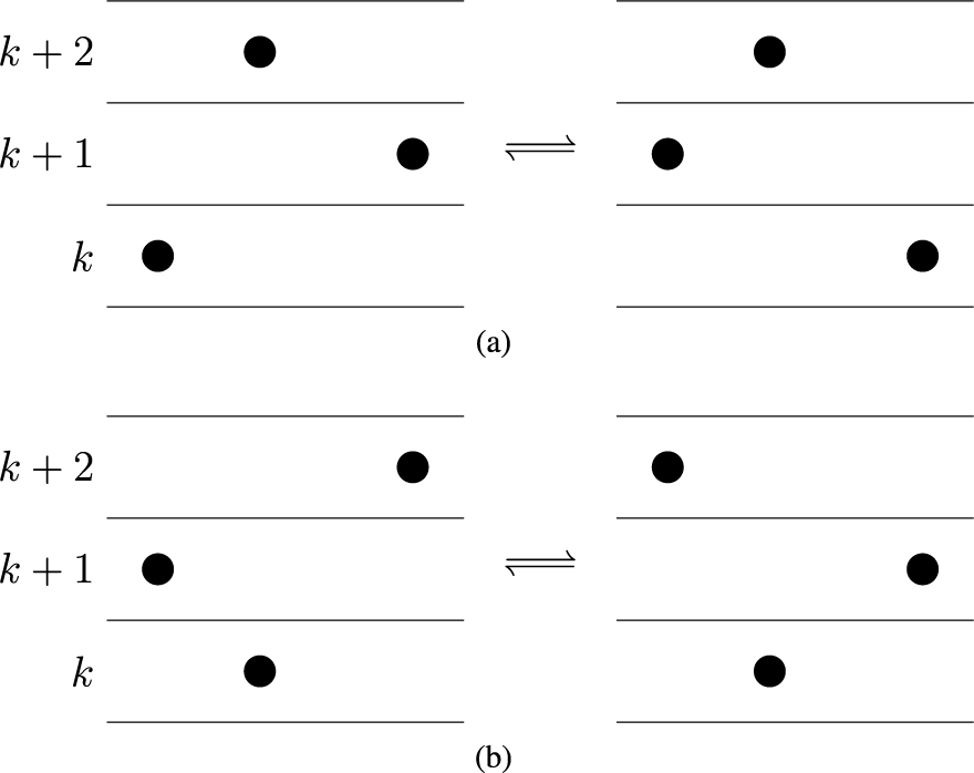
In the following theorem, we report a statement dual to Proposition A.1. We omit the proof, as the arguments are equivalent to those presented immediately above.
Theorem A.16. Consider a pair of weighted permutations $\overline {\pi } \stackrel {*}{\simeq }_{\mathrm {g}} \overline {\pi }'$
. Then for all
$\overline {\pi } \stackrel {*}{\simeq }_{\mathrm {g}} \overline {\pi }'$
. Then for all $t \in \mathbb {Z}$
, we have
$t \in \mathbb {Z}$
, we have $Q_t(\overline {\pi }) = Q_t(\overline {\pi }')$
.
$Q_t(\overline {\pi }) = Q_t(\overline {\pi }')$
.
Theorem A.17. Consider weighted permutations $\overline {\pi },\overline {\pi }'$
such that
$\overline {\pi },\overline {\pi }'$
such that $\overline {\pi } \simeq _{\mathrm {g}} \overline {\pi '}$
or
$\overline {\pi } \simeq _{\mathrm {g}} \overline {\pi '}$
or $\overline {\pi } \stackrel {*}{\simeq }_{\mathrm {g}} \overline {\pi }'$
. Then, for all k, we have
$\overline {\pi } \stackrel {*}{\simeq }_{\mathrm {g}} \overline {\pi }'$
. Then, for all k, we have
 $$ \begin{align} I_k(\overline{\pi}) = I_k(\overline{\pi}') \qquad \text{and} \qquad D_k(\overline{\pi}) = D_k(\overline{\pi}'). \end{align} $$
Proof. Let $(P,Q),(P',Q)'$
be pairs of tableaux such that
$(P,Q),(P',Q)'$
be pairs of tableaux such that $(P,Q)\xrightarrow []{\mathbf {SS}\,} \overline {\pi }$
and
$(P,Q)\xrightarrow []{\mathbf {SS}\,} \overline {\pi }$
and $(P,Q)\xrightarrow []{\mathbf {SS}\,} \overline {\pi }'$
. We have shown in Proposition A.11 that if
$(P,Q)\xrightarrow []{\mathbf {SS}\,} \overline {\pi }'$
. We have shown in Proposition A.11 that if $\overline {\pi } \simeq _{\mathrm {g}} \overline {\pi '}$
, then
$\overline {\pi } \simeq _{\mathrm {g}} \overline {\pi '}$
, then $P_t=P_t^{\prime }$
for all t. In particular, this shows that the asymptotic increment
$P_t=P_t^{\prime }$
for all t. In particular, this shows that the asymptotic increment $\mu $
is common for both pairs
$\mu $
is common for both pairs $(P,Q)$
and
$(P,Q)$
and $(P',Q')$
. By Proposition 6.6, this implies that
$(P',Q')$
. By Proposition 6.6, this implies that $I_k,D_k$
are invariant under generalized Knuth relations. The same statement for dual generalized Knuth relations can be proven analogously.
$I_k,D_k$
are invariant under generalized Knuth relations. The same statement for dual generalized Knuth relations can be proven analogously.
B Proof of Proposition 6.4
We will proceed by direct inspection. Arguments implemented here can be thought of as affine generalizations of those originally presented in [Reference Danilov and Koshevoy23] and [Reference van Leeuwen86]. We organize the proof of Proposition 6.4 in a number of lemmas. The first basic property we prove is that the inversion $\overline {\pi } \to \overline {\pi }^{-1}$
preserves increasing and localized decreasing subsequences.
$\overline {\pi } \to \overline {\pi }^{-1}$
preserves increasing and localized decreasing subsequences.
Lemma B.1. For any $\overline {\pi } \in \overline {\mathbb {A}}_{n,n}$
and any k, we have
$\overline {\pi } \in \overline {\mathbb {A}}_{n,n}$
and any k, we have
 $$ \begin{align} I_k(\overline{\pi}^{-1}) = I_k(\overline{\pi}) \qquad \text{and} \qquad D_k(\overline{\pi}^{-1}) = D_k(\overline{\pi}). \end{align} $$
Proof. We prove that inversion $\overline {\pi } \to \overline {\pi }^{-1}$
, corresponding to the transposition
$\overline {\pi } \to \overline {\pi }^{-1}$
, corresponding to the transposition $\overline {M}_{i,j}(k) \to \overline {M}_{j,i}(k)$
, preserves both increasing and localized increasing subsequences. Let us start with localized decreasing subsequences. A path
$\overline {M}_{i,j}(k) \to \overline {M}_{j,i}(k)$
, preserves both increasing and localized increasing subsequences. Let us start with localized decreasing subsequences. A path $\varsigma =(\varsigma _j: j=1,\dots ,s ) \subset \mathscr {C}_n$
is a strict down-right loop if and only if its points have coordinates
$\varsigma =(\varsigma _j: j=1,\dots ,s ) \subset \mathscr {C}_n$
is a strict down-right loop if and only if its points have coordinates
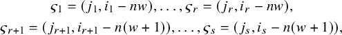 $$ \begin{gather*} \varsigma_1=(j_1,i_1-nw), \dots, \varsigma_r=(j_r,i_r-nw), \\ \varsigma_{r+1}=(j_{r+1},i_{r+1}-n(w+1)), \dots, \varsigma_s=(j_s,i_s-n(w+1)), \end{gather*} $$
for some $r,w$
and numbers
$r,w$
and numbers $i_k,j_k$
such that
$i_k,j_k$
such that
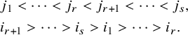 $$ \begin{align} \begin{aligned} &j_1 < \cdots < j_r < j_{r+1} < \cdots < j_s, \\ &i_{r+1} > \cdots > i_s > i_1 > \cdots > i_r. \end{aligned} \end{align} $$
Denote with $\varpi ^T$
the image under transposition
$\varpi ^T$
the image under transposition $(j,i-nw)\to (i,j-nw)$
of the path
$(j,i-nw)\to (i,j-nw)$
of the path $\varpi $
. Then its coordinates are
$\varpi $
. Then its coordinates are
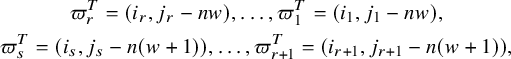 $$ \begin{gather*} \varpi_r^T=(i_r,j_r-nw), \dots, \varpi_1^T=(i_1,j_1-nw), \\ \varpi_s^T=(i_s,j_s-n(w+1)), \dots, \varpi_{r+1}^T=(i_{r+1},j_{r+1}-n(w+1)), \end{gather*} $$
which, by equation (B.2), form again a strict down-right loop.
The proof that transposition maps increasing subsequences $\varpi $
into increasing subsequences
$\varpi $
into increasing subsequences $\varpi ^T$
is also straightforward and therefore we omit it.
$\varpi ^T$
is also straightforward and therefore we omit it.
Lemma B.2. We have $I_k(\iota _{\epsilon }(\overline {\pi })) = I_k(\overline {\pi })$
and
$I_k(\iota _{\epsilon }(\overline {\pi })) = I_k(\overline {\pi })$
and $D_k(\iota _{\epsilon }(\overline {\pi })) = D_k(\overline {\pi })$
for all
$D_k(\iota _{\epsilon }(\overline {\pi })) = D_k(\overline {\pi })$
for all $\overline {\pi }\in \overline {\mathbb {A}}_{n,n}$
,
$\overline {\pi }\in \overline {\mathbb {A}}_{n,n}$
, $\epsilon =1,2$
and
$\epsilon =1,2$
and $k=1,2,\dots $
. Equivalently, recalling the shift
$k=1,2,\dots $
. Equivalently, recalling the shift $T_{\epsilon }$
of equation (5.29),
$T_{\epsilon }$
of equation (5.29), $I_k(T_{\epsilon }(\overline {M})) = I_k(\overline {M})$
and
$I_k(T_{\epsilon }(\overline {M})) = I_k(\overline {M})$
and $D_k(T_{\epsilon }(\overline {M})) = D_k(\overline {M})$
for all
$D_k(T_{\epsilon }(\overline {M})) = D_k(\overline {M})$
for all $\overline {M}\in \overline {\mathbb {M}}_{n\times n}$
,
$\overline {M}\in \overline {\mathbb {M}}_{n\times n}$
, $\epsilon =1,2$
,
$\epsilon =1,2$
, $k=1,2,\dots $
.
$k=1,2,\dots $
.
Proof. This is obvious since shifts $T_1,T_2$
preserve up-right paths and strict down-right loops.
$T_1,T_2$
preserve up-right paths and strict down-right loops.
As a result of Propositions B.1 and B.2 and of definition (5.31), (5.33) of family $\widetilde {E}^{(2)}_i,\widetilde {F}^{(2)}_i$
, in order to prove Proposition 6.4, it suffices to show that
$\widetilde {E}^{(2)}_i,\widetilde {F}^{(2)}_i$
, in order to prove Proposition 6.4, it suffices to show that
 $$ \begin{align} I_k(\widetilde{E}^{(1)}_i(\overline{\pi})) = I_k(\overline{\pi}), \qquad D_k(\widetilde{E}^{(1)}_i(\overline{\pi})) = D_k(\overline{\pi}), \end{align} $$
for all $i=1,\dots ,n-1$
. In the remaining lemmas below, these are indeed the only situations we consider. We start by showing that classical Kashiwara operators preserve increasing subsequences.
$i=1,\dots ,n-1$
. In the remaining lemmas below, these are indeed the only situations we consider. We start by showing that classical Kashiwara operators preserve increasing subsequences.
Lemma B.3. Let $\overline {\pi } \in \overline {\mathbb {A}}_{n,n}$
and
$\overline {\pi } \in \overline {\mathbb {A}}_{n,n}$
and $i\in \{1,\dots ,n-1\}$
such that
$i\in \{1,\dots ,n-1\}$
such that $\widetilde {E}^{(1)}_i(\overline {\pi })$
exists. Then
$\widetilde {E}^{(1)}_i(\overline {\pi })$
exists. Then $I_k(\widetilde {E}^{(1)}_i(\overline {\pi }))=I_k(\overline {\pi })$
.
$I_k(\widetilde {E}^{(1)}_i(\overline {\pi }))=I_k(\overline {\pi })$
.
Proof. Define $\overline {\pi }' = \widetilde {E}^{(1)}_i(\overline {\pi })$
, and let
$\overline {\pi }' = \widetilde {E}^{(1)}_i(\overline {\pi })$
, and let
![]() be a k-increasing subsequence of
be a k-increasing subsequence of $\overline {\pi }$
. We show that we can always find a k-increasing subsequence
$\overline {\pi }$
. We show that we can always find a k-increasing subsequence $\overline {\xi } \subset \overline {\pi }'$
such that
$\overline {\xi } \subset \overline {\pi }'$
such that $|\overline {\xi }| = |\overline {\sigma }|$
, and this clearly implies the claim of the lemma. The weighted biword
$|\overline {\xi }| = |\overline {\sigma }|$
, and this clearly implies the claim of the lemma. The weighted biword $\overline {\pi }'$
is obtained from
$\overline {\pi }'$
is obtained from $\overline {\pi }$
by replacing one entry
$\overline {\pi }$
by replacing one entry $\left ( \begin {smallmatrix} \widehat {j} \\ i+1 \\ \widehat {w} \end {smallmatrix} \right )$
by
$\left ( \begin {smallmatrix} \widehat {j} \\ i+1 \\ \widehat {w} \end {smallmatrix} \right )$
by $\left ( \begin {smallmatrix} \widehat {j} \\ i \\ \widehat {w} \end {smallmatrix} \right )$
, where
$\left ( \begin {smallmatrix} \widehat {j} \\ i \\ \widehat {w} \end {smallmatrix} \right )$
, where $\widehat {j}, \widehat {w}$
are selected through the signature rule (5.25). We denote the corresponding cells
$\widehat {j}, \widehat {w}$
are selected through the signature rule (5.25). We denote the corresponding cells $\widehat {c}=(\widehat {j} - n \widehat {w},i+1)$
and
$\widehat {c}=(\widehat {j} - n \widehat {w},i+1)$
and $\widehat {c}'=\widehat {c} - \mathbf {e}_2$
. In case
$\widehat {c}'=\widehat {c} - \mathbf {e}_2$
. In case $\widehat {c}\notin \overline {\sigma }$
, then
$\widehat {c}\notin \overline {\sigma }$
, then $\overline {\sigma }$
is not affected by transformation
$\overline {\sigma }$
is not affected by transformation $\widetilde {E}^{(1)}_i$
and we simply take
$\widetilde {E}^{(1)}_i$
and we simply take $\overline {\xi } = \overline {\sigma }$
. Alternatively, assume
$\overline {\xi } = \overline {\sigma }$
. Alternatively, assume $\widehat {c} \in \overline {\sigma }$
and without loss of generality let
$\widehat {c} \in \overline {\sigma }$
and without loss of generality let $\widehat {c} \in \overline {\sigma }^{(1)}$
. We write
$\widehat {c} \in \overline {\sigma }^{(1)}$
. We write
 $$ \begin{align} \overline{\sigma}^{(1)} = a_1 \to \cdots \to a_K \to \widehat{c} \to b_1 \to \cdots \to b_J, \end{align} $$
for some increasing subsequences $A=a_1 \to \dots \to a_K$
and
$A=a_1 \to \dots \to a_K$
and $B=b_1 \to \cdots \to b_J$
. In case
$B=b_1 \to \cdots \to b_J$
. In case $A \to \widehat {c}'$
is still an increasing sequence, we define
$A \to \widehat {c}'$
is still an increasing sequence, we define $\overline {\xi }^{(1)} = A \to \widehat {c}' \to B$
and
$\overline {\xi }^{(1)} = A \to \widehat {c}' \to B$
and
![]() is the desired k-increasing subsequence of
is the desired k-increasing subsequence of $\overline {\pi }'$
.
$\overline {\pi }'$
.
The only nontrivial case to treat therefore occurs when $A \to \widehat {c}'$
is no longer an increasing sequence, as in Figure 24. This happens only when point
$A \to \widehat {c}'$
is no longer an increasing sequence, as in Figure 24. This happens only when point $a_S,\dots , a_K$
have coordinates
$a_S,\dots , a_K$
have coordinates $a_s = (j_s, i+1)$
for
$a_s = (j_s, i+1)$
for $s=S,\dots ,K$
. With no loss of generality, we assume that
$s=S,\dots ,K$
. With no loss of generality, we assume that $a_{S-1}$
does not lie on the strip
$a_{S-1}$
does not lie on the strip $\mathbb {Z} \times \{i+1\}$
. By signature rule (5.25), there exists a set of points
$\mathbb {Z} \times \{i+1\}$
. By signature rule (5.25), there exists a set of points $U = \{ u_S, \dots , u_K\}$
with coordinates
$U = \{ u_S, \dots , u_K\}$
with coordinates $u_s = (j_s^{\prime },i)$
such that
$u_s = (j_s^{\prime },i)$
such that $j_s < j_s^{\prime } \le \widehat {j}$
. If
$j_s < j_s^{\prime } \le \widehat {j}$
. If $U \cap \overline {\sigma } = \varnothing $
, we define
$U \cap \overline {\sigma } = \varnothing $
, we define
 $$ \begin{align} \overline{\xi}^{(1)}=a_1 \to \cdots \to a_{S-1} \to u_S \to \cdots \to u_K \to \widehat{c}' \to B \end{align} $$
and again
![]() has the desired properties. This procedure is given in Figure 24, where the solid red path denotes
has the desired properties. This procedure is given in Figure 24, where the solid red path denotes $\overline {\sigma }^{(1)}$
, while the dotted one denotes
$\overline {\sigma }^{(1)}$
, while the dotted one denotes $\overline {\xi }^{(1)}$
.
$\overline {\xi }^{(1)}$
.
An instance of the relabeling procedure of Proposition B.3.
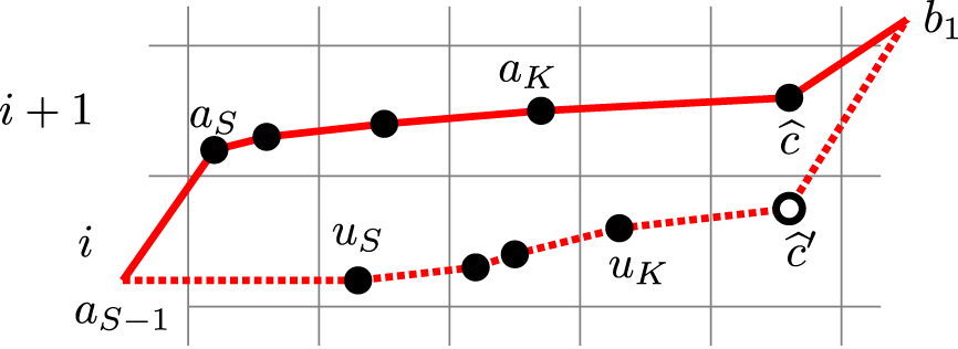
Otherwise, we assume that $U\cap \overline {\sigma } \neq \varnothing $
and let
$U\cap \overline {\sigma } \neq \varnothing $
and let
 $$ \begin{align} J= \max \{s \in \{S,\dots,K\} : u_s \in \overline{\sigma} \}. \end{align} $$
With no loss of generality, we can write
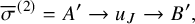 $$ \begin{align} \overline{\sigma}^{(2)} = A' \to u_J \to B', \end{align} $$
for two increasing subsequences $A',B'$
. This situation is reported in panels (a) and (c) of Figure 25, depending on if
$A',B'$
. This situation is reported in panels (a) and (c) of Figure 25, depending on if $\widehat {c}' \to B'$
is increasing or not. There red and blue lines denote
$\widehat {c}' \to B'$
is increasing or not. There red and blue lines denote $\overline {\sigma }^{(1)}$
and
$\overline {\sigma }^{(1)}$
and $\overline {\sigma }^{(2)}$
. When
$\overline {\sigma }^{(2)}$
. When $\widehat {c}' \to B'$
is increasing we set, as in Figure 25 panel (b)
$\widehat {c}' \to B'$
is increasing we set, as in Figure 25 panel (b)
 $$ \begin{align} \overline{\xi}^{(1)} = A \to B, \qquad \overline{\xi}^{(2)} = A' \to u_J \to \widehat{c}' \to B' \end{align} $$
and
![]() is the k-increasing subsequence of
is the k-increasing subsequence of $\overline {\pi }$
we are looking for.
$\overline {\pi }$
we are looking for.
Some of the possible relabeling procedures described in the proof of Proposition B.3.
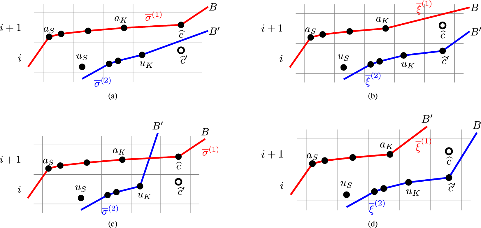
Otherwise, if $\widehat {c}' \to B'$
is not increasing, we define
$\widehat {c}' \to B'$
is not increasing, we define
 $$ \begin{align} \overline{\xi}^{(1)} = a_1 \to \cdots \to a_J \to B', \qquad \overline{\xi}^{(2)} = A' \to u_J \to u_{J+1} \to \cdots \to u_S \to \widehat{c}' \to B, \end{align} $$
as in Figure 25 panels (c) and (d). Also, in this case
![]() has the desired properties. This check exhausts all possibilities and concludes the proof.
has the desired properties. This check exhausts all possibilities and concludes the proof.
The proof of the fact that Kashiwara operators preserve the length of the longest localized decreasing subsequences is slightly more involved than the preservation property for increasing subsequences. We articulate the analysis of this case in the following three lemmas. For the next statement, we need to recall how the shadow line construction one draws for the transition $\overline {\pi } \mapsto \mathbf {V}(\overline {\pi })$
defines an ensemble of down-right loops; see Section 4.3.
$\overline {\pi } \mapsto \mathbf {V}(\overline {\pi })$
defines an ensemble of down-right loops; see Section 4.3.
Lemma B.4. Let $\overline {\pi }$
be a k-localized decreasing sequence. Then the shadow line construction of
$\overline {\pi }$
be a k-localized decreasing sequence. Then the shadow line construction of $\overline {\pi }$
consists of at most k down-right loops.
$\overline {\pi }$
consists of at most k down-right loops.
Proof. We show that if the shadow line construction of $\overline {\pi }$
consists of
$\overline {\pi }$
consists of $\widetilde {k}$
down-right loops
$\widetilde {k}$
down-right loops $\varsigma ^{(1)},\dots ,\varsigma ^{(\widetilde {k})}$
, then there exists an increasing subsequence
$\varsigma ^{(1)},\dots ,\varsigma ^{(\widetilde {k})}$
, then there exists an increasing subsequence $\overline {\xi }\subset \overline {\pi }$
of length
$\overline {\xi }\subset \overline {\pi }$
of length $\widetilde {k}$
. With this assumption, let
$\widetilde {k}$
. With this assumption, let $\overline {\xi } = c_1\to \cdots \to c_{\widetilde {k}}$
be contained in an up-right path in
$\overline {\xi } = c_1\to \cdots \to c_{\widetilde {k}}$
be contained in an up-right path in $\mathscr {C}_n$
. Writing
$\mathscr {C}_n$
. Writing
![]() , where
, where $\overline {\sigma }^{(j)}$
’s are localized decreasing subsequences, no two
$\overline {\sigma }^{(j)}$
’s are localized decreasing subsequences, no two $c_i$
can belong to the same
$c_i$
can belong to the same $\overline {\sigma }^{(j)}$
forcing
$\overline {\sigma }^{(j)}$
forcing $k \ge \widetilde {k}$
.
$k \ge \widetilde {k}$
.
Representing $\mathscr {C}_n$
as an infinite vertical strip, we assume that loops are ordered from the topmost
$\mathscr {C}_n$
as an infinite vertical strip, we assume that loops are ordered from the topmost $\varsigma ^{(1)}$
to the bottom-most
$\varsigma ^{(1)}$
to the bottom-most $\varsigma ^{(\widetilde {k})}$
; see Figure 26. We are left to show that an increasing subsequence of length
$\varsigma ^{(\widetilde {k})}$
; see Figure 26. We are left to show that an increasing subsequence of length $\widetilde {k}$
always exists. For this, we show that if
$\widetilde {k}$
always exists. For this, we show that if $c_i \in \overline {\pi } \cap \varsigma ^{(i)}$
is a point of the configuration lying on the i-th loop of the shadow line construction, then we can always find
$c_i \in \overline {\pi } \cap \varsigma ^{(i)}$
is a point of the configuration lying on the i-th loop of the shadow line construction, then we can always find $c_{i+1} \in \overline {\pi } \cap \varsigma ^{(i+1)}$
such that
$c_{i+1} \in \overline {\pi } \cap \varsigma ^{(i+1)}$
such that $c_{i+1} \to c_{i}$
is an increasing sequence. To find such
$c_{i+1} \to c_{i}$
is an increasing sequence. To find such $c_{i+1}$
, start walking southward from
$c_{i+1}$
, start walking southward from $c_i=(a,b-nw)$
until the first intersection with an horizontal segment of the loop
$c_i=(a,b-nw)$
until the first intersection with an horizontal segment of the loop $\varsigma ^{(i+1)}$
, which happens at a location
$\varsigma ^{(i+1)}$
, which happens at a location $(a,b'-nw')$
for some
$(a,b'-nw')$
for some $b'-nw' \le b-nw$
. From there, travel eastward along
$b'-nw' \le b-nw$
. From there, travel eastward along $\varsigma ^{(i+1)}$
until the first occurrence of a point in
$\varsigma ^{(i+1)}$
until the first occurrence of a point in $c_{i+1} \in \overline {\pi }$
, which might happen after winding around the cylinder. In Figure 26 (b), we represented such walks with red dotted segments. By construction,
$c_{i+1} \in \overline {\pi }$
, which might happen after winding around the cylinder. In Figure 26 (b), we represented such walks with red dotted segments. By construction, $c_{i+1}\to c_i$
forms an increasing sequence and by induction we conclude the proof.
$c_{i+1}\to c_i$
forms an increasing sequence and by induction we conclude the proof.
An example of the construction presented in the proof of Proposition B.4. In the left panel, we see the weighted biword $\overline {\pi }$
represented as an union of four LDSs. In the right panel, we see that the shadow line construction produces three down-right loops.
$\overline {\pi }$
represented as an union of four LDSs. In the right panel, we see that the shadow line construction produces three down-right loops.
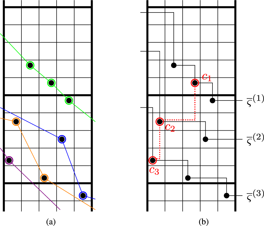
Lemma B.5. Consider a 2-localized decreasing sequence
![]() , and assume
, and assume $\overline {\pi }'=\widetilde {E}^{(1)}_i(\overline {\pi }) \neq \varnothing $
for some
$\overline {\pi }'=\widetilde {E}^{(1)}_i(\overline {\pi }) \neq \varnothing $
for some $i\in \{1,\dots ,n-1\}$
. Then we also have
$i\in \{1,\dots ,n-1\}$
. Then we also have
![]() , for two localized decreasing subsequences
, for two localized decreasing subsequences $\overline {\xi }^{(1)}, \overline {\xi }^{(2)}$
.
$\overline {\xi }^{(1)}, \overline {\xi }^{(2)}$
.
Proof. The weighted biword $\overline {\pi }'$
is obtained from
$\overline {\pi }'$
is obtained from $\overline {\pi }$
replacing an entry
$\overline {\pi }$
replacing an entry $\left ( \begin {smallmatrix} \widehat {j} \\ i+1 \\ \widehat {w} \end {smallmatrix} \right )$
with
$\left ( \begin {smallmatrix} \widehat {j} \\ i+1 \\ \widehat {w} \end {smallmatrix} \right )$
with $\left ( \begin {smallmatrix} \widehat {j} \\ i \\ \widehat {w} \end {smallmatrix} \right )$
, where
$\left ( \begin {smallmatrix} \widehat {j} \\ i \\ \widehat {w} \end {smallmatrix} \right )$
, where $\widehat {j},\widehat {w}$
are selected through the signature rule (5.25), (5.26). Call
$\widehat {j},\widehat {w}$
are selected through the signature rule (5.25), (5.26). Call $\widehat {c}=(\widehat {j}, i+1 - \widehat {w} n)$
and
$\widehat {c}=(\widehat {j}, i+1 - \widehat {w} n)$
and $\widehat {c}' = \widehat {c} - \mathbf {e}_2$
. With no loss of generality, assume
$\widehat {c}' = \widehat {c} - \mathbf {e}_2$
. With no loss of generality, assume $\widehat {c} \in \overline {\sigma }^{(1)}$
and write
$\widehat {c} \in \overline {\sigma }^{(1)}$
and write
 $$ \begin{align} \overline{\sigma}^{(1)} = a_1 \to \cdots \to a_M \qquad \overline{\sigma}^{(2)}= b_1 \to \cdots \to b_N, \end{align} $$
with $\widehat {c}=a_K$
for some K. Representing
$\widehat {c}=a_K$
for some K. Representing $\mathscr {C}_n$
as an infinite vertical strip, we assume cells
$\mathscr {C}_n$
as an infinite vertical strip, we assume cells $a_k,b_k$
to be ordered from top to bottom. Define
$a_k,b_k$
to be ordered from top to bottom. Define
 $$ \begin{align} \overline{\theta} = a_1 \to \dots \to a_{K-1} \to \widehat{c}' \to a_{K+1} \to \dots \to a_M. \end{align} $$
If $\overline {\theta }$
is an LDS, we set
$\overline {\theta }$
is an LDS, we set $\overline {\xi }^{(1)}=\overline {\theta }$
and
$\overline {\xi }^{(1)}=\overline {\theta }$
and $\overline {\xi }^{(2)}=\overline {\sigma }^{(2)}$
and this yields the desired decomposition of
$\overline {\xi }^{(2)}=\overline {\sigma }^{(2)}$
and this yields the desired decomposition of $\overline {\pi }'$
. To check the remaining cases, we consider two possibilities.
$\overline {\pi }'$
. To check the remaining cases, we consider two possibilities.
Case 1: $\overline {\theta }$
is not localized. This only happens if
$\overline {\theta }$
is not localized. This only happens if $\widehat {c}=a_M$
and
$\widehat {c}=a_M$
and $a_1=(j_1,i-n(\widehat {w}-1))$
, for some
$a_1=(j_1,i-n(\widehat {w}-1))$
, for some $1\le j_1 < \widehat {j}$
. From the signature rule (5.26), this implies that there exists a point
$1\le j_1 < \widehat {j}$
. From the signature rule (5.26), this implies that there exists a point $\widehat {d} \in \overline {\sigma }^{(2)}$
such that
$\widehat {d} \in \overline {\sigma }^{(2)}$
such that $\widehat {d}=(j_2, i+1 - n (\widehat {w}-1))$
, with
$\widehat {d}=(j_2, i+1 - n (\widehat {w}-1))$
, with $1 \le j_2 < j_1$
, or
$1 \le j_2 < j_1$
, or $\widehat {d} = (\tilde {j}_2,i+1- n \widehat {w})$
with
$\widehat {d} = (\tilde {j}_2,i+1- n \widehat {w})$
with $\widehat {j}<\tilde {j}_2 \le n$
. We treat these two additional subcases separately.
$\widehat {j}<\tilde {j}_2 \le n$
. We treat these two additional subcases separately.
-
Case 1.1:
$\widehat {d}=(j_2, i+1 - n (\widehat {w}-1))$
. We can write subsequence
$\overline {\sigma }^{(2)} = U \to V$
, where
$U=u_1 \to \cdots \to u_J$
is the LDS of all
$u_j \in \overline {\sigma }^{(2)}$
such that
$u_j \to a_1$
is an LDS; see Figure 27 (a) for an example. Notice that
$u_J=\widehat {d}$
. Define sector
$S=\{ 1,\dots ,n \} \times \{ i+1 - n \widehat {w} , \dots , i-1 - n (\widehat {w}-1) \}$
as in Figure 27 (b). By construction, S contains all points of
$\overline {\pi }$
except for U and
$a_1$
. Moreover, all points in S are contained in two LDS: V and
$a_2 \to \cdots \to a_M$
. We draw the shadow line construction, restricted to the sector S, of all points contained in S, as in Figure 27 (b). By an adaptation of Proposition B.4, such shadow line construction consists of at most two down-right broken lines we call
$\overline {\varsigma }^{(1)}, \overline {\varsigma }^{(2)}$
. With no loss of generality, we assume that
$\widehat {c}\in \overline {\varsigma }^{(1)}$
and this forces
$\overline {\varsigma }^{(2)}$
to contain only points of
$\overline {\pi }$
that are weakly to east of
$a_2$
and weakly north of
$b_N$
. Define now
$W^{(2)}$
selecting all points of
$\overline {\pi } \cap \overline {\varsigma }^{(2)}$
, without multiplicity and
$\overline {\xi }^{(2)} = U \to a_1 \to \sigma ^{(2)}$
. Then
$\overline {\xi }^{(2)}$
is an LDS. Subsequently, define
$W^{(1)}$
taking all points of
$\overline {\pi } \cap \overline {\varsigma }^{(1)}$
minus
$\widehat {c}$
, and set
$\overline {\xi }^{(1)} = W^{(1)} \to \widehat {c}'$
. Again
$\overline {\xi }^{(1)}$
is an LDS and
$\overline {\xi }^{(1)}, \overline {\xi }^{(2)}$
provide the desired decomposition of
$\overline {\pi }'$
Figure 27Relabeling procedure corresponding to Case 1.1 in the proof of Proposition B.5. Red and blue LDSs in the left panel are
$\overline {\sigma }^{(1)},\overline {\sigma }^{(2)}$
. In the right panel, red and blue LDSs are
$\overline {\xi }^{(1)},\overline {\xi }^{(2)}$
.Figure 28Relabeling procedure corresponding to Case 1.2 in proof of Proposition B.5. In the left panel, red and blue LDSs are
$\overline {\sigma }^{(1)}, \overline {\sigma }^{(2)}$
, while in the right panel they are
$\overline {\xi }^{(1)}, \overline {\xi }^{(2)}$
. -
Case 1.2:
$\widehat {d}=(\tilde {j}_2, i+1 - n \widehat {w})$
. This case is represented in Figure 28 (a). We write
$\overline {\sigma }^{(2)} = U \to V$
, with U having all points located weakly north of
$\widehat {c}$
and V having all points located southeast of
$\widehat {c}'$
. In this case, consider the sector
$S = \{1,\dots , n\}\times \{ i+1-n\widehat {w}, \dots , i - n (\widehat {w}-1) \}$
as in Figure 28 (b). Then all points of
$\overline {\pi }$
except those in V are contained in S. By the signature rule,
$a_1$
is the northernmost point of the configuration as no other point can be of the form
$(j,i-n(\widehat {w}-1))$
. Moreover, points in S all belong to the union of down-right paths U and
$\overline {\sigma }^{(1)}$
. Therefore, the inverse shadow line construction, restricted to the sector S, of the points within S, drawn in Figure 28 (b), will consist, again by an adaptation of Proposition B.4, of exactly two separate broken lines
$\overline {\varsigma }^{(1)},\overline {\varsigma }^{(2)}$
. With no loss of generality, we assume that
$\widehat {c} \in \overline {\varsigma }^{(1)}$
, while
$\widehat {d},a_1 \in \overline {\varsigma }^{(2)}$
, which implies that
$\overline {\varsigma }^{(1)}$
is contained in the region weakly south of
$b_1$
. We now define LDS
$\overline {\xi }^{(2)}$
taking points
$\overline {\pi } \cap \overline {\varsigma }^{(2)}$
without multiplicity. Define also W taking points
$\overline {\pi } \cap \overline {\varsigma }^{(1)}$
, without mulitplicity and excluding
$\widehat {c}$
. Finally, we set
$\overline {\xi }^{(1)}=W \to \widehat {c}' \to V$
. Also, in this case the decomposition
has the desired properties.Figure 29Depiction of the relabeling described in Case 2 in the proof of Proposition B.5.


Case 2: $\overline {\theta }$
is not strictly down right. This can only happen if
$\overline {\theta }$
is not strictly down right. This can only happen if $\widehat {c}=a_K$
and
$\widehat {c}=a_K$
and $a_{K+1}=(j_1, i-n\widehat {w})$
for some
$a_{K+1}=(j_1, i-n\widehat {w})$
for some $j_1\in \{ \widehat {j}+1,\cdots ,n \}$
and some K. See Figure 29 (a) for an example. By the signature rule, there must exist
$j_1\in \{ \widehat {j}+1,\cdots ,n \}$
and some K. See Figure 29 (a) for an example. By the signature rule, there must exist $\widehat {d}\in \overline {\sigma }^{(2)}$
such that
$\widehat {d}\in \overline {\sigma }^{(2)}$
such that $\widehat {d}=(j_2,i+1-n\widehat {w})$
with
$\widehat {d}=(j_2,i+1-n\widehat {w})$
with $j_2 \in \{\widehat {j},\cdots j_1-1\}$
and moreover no other point occupies the segment of vertical coordinate
$j_2 \in \{\widehat {j},\cdots j_1-1\}$
and moreover no other point occupies the segment of vertical coordinate $i - n \widehat {w}$
. We draw the inverse shadow line construction of the point configuration, which consists in two down-right paths
$i - n \widehat {w}$
. We draw the inverse shadow line construction of the point configuration, which consists in two down-right paths $\overline {\varsigma }^{(1)}, \overline {\varsigma }^{(2)}$
, by Proposition B.4. Because of their relative position, we must have,
$\overline {\varsigma }^{(1)}, \overline {\varsigma }^{(2)}$
, by Proposition B.4. Because of their relative position, we must have, $a_K \in \overline {\varsigma }^{(1)}$
, while
$a_K \in \overline {\varsigma }^{(1)}$
, while $a_{K+1}, \widehat {d} \in \overline {\varsigma }^{(2)}$
. Then we define
$a_{K+1}, \widehat {d} \in \overline {\varsigma }^{(2)}$
. Then we define $\overline {\xi }^{(1)}$
taking points in
$\overline {\xi }^{(1)}$
taking points in $\overline {\pi } \cap \overline {\varsigma }^{(1)}$
, without multiplicity, and replacing
$\overline {\pi } \cap \overline {\varsigma }^{(1)}$
, without multiplicity, and replacing $\widehat {c}$
by
$\widehat {c}$
by $\widehat {c}'$
; see Figure 29 (b). Define also
$\widehat {c}'$
; see Figure 29 (b). Define also $\overline {\xi }^{(2)}$
taking point in
$\overline {\xi }^{(2)}$
taking point in $\overline {\pi } \cap \overline {\varsigma }^{(2)}$
. Both
$\overline {\pi } \cap \overline {\varsigma }^{(2)}$
. Both $\overline {\xi }^{(1)}, \overline {\xi }^{(2)}$
are LDSs, and their union is
$\overline {\xi }^{(1)}, \overline {\xi }^{(2)}$
are LDSs, and their union is $\overline {\pi }'$
. The analysis of this case exhausts all possible configurations of
$\overline {\pi }'$
. The analysis of this case exhausts all possible configurations of $\overline {\sigma }^{(1)}, \overline {\sigma }^{(2)}$
and completes the proof.
$\overline {\sigma }^{(1)}, \overline {\sigma }^{(2)}$
and completes the proof.
Lemma B.6. Let $\overline {\pi } \in \overline {\mathbb {A}}_{n,n}$
and
$\overline {\pi } \in \overline {\mathbb {A}}_{n,n}$
and $\overline {\pi }'=\widetilde {E}^{(1)}_i (\overline {\pi }) \neq \varnothing $
for some
$\overline {\pi }'=\widetilde {E}^{(1)}_i (\overline {\pi }) \neq \varnothing $
for some $i\in \{1,\dots ,n-1\}$
. Then, for all k, we have
$i\in \{1,\dots ,n-1\}$
. Then, for all k, we have $D_k(\overline {\pi }')=D_k(\overline {\pi })$
.
$D_k(\overline {\pi }')=D_k(\overline {\pi })$
.
Proof. As discussed several times above, $\overline {\pi }'$
differs from
$\overline {\pi }'$
differs from $\overline {\pi }$
by a replacement of
$\overline {\pi }$
by a replacement of $\left ( \begin {smallmatrix} \widehat {j} \\ i+1 \\ \widehat {w} \end {smallmatrix} \right )$
with
$\left ( \begin {smallmatrix} \widehat {j} \\ i+1 \\ \widehat {w} \end {smallmatrix} \right )$
with $\left ( \begin {smallmatrix} \widehat {j} \\ i \\ \widehat {w} \end {smallmatrix} \right )$
. For this proof, it is convenient to parameterize
$\left ( \begin {smallmatrix} \widehat {j} \\ i \\ \widehat {w} \end {smallmatrix} \right )$
. For this proof, it is convenient to parameterize $\mathscr {C}_n$
as the infinite horizontal strip (4.4) and we define points
$\mathscr {C}_n$
as the infinite horizontal strip (4.4) and we define points $\widehat {c}=(\widehat {j}+ \widehat {w} n, i+1)$
and
$\widehat {c}=(\widehat {j}+ \widehat {w} n, i+1)$
and $\widehat {c}' = \widehat {c}-\mathbf {e}_2$
. Let
$\widehat {c}' = \widehat {c}-\mathbf {e}_2$
. Let
![]() be a k-LDS of
be a k-LDS of $\overline {\pi }$
. We show that we can find a k-LDS
$\overline {\pi }$
. We show that we can find a k-LDS
![]() with the same length of
with the same length of $\overline {\sigma }$
and this statement clearly implies the result of the lemma.
$\overline {\sigma }$
and this statement clearly implies the result of the lemma.
Clearly, if $\widehat {c}\notin \overline {\sigma }$
we take
$\widehat {c}\notin \overline {\sigma }$
we take $\overline {\xi } = \overline {\sigma }$
and there is nothing to prove. We then assume, with no loss of generality that
$\overline {\xi } = \overline {\sigma }$
and there is nothing to prove. We then assume, with no loss of generality that $\widehat {c} \in \overline {\sigma }^{(1)}$
and in particular
$\widehat {c} \in \overline {\sigma }^{(1)}$
and in particular $\widehat {c}=[\overline {\sigma }^{(1)}_K]$
for some K. As in the proof of Proposition B.5, define
$\widehat {c}=[\overline {\sigma }^{(1)}_K]$
for some K. As in the proof of Proposition B.5, define
 $$ \begin{align} \overline{\theta} = [\overline{\sigma}^{(1)}_1] \to \cdots \to [\overline{\sigma}^{(1)}_{K-1}] \to \widehat{c}' \to [\overline{\sigma}^{(1)}_{K+1}] \to \cdots. \end{align} $$
If $\overline {\theta }$
is an LDS, then we set
$\overline {\theta }$
is an LDS, then we set
![]() , producing the desired k-LDS
, producing the desired k-LDS $\overline {\xi } \subseteq \overline {\pi }'$
. If, on the other hand,
$\overline {\xi } \subseteq \overline {\pi }'$
. If, on the other hand, $\overline {\theta }$
is not an LDS, then there exists
$\overline {\theta }$
is not an LDS, then there exists $\widetilde {c} \in \overline {\sigma }^{(1)}$
such that
$\widetilde {c} \in \overline {\sigma }^{(1)}$
such that $\widetilde {c}=(\widetilde {j},i)$
for some
$\widetilde {c}=(\widetilde {j},i)$
for some $\widehat {j} < \widetilde {j}$
. Define
$\widehat {j} < \widetilde {j}$
. Define $\Omega ^{(i)}(\overline {\pi }; \overline {\sigma })$
as the set of
$\Omega ^{(i)}(\overline {\pi }; \overline {\sigma })$
as the set of $a = (m,i+1) \in \overline {\pi }$
such that
$a = (m,i+1) \in \overline {\pi }$
such that
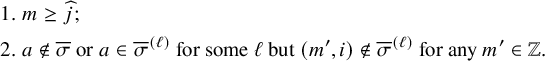 $$ \begin{align} \begin{aligned}&1.\ m \ge \widehat{j};\\&2.\ a \notin \overline{\sigma} \text{ or } a \in \overline{\sigma}^{(\ell)} \text{ for some } \ell \text{ but } (m',i)\notin \overline{\sigma}^{(\ell)} \text{ for any } m' \in \mathbb{Z}. \qquad\qquad\qquad\qquad\qquad\end{aligned} \end{align} $$
Then, by the signature rule $\Omega ^{(i)}(\overline {\pi }; \overline {\sigma })$
is not empty and we consider its element
$\Omega ^{(i)}(\overline {\pi }; \overline {\sigma })$
is not empty and we consider its element $\widehat {d}=(\widehat {m},i+1)$
situated furthest to the west. By this, we mean that
$\widehat {d}=(\widehat {m},i+1)$
situated furthest to the west. By this, we mean that $(m,i+1)\notin \Omega ^{(i)}(\overline {\pi }; \overline {\sigma })$
for any
$(m,i+1)\notin \Omega ^{(i)}(\overline {\pi }; \overline {\sigma })$
for any $m < \widehat {m}$
. Based on the position of
$m < \widehat {m}$
. Based on the position of $\widehat {d}$
, we distinguish two cases.
$\widehat {d}$
, we distinguish two cases.
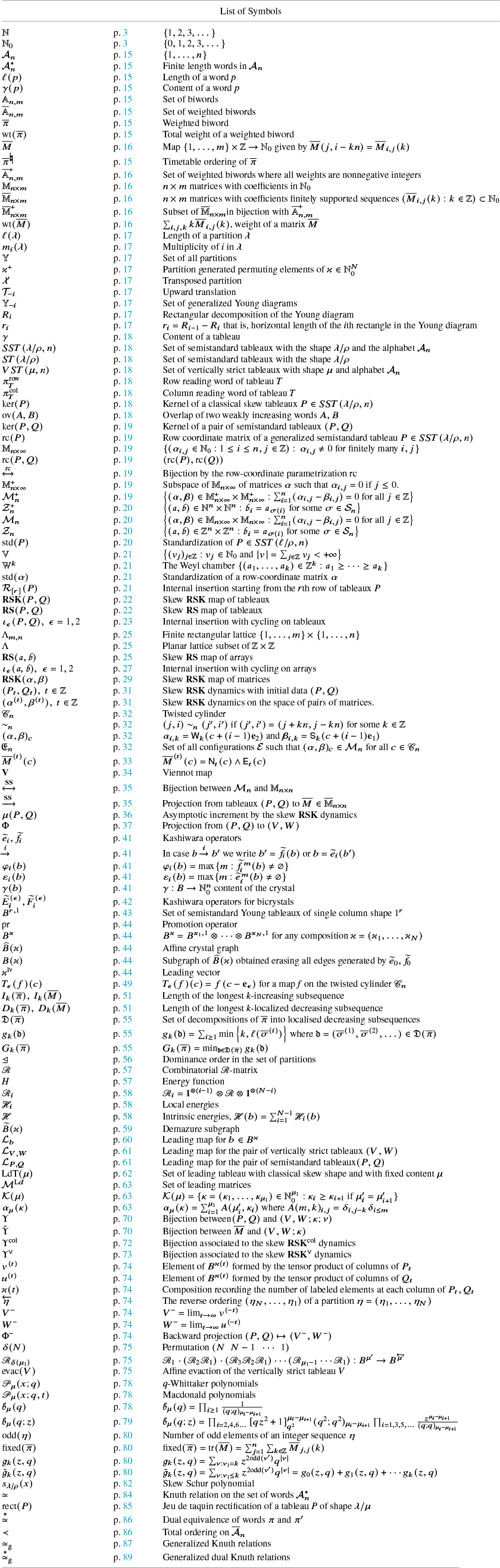
Case 1: $\widehat {d}$
lies between
$\widehat {d}$
lies between $\widehat {c}$
and
$\widehat {c}$
and $\widetilde {c}$
. More precisely, we assume
$\widetilde {c}$
. More precisely, we assume $\widehat {j}\le \widehat {m} < \widetilde {j}$
. Then:
$\widehat {j}\le \widehat {m} < \widetilde {j}$
. Then:
-
• if
$\widehat {d}\notin \overline {\sigma }$
, we can define
$\overline { \xi }^{(1)}$
replacing, in
$\overline {\sigma }^{(1)}$
,
$\widehat {c}$
with
$\widehat {d}$
. This produces the desires k-LDS
. -
• if
$\widehat {d} \in \overline {\sigma }$
and with no loss of generality, we assume
$\widehat {d} \in \overline {\sigma }^{(2)}$
, then weighted biword
satisfies the hypothesis of Proposition B.5. By the same lemma, we can find a decomposition
and
yields the desired k-LDS of
$\overline {\pi }'$
. This situation is reported in Figure 30.Figure 30An example of configuration where
$\widehat {d} \in \overline {\sigma }^{(2)}$
lies between
$\widehat {c}$
and
$\widetilde {c}$
.Figure 31An example of a configuration where
$\widehat {d}$
does not lie between
$\widehat {c}$
and
$\widetilde {c}$
.


Case 2: $\widehat {d}$
does not lie between
$\widehat {d}$
does not lie between $\widehat {c}$
and
$\widehat {c}$
and $\widetilde {c}$
. When
$\widetilde {c}$
. When $\widehat {m}\ge \widetilde {j}$
, we want to show that through a series of reshuffling of elements of
$\widehat {m}\ge \widetilde {j}$
, we want to show that through a series of reshuffling of elements of $\overline {\sigma }$
and
$\overline {\sigma }$
and $\overline {\pi }$
we can always ‘transport’ the point
$\overline {\pi }$
we can always ‘transport’ the point $\widehat {d}$
in the region between
$\widehat {d}$
in the region between $\widehat {c}$
and
$\widehat {c}$
and $\widetilde {c}$
, falling back into Case 1. By the signature rule and by definition of
$\widetilde {c}$
, falling back into Case 1. By the signature rule and by definition of $\widehat {d}$
, it is easy to conclude that there exist points
$\widehat {d}$
, it is easy to conclude that there exist points $a=(j_a,i+1)$
,
$a=(j_a,i+1)$
, $b=(j_b,i)$
such that
$b=(j_b,i)$
such that
 $$ \begin{align} \begin{aligned}&1. \ a,b \in \overline{\sigma}^{(s)} \text{ for some } s.\\&2. \ a \text{ lies between } \widehat{c} \text{ and } \widehat{d}, \text{ while } b \text{ lies to east of } \widehat{d}. \text{ More precisely, } \widehat{j} \le j_a < \widehat{m} < j_b.\end{aligned} \end{align} $$
For an example, see Figure 31. In case $\widehat {d} \notin \overline {\sigma }$
, we replace in
$\widehat {d} \notin \overline {\sigma }$
, we replace in $\overline {\sigma }^{(s)}$
, a with
$\overline {\sigma }^{(s)}$
, a with $\widehat {d}$
yielding a new LDS
$\widehat {d}$
yielding a new LDS $\widetilde {\sigma }^{(s)}$
and therefore a new k-LDS
$\widetilde {\sigma }^{(s)}$
and therefore a new k-LDS $\widetilde {\sigma }$
obtained from
$\widetilde {\sigma }$
obtained from $\overline {\sigma }$
interchanging
$\overline {\sigma }$
interchanging $\widetilde {\sigma }^{(s)}$
and
$\widetilde {\sigma }^{(s)}$
and $\overline {\sigma }^{(s)}$
. After such replacement, the set
$\overline {\sigma }^{(s)}$
. After such replacement, the set $\Omega ^{(i)}(\overline {\pi }, \widetilde {\sigma })$
differs from
$\Omega ^{(i)}(\overline {\pi }, \widetilde {\sigma })$
differs from $\Omega ^{(i)}(\overline {\pi }, \overline {\sigma })$
and, in particular, its westernmost element is a, rather than
$\Omega ^{(i)}(\overline {\pi }, \overline {\sigma })$
and, in particular, its westernmost element is a, rather than $\widehat {d}$
. Alternatively, assume
$\widehat {d}$
. Alternatively, assume $\widehat {d}\in \overline {\sigma }$
, say
$\widehat {d}\in \overline {\sigma }$
, say $\widehat {d} \in \overline {\sigma }^{(s+1)}$
for some s. Then as in Case 1 weighted biword
$\widehat {d} \in \overline {\sigma }^{(s+1)}$
for some s. Then as in Case 1 weighted biword
![]() fulfills the hypothesis of Proposition B.5. This implies that we can find a decomposition
fulfills the hypothesis of Proposition B.5. This implies that we can find a decomposition
![]() such that, if
such that, if $a \in \overline {\eta }^{(s)}$
, then
$a \in \overline {\eta }^{(s)}$
, then $(m,i)\notin \overline {\eta }^{(s)}$
for any
$(m,i)\notin \overline {\eta }^{(s)}$
for any $m \in \mathbb {Z}$
. Define now
$m \in \mathbb {Z}$
. Define now $\widetilde {\sigma }$
replacing in
$\widetilde {\sigma }$
replacing in $\overline {\sigma }$
LDSs
$\overline {\sigma }$
LDSs $\overline {\sigma }^{(s)}, \overline {\sigma }^{(s+1)}$
with
$\overline {\sigma }^{(s)}, \overline {\sigma }^{(s+1)}$
with $\overline {\eta }^{(s)}, \overline {\eta }^{(s+1)}$
. Then also in this case the westernmost element of the set
$\overline {\eta }^{(s)}, \overline {\eta }^{(s+1)}$
. Then also in this case the westernmost element of the set $\Omega ^{(i)}(\overline {\pi },\widetilde {\sigma })$
is no longer
$\Omega ^{(i)}(\overline {\pi },\widetilde {\sigma })$
is no longer $\widehat {d}$
, but a. This shows that, inductively, we can move west, through reshuffling, the westernmost element of
$\widehat {d}$
, but a. This shows that, inductively, we can move west, through reshuffling, the westernmost element of $\Omega ^{(i)}(\overline {\pi },\overline {\sigma })$
until it lies between
$\Omega ^{(i)}(\overline {\pi },\overline {\sigma })$
until it lies between $\widehat {c}$
and
$\widehat {c}$
and $\widetilde {c}$
, which is then treated by Case 1. This concludes the proof.
$\widetilde {c}$
, which is then treated by Case 1. This concludes the proof.
We finally arrive at the proof of Proposition 6.4.
Proof of Proposition 6.4.
It follows by combining the results of the lemmas enumerated in this appendix. Thanks to Proposition B.1, the family of Kashiwara operators $\widetilde {E}^{(2)}_i,\widetilde {F}^{(2)}_i$
preserves the quantities
$\widetilde {E}^{(2)}_i,\widetilde {F}^{(2)}_i$
preserves the quantities $I_k,D_k$
only if the first family
$I_k,D_k$
only if the first family $\widetilde {E}^{(1)}_i,\widetilde {F}^{(1)}_i$
does. Furthermore, through Proposition B.2 one simply has to check that
$\widetilde {E}^{(1)}_i,\widetilde {F}^{(1)}_i$
does. Furthermore, through Proposition B.2 one simply has to check that $\widetilde {E}^{(1)}_i,\widetilde {F}^{(1)}_i$
preserve
$\widetilde {E}^{(1)}_i,\widetilde {F}^{(1)}_i$
preserve $I_k,D_k$
for
$I_k,D_k$
for $i=1,\dots ,n-1$
. The last case is handled by Proposition B.3 and Proposition B.6. Notice that if
$i=1,\dots ,n-1$
. The last case is handled by Proposition B.3 and Proposition B.6. Notice that if $\widetilde {E}^{(1)}_i$
preserves
$\widetilde {E}^{(1)}_i$
preserves $I_k,D_k$
, then also
$I_k,D_k$
, then also $\widetilde {F}^{(1)}_i$
does, being its inverse.
$\widetilde {F}^{(1)}_i$
does, being its inverse.
Acknowledgments
We thank Nikolaos Zygouras and Kirone Mallick for comments and suggestions on an early version of this paper. We are grateful to Shinji Koshida and Ryosuke Sato for discussions and remarks about representation theoretic aspects of this paper. We also thank Rei Inoue for useful remarks about theory of crystals and integrable systems. MM is grateful to Takato Yoshimura for showing interest in this work and to Alexander Garbali for discussions about combinatorics of symmetric polynomials.
Competing interests
The authors have no competing interest to declare.
Funding statement
The work of TS has been supported by JSPS KAKENHI Grants No.JP15K05203, No. JP16H06338, No. JP18H01141, No. JP18H03672, No. JP19L03665 and No. JP21H04432. The work of TI has been supported by JSPS KAKENHI Grant Nos. 16K05192, 19H01793 and 20K03626. The work of MM has been partially supported by the European Union’s Horizon 2020 research and innovation programme under the Marie Skłodowska-Curie grant agreement No. 101030938.


 Open access