





1 Introduction
In this paper, we study a new geometric object we call the
${\color{blue}{quasisymmetric\, flag\, variety}}\, \mathrm {QFl}_n$
 , which is contained in the variety
$\mathrm {Fl}_{n}$
, which is contained in the variety
$\mathrm {Fl}_{n}$
 of complete flags of subspaces
$0=\mathcal {F}_0\subsetneq \mathcal {F}_1\subsetneq \cdots \subsetneq \mathcal {F}_n=\mathbb {C}^n$
of complete flags of subspaces
$0=\mathcal {F}_0\subsetneq \mathcal {F}_1\subsetneq \cdots \subsetneq \mathcal {F}_n=\mathbb {C}^n$
 . We show that
$\mathrm {QFl}_n$
. We show that
$\mathrm {QFl}_n$
 plays the same role for the quasisymmetric polynomials of Gessel [Reference Gessel24] and Stanley [Reference Stanley43] that
$\mathrm {Fl}_{n}$
plays the same role for the quasisymmetric polynomials of Gessel [Reference Gessel24] and Stanley [Reference Stanley43] that
$\mathrm {Fl}_{n}$
 plays for symmetric polynomials. Our main results, summarized below, provide a complete geometric model for the quasisymmetric coinvariants.
Recall that a quasisymmetric polynomial in the variable set
$\textbf {x}_n=\{x_1,\dots ,x_n\}$
 is one for which the coefficient of
$x_1^{a_1}\cdots x_k^{a_k}$
is one for which the coefficient of
$x_1^{a_1}\cdots x_k^{a_k}$
 equals that of
$x_{i_1}^{a_1}\cdots x_{i_k}^{a_k}$
equals that of
$x_{i_1}^{a_1}\cdots x_{i_k}^{a_k}$
 for all increasing sequences
$1\le i_1<\cdots <i_k\le n$
for all increasing sequences
$1\le i_1<\cdots <i_k\le n$
 and all sequences
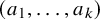
$(a_1,\dots ,a_k)$
and all sequences
$(a_1,\dots ,a_k)$
 of positive integers. We denote by
$\text{QSym}_{n}$
of positive integers. We denote by
$\text{QSym}_{n}$
 the ring of all quasisymmetric polynomials, and note that since the defining condition for quasisymmetry is a weakening of symmetry, the ring
$\operatorname {Sym}_{n}$
the ring of all quasisymmetric polynomials, and note that since the defining condition for quasisymmetry is a weakening of symmetry, the ring
$\operatorname {Sym}_{n}$
 of symmetric polynomials in
$\textbf {x}_n$
of symmetric polynomials in
$\textbf {x}_n$
 is a subring of
$\text{QSym}_{n}$
is a subring of
$\text{QSym}_{n}$
 .
.
In [Reference Aval, Bergeron and Bergeron4], Aval–Bergeron–Bergeron initiated the study of the
$\color {blue}{{quasisymmetric\, coinvariant\, ring}}$


The graded ring
$\operatorname {Coinv}_{n}:= \mathbb Z[\textbf {x}_n]/\operatorname {Sym}_{n}^+$
 has a unimodal symmetric sequence of ranks, which reflects the fact that
$H^{\bullet }(\mathrm {Fl}_{n})\simeq \operatorname {Coinv}_{n}$
has a unimodal symmetric sequence of ranks, which reflects the fact that
$H^{\bullet }(\mathrm {Fl}_{n})\simeq \operatorname {Coinv}_{n}$
 and
$\mathrm {Fl}_{n}$
and
$\mathrm {Fl}_{n}$
 is a smooth projective variety. In contrast, the graded space
$\text{QSCoinv}_{n}$
is a smooth projective variety. In contrast, the graded space
$\text{QSCoinv}_{n}$
 is not rank symmetric for any
$n\geq 3$
is not rank symmetric for any
$n\geq 3$
 [Reference Aval, Bergeron and Bergeron4, Theorem 1.1], and thus it cannot arise as the cohomology of any smooth projective variety.
We construct the quasisymmetric flag variety using a collection of
$(n-1)$
 -dimensional smooth toric varieties
$X(T)$
-dimensional smooth toric varieties
$X(T)$
 parameterized by the set
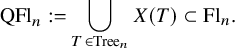
$\mathrm {Tree}_{n}$
parameterized by the set
$\mathrm {Tree}_{n}$
 of n-leaf planar binary trees,
Each variety
$X(T)$
 is a left-translated Richardson variety, and an iterated
$\mathbb {P}^1$
is a left-translated Richardson variety, and an iterated
$\mathbb {P}^1$
 -bundle following a process determined by the combinatorial structure of the tree T. The moment polytopes of these varieties are both combinatorial cubes and
$\color {blue}{{polypositroids}}$
-bundle following a process determined by the combinatorial structure of the tree T. The moment polytopes of these varieties are both combinatorial cubes and
$\color {blue}{{polypositroids}}$
 in the sense of Lam–Postnikov [Reference Lam and Postnikov33].
Theorem A. We have
$H^{\bullet }(\mathrm {QFl}_n)\cong \text{QSCoinv}_{n}$
 .
.
We note that this does not contradict the previous observation on smooth projective varieties as
$\mathrm {QFl}_n$
 is reducible. We give a similar presentation of the torus-equivariant cohomology ring via the coinvariant ring of the
$\color {blue}{{equivariantly\, quasisymmetric\, polynomials}}$
is reducible. We give a similar presentation of the torus-equivariant cohomology ring via the coinvariant ring of the
$\color {blue}{{equivariantly\, quasisymmetric\, polynomials}}$
 defined in [Reference Bergeron, Gagnon, Nadeau, Spink and Tewari6]; see Section 12.2.
The combinatorics of
$\mathrm {QFl}_n$
 is governed by
$\color {blue}{{noncrossing\, partitions}}$
is governed by
$\color {blue}{{noncrossing\, partitions}}$
 . Let
$S_{n}$
. Let
$S_{n}$
 denote the symmetric group on n letters. The torus fixed points of
$\mathrm {QFl}_{n}$
denote the symmetric group on n letters. The torus fixed points of
$\mathrm {QFl}_{n}$
 are exactly the permutations
$\operatorname {NC}_{n} \subseteq S_{n}$
are exactly the permutations
$\operatorname {NC}_{n} \subseteq S_{n}$
 obtained by treating each block of a noncrossing set partition as a backwards cycle; see Biane [Reference Biane9]. Noncrossing partitions also yield the following intrinsic characterization of
$\mathrm {QFl}_{n}$
obtained by treating each block of a noncrossing set partition as a backwards cycle; see Biane [Reference Biane9]. Noncrossing partitions also yield the following intrinsic characterization of
$\mathrm {QFl}_{n}$
 , which we prove in Section 10.
Theorem B. Denoting by
$[\mathrm {Pl}_{\sigma }]_{\sigma \in S_n}$
 the
$\color {blue}{{Pl\unicode{x00FC}cker\, functions}}$
the
$\color {blue}{{Pl\unicode{x00FC}cker\, functions}}$
 on
$\mathrm {Fl}_{n}$
on
$\mathrm {Fl}_{n}$
 , we have that

Our remaining results establish the following parallels between
$\mathrm {QFl}_{n}$
 and
$\mathrm {Fl}_{n}$
and
$\mathrm {Fl}_{n}$
 .
.
-
(1) The Bruhat decomposition gives a stratification of the flag variety into a union of affine Schubert cells $(X^w)^{\circ }$
 with well-behaved closure relations known as an affine paving. In Section 9, we describe an affine paving $$\begin{align*}\mathrm{QFl}_n = \bigsqcup_{w \in \operatorname{NC}_{n}} (X^{w})^{\circ} \cap \mathrm{QFl}_n, \end{align*}$$which shares many combinatorial properties with the Bruhat decomposition. In Section 11 we prove that the closures of our affine cells give a homology basis for $H_\bullet (\mathrm {QFl}_n)$
.
with well-behaved closure relations known as an affine paving. In Section 9, we describe an affine paving $$\begin{align*}\mathrm{QFl}_n = \bigsqcup_{w \in \operatorname{NC}_{n}} (X^{w})^{\circ} \cap \mathrm{QFl}_n, \end{align*}$$which shares many combinatorial properties with the Bruhat decomposition. In Section 11 we prove that the closures of our affine cells give a homology basis for $H_\bullet (\mathrm {QFl}_n)$
.
-
(2) Schubert polynomials [Reference Lascoux and Schützenberger34] give a basis of $H^{\bullet }(\mathrm {Fl}_{n})$
in Borel’s presentation, and this basis is Kronecker dual to the homology basis of Schubert cycles
$[X^w]$
. In Section 12 we prove that our homology basis is likewise Kronecker dual to the family of forest polynomials [Reference Nadeau and Tewari41, Reference Nadeau, Spink and Tewari39] and double forest polynomials [Reference Bergeron, Gagnon, Nadeau, Spink and Tewari6]. -
(3) The divided difference formalism for Schubert polynomials admits a geometric interpretation via Bott–Samelson resolutions of Schubert varieties. Forest polynomials satisfy similar formalisms, and we show in Section 12 that these operations can be similarly interpreted using iterated $\mathbb {P}^1$
-bundles. We exploit this connection to compute the degree map of each toric variety
$X(F)$
in
$\mathrm {QFl}_{n}$
using a recursive combinatorial process first defined in [Reference Bergeron, Gagnon, Nadeau, Spink and Tewari6]. -
(4) Torus-equivariant versions of (1)–(3) also hold, highlighting parallels between the classical double Schubert polynomials and the double forest polynomials defined in [Reference Bergeron, Gagnon, Nadeau, Spink and Tewari6].




In fact, many of our “nonequivariant” results are derived by first proving their equivariant analogue. In doing so, we rely crucially on the combinatorial relationship between double forest polynomials and noncrossing partitions developed in [Reference Bergeron, Gagnon, Nadeau, Spink and Tewari6]. In particular, we show that the Goresky–Kottwitz–MacPherson graph [Reference Goresky, Kottwitz and MacPherson25] associated to
$\mathrm {QFl}_n$
 under the standard torus action is the Kreweras lattice on
$\operatorname {NC}_{n}$
under the standard torus action is the Kreweras lattice on
$\operatorname {NC}_{n}$
 , and specializations of double forest polynomials describe a free basis of the associated graph cohomology ring. This generalizes earlier work of the first and second author [Reference Bergeron and Gagnon5] on
$\color {blue}{{quasisymmetric\, orbit\, harmonics}}$
, and specializations of double forest polynomials describe a free basis of the associated graph cohomology ring. This generalizes earlier work of the first and second author [Reference Bergeron and Gagnon5] on
$\color {blue}{{quasisymmetric\, orbit\, harmonics}}$
 , in which the main result shows that the ring

has associated graded
$\text{QSCoinv}_{n}$
 .
.
We now give a brief outline of the paper. In Section 2 we recall standard facts about
$\mathrm {Fl}_{n}$
 , noncrossing partitions, and binary trees. We then define a family of elementary “building operations” on
$\mathrm {Fl}_{n}$
, noncrossing partitions, and binary trees. We then define a family of elementary “building operations” on
$\mathrm {Fl}_{n}$
 in Section 3 and study the combinatorics of their compositions in Section 4. The building operations are the backbone of our work, and in Section 5 we use them to construct a family of Bott manifolds
$X(\widehat {F})$
in Section 3 and study the combinatorics of their compositions in Section 4. The building operations are the backbone of our work, and in Section 5 we use them to construct a family of Bott manifolds
$X(\widehat {F})$
 attached to bicolored nested forests
$\widehat {F}$
attached to bicolored nested forests
$\widehat {F}$
 that includes the
$X(T)$
that includes the
$X(T)$
 as the top-dimensional case. We provide a precise description of the inclusion order of these varieties in Section 6, highlighting the role of noncrossing partitions, and connect our work to Richardson varieties in Section 7. In Section 8 we define
$\mathrm {QFl}_{n}$
as the top-dimensional case. We provide a precise description of the inclusion order of these varieties in Section 6, highlighting the role of noncrossing partitions, and connect our work to Richardson varieties in Section 7. In Section 8 we define
$\mathrm {QFl}_{n}$
 and completely describe the structure of this complex. The final four sections (9, 10, 11, and 12) contain our main results, as described above.
In the remainder of this introduction, we explain the motivation behind the construction of the varieties
$X(T)$
 . In [Reference Nadeau, Spink and Tewari38] a partial solution to the geometric realization of
$\text{QSCoinv}_{n}$
. In [Reference Nadeau, Spink and Tewari38] a partial solution to the geometric realization of
$\text{QSCoinv}_{n}$
 was obtained via a different construction called the
$\color {blue}{\Omega{-}\textit{flag variety}}$
was obtained via a different construction called the
$\color {blue}{\Omega{-}\textit{flag variety}}$
 . Let
$S_{n-1}\subset S_n$
. Let
$S_{n-1}\subset S_n$
 comprise permutations w satisfying
$w(n)=n$
comprise permutations w satisfying
$w(n)=n$
 and denote the backwards long cycle
$\boldsymbol {c}=(n\, n-1\,\cdots \,1) \in S_n$
and denote the backwards long cycle
$\boldsymbol {c}=(n\, n-1\,\cdots \,1) \in S_n$
 . In [Reference Nadeau, Spink and Tewari38], the third, fourth, and fifth authors consider the complex of
$(n-1)!$
. In [Reference Nadeau, Spink and Tewari38], the third, fourth, and fifth authors consider the complex of
$(n-1)!$
 smooth toric Richardson varieties
under the torus action of
$T_n=(\mathbb {C}^*)^n$
 acting on
$\mathrm {Fl}_{n}$
acting on
$\mathrm {Fl}_{n}$
 via its action on
$\mathbb {C}^n$
via its action on
$\mathbb {C}^n$
 . This complex was first studied in [Reference Harada, Horiguchi, Masuda and Park29, Reference Lian36] as arising from a toric degeneration of a general
$T_n$
. This complex was first studied in [Reference Harada, Horiguchi, Masuda and Park29, Reference Lian36] as arising from a toric degeneration of a general
$T_n$
 -orbit closure in
$\mathrm {Fl}_{n}$
-orbit closure in
$\mathrm {Fl}_{n}$
 . We emphasize that this complex differs from
$\mathrm {QFl}_n$
. We emphasize that this complex differs from
$\mathrm {QFl}_n$
 , as for
$n\ge 3$
, as for
$n\ge 3$
 it contains more Richardson varieties than there are
$X(T)$
it contains more Richardson varieties than there are
$X(T)$
 varieties. Each toric Richardson in this complex is smooth and has a moment polytope that is a combinatorial cube.
The toric complex
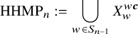
$\operatorname {HHMP}_n$
 is assembled in a combinatorially simple way, equivalent to the decomposition of
$[0, 1] \times [0, 2] \times \cdots \times [0, n-1]$
is assembled in a combinatorially simple way, equivalent to the decomposition of
$[0, 1] \times [0, 2] \times \cdots \times [0, n-1]$
 into unit cubes; see [Reference Nadeau, Spink and Tewari38, Section 7.1]. One of the main results of [Reference Nadeau, Spink and Tewari38] was that for the inclusion
$\phi \colon \operatorname {HHMP}_n\to \mathrm {Fl}_{n}$
into unit cubes; see [Reference Nadeau, Spink and Tewari38, Section 7.1]. One of the main results of [Reference Nadeau, Spink and Tewari38] was that for the inclusion
$\phi \colon \operatorname {HHMP}_n\to \mathrm {Fl}_{n}$
 , we have

Here the inclusion is strict: multiple cycles
$X^{w\boldsymbol {c}}_w$
 are equivalent under the left action of
$S_n$
are equivalent under the left action of
$S_n$
 by permutation matrices.
The geometry of
$\mathrm {QFl}_n$
 is constructed to avoid this duplication problem. We show (see also [Reference Nadeau, Spink and Tewari38, §6]) that the
$X(T)$
is constructed to avoid this duplication problem. We show (see also [Reference Nadeau, Spink and Tewari38, §6]) that the
$X(T)$
 varieties collapse the left-translation redundancy of the
$X^{w\boldsymbol {c}}_w$
varieties collapse the left-translation redundancy of the
$X^{w\boldsymbol {c}}_w$
 via a surjective map

taking the
$(n-1)!$
 -many Richardson varieties to the
$\operatorname {Cat}_{n-1}=\frac {1}{n}\binom {2n-2}{n-1}$
-many Richardson varieties to the
$\operatorname {Cat}_{n-1}=\frac {1}{n}\binom {2n-2}{n-1}$
 -many
$X(T)$
-many
$X(T)$
 varieties.
The trade-off in the construction of
$\mathrm {QFl}_{n}$
 is a more complicated toric complex. In particular, the moment polytopes of our translated Richardson varieties overlap in an irregular manner, and torus orbits associated to partially overlapping faces do not intersect. These phenomena first appear in the case
$n = 3$
is a more complicated toric complex. In particular, the moment polytopes of our translated Richardson varieties overlap in an irregular manner, and torus orbits associated to partially overlapping faces do not intersect. These phenomena first appear in the case
$n = 3$
 , and Figure 1 contrasts the structure of the moment polytopes for
$\operatorname {HHMP}_{n}$
, and Figure 1 contrasts the structure of the moment polytopes for
$\operatorname {HHMP}_{n}$
 with our “translated” moment polytopes, which reflects the structure of
$\mathrm {QFl}_{n}$
with our “translated” moment polytopes, which reflects the structure of
$\mathrm {QFl}_{n}$
 . Geometrically,
$\operatorname {HHMP}_3$
. Geometrically,
$\operatorname {HHMP}_3$
 is two Hirzebruch surfaces glued along a common torus-invariant
$\mathbb {P}^1$
is two Hirzebruch surfaces glued along a common torus-invariant
$\mathbb {P}^1$
 , while
$\mathrm {QFl}_3$
, while
$\mathrm {QFl}_3$
 is two Hirzebruch surfaces glued along two different and intersecting torus-invariant
$\mathbb {P}^1$
is two Hirzebruch surfaces glued along two different and intersecting torus-invariant
$\mathbb {P}^1$
 ’s. We revisit this figure in Section 8 where the right panel is redrawn to resemble the Kreweras lattice
$\operatorname {NC}_3$
’s. We revisit this figure in Section 8 where the right panel is redrawn to resemble the Kreweras lattice
$\operatorname {NC}_3$
 .
.
The two trapezoids comprising the HHMP subdivision of the
$n=3$
 permutahedron (left) and the intersecting
$X(T)$
permutahedron (left) and the intersecting
$X(T)$
 moment polytopes (right).
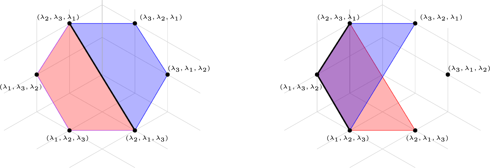
Figure 1 Long description
The diagram consists of two panels set against a light gray isometric grid.
Left panel: A hexagonal shape is divided into two trapezoids by a thick black diagonal line. The left trapezoid is shaded red and the right trapezoid is shaded blue. The vertices are labeled with lambda coordinates. Starting from the top left and moving clockwise, the labels are (lambda sub 2, lambda sub 3, lambda sub 1), (lambda sub 3, lambda sub 2, lambda sub 1), (lambda sub 3, lambda sub 1, lambda sub 2), (lambda sub 2, lambda sub 1, lambda sub 3), (lambda sub 1, lambda sub 2, lambda sub 3), and (lambda sub 1, lambda sub 3, lambda sub 2). The dividing line connects (lambda sub 2, lambda sub 3, lambda sub 1) to (lambda sub 2, lambda sub 1, lambda sub 3).
Right panel: The same hexagonal frame is shown, but the internal shapes are different. A blue triangle and a red triangle overlap to form a purple intersection. The blue triangle has vertices at (lambda sub 2, lambda sub 3, lambda sub 1), (lambda sub 3, lambda sub 2, lambda sub 1), and (lambda sub 1, lambda sub 2, lambda sub 3). The red triangle has vertices at (lambda sub 1, lambda sub 3, lambda sub 2), (lambda sub 2, lambda sub 1, lambda sub 3), and a point near the top center. A thick black line highlights the left edge of the purple overlapping region between (lambda sub 2, lambda sub 3, lambda sub 1) and (lambda sub 1, lambda sub 2, lambda sub 3). The vertex (lambda sub 3, lambda sub 1, lambda sub 2) remains as an isolated point on the far right.
2 Preliminaries
Let
$s_1,\ldots ,s_{n-1}$
 be the simple transpositions
$s_i=(i,i+1)$
be the simple transpositions
$s_i=(i,i+1)$
 generating the symmetric group
$S_n$
generating the symmetric group
$S_n$
 . We let

denote the backwards long cycle. For all nonnegative integers m we set
$[m]:= \{1,\dots ,m\}$
 .
.
2.1 Recollections on
$\mathrm {Fl}_{n}$

We work over
$\mathbb C$
 and denote by
$T_{n},B_{n},B_{n}^-\subset \mathrm {GL}_{n}$
and denote by
$T_{n},B_{n},B_{n}^-\subset \mathrm {GL}_{n}$
 the subsets of diagonal, upper triangular, and lower triangular invertible
$n\times n$
the subsets of diagonal, upper triangular, and lower triangular invertible
$n\times n$
 matrices. When there is no ambiguity we write T, B, and
$B^-$
matrices. When there is no ambiguity we write T, B, and
$B^-$
 for
$T_{n}$
for
$T_{n}$
 ,
$B_{n}$
,
$B_{n}$
 , and
$B^{-}_{n}$
, and
$B^{-}_{n}$
 . We will denote by
$\chi _i$
. We will denote by
$\chi _i$
 the i-th standard character of
$T_n$
the i-th standard character of
$T_n$
 , corresponding to the i-th entry along the diagonal, so that for
$a = \mathrm {diag}(a_{1}, \ldots , a_{n}) \in T$
, corresponding to the i-th entry along the diagonal, so that for
$a = \mathrm {diag}(a_{1}, \ldots , a_{n}) \in T$
 we have
$\chi _{i}(a) = a_{i}$
we have
$\chi _{i}(a) = a_{i}$
 . For
$\chi $
. For
$\chi $
 a character of T, we will denote by
$\mathbb {C}_{\chi }$
a character of T, we will denote by
$\mathbb {C}_{\chi }$
 the corresponding
$1$
the corresponding
$1$
 -dimensional representation.
We identify the complete flag variety

with
$\mathrm {GL}_{n}/B_{n}$
 via the transitive action of
$\mathrm {GL}_{n}$
via the transitive action of
$\mathrm {GL}_{n}$
 with
$B_{n}$
with
$B_{n}$
 the stabilizer of the
$\color {blue}{{standard\, coordinate\, flag}}$
the stabilizer of the
$\color {blue}{{standard\, coordinate\, flag}}$
 with
$\mathcal {F}_i=\langle e_1,\ldots ,e_i\rangle$
with
$\mathcal {F}_i=\langle e_1,\ldots ,e_i\rangle$
 for
$1\leq i\leq n$
for
$1\leq i\leq n$
 . Via this identification the i-th subspace in the flag associated to
$hB_{n}$
. Via this identification the i-th subspace in the flag associated to
$hB_{n}$
 is the column span of the first i columns of h for
$1\leq i\leq n$
is the column span of the first i columns of h for
$1\leq i\leq n$
 .
.
For
$w \in S_{n}$
 , we will denote the Schubert cycles in
$\mathrm {Fl}_{n}$
, we will denote the Schubert cycles in
$\mathrm {Fl}_{n}$
 by
$X^v=\overline {BvB}$
by
$X^v=\overline {BvB}$
 , the opposite Schubert cycles by
$X_u=\overline {B^-uB}$
, the opposite Schubert cycles by
$X_u=\overline {B^-uB}$
 , and for
$u\le v$
, and for
$u\le v$
 in the Bruhat order the Richardson varieties
$X^v_u:= X^v\cap X_u=\overline {BvB}\cap \overline {B^-uB}$
in the Bruhat order the Richardson varieties
$X^v_u:= X^v\cap X_u=\overline {BvB}\cap \overline {B^-uB}$
 . The Bruhat decomposition

gives an affine paving if the
$BwB$
 are ordered via any linear extension of the Bruhat order on
$S_n$
are ordered via any linear extension of the Bruhat order on
$S_n$
 ; see Section 9 for more details.
For
$w \in S_{n}$
 and a dominant weight
$\lambda =(\lambda _1\ge \cdots \ge \lambda _n)\in \mathbb {Z}^n$
and a dominant weight
$\lambda =(\lambda _1\ge \cdots \ge \lambda _n)\in \mathbb {Z}^n$
 , we have a
$\color {blue}{{Pl\unicode{x00FC}cker\, function}}$
, we have a
$\color {blue}{{Pl\unicode{x00FC}cker\, function}}$
 defined for
$h\in \mathrm {GL}_n$
defined for
$h\in \mathrm {GL}_n$
 by
by

where
$h_{i_1,\ldots ,i_k}$
 is the submatrix of h with columns
$1,\ldots ,k$
is the submatrix of h with columns
$1,\ldots ,k$
 and rows
$i_1,\ldots ,i_k$
and rows
$i_1,\ldots ,i_k$
 . These functions together define a map
$\mathrm {Pl}_{\lambda }:\mathrm {Fl}_{n}\to \mathbb {P}^{n!-1}$
. These functions together define a map
$\mathrm {Pl}_{\lambda }:\mathrm {Fl}_{n}\to \mathbb {P}^{n!-1}$
 , which we write simply
$\mathrm {Pl}$
, which we write simply
$\mathrm {Pl}$
 if
$\lambda $
if
$\lambda $
 is the fundamental dominant weight
${(n,n-1,\ldots ,1)}$
is the fundamental dominant weight
${(n,n-1,\ldots ,1)}$
 . Then
$\mathrm {Pl}_{\lambda }$
. Then
$\mathrm {Pl}_{\lambda }$
 is
$T_n$
is
$T_n$
 -equivariant with respect to the
$T_n$
-equivariant with respect to the
$T_n$
 -action on
$\mathbb {P}^{n!-1}$
-action on
$\mathbb {P}^{n!-1}$
 where
$\mathrm {diag}(a_1,\ldots ,a_n)\in T_n$
where
$\mathrm {diag}(a_1,\ldots ,a_n)\in T_n$
 acts in the w-coordinate by
$a_{w(1)}^{\lambda _1}a_{w(2)}^{\lambda _2}\cdots a_{w(n)}^{\lambda _n}=a_1^{\lambda _{w^{-1}(1)}}\cdots a_n^{\lambda _{w^{-1}(n)}}$
acts in the w-coordinate by
$a_{w(1)}^{\lambda _1}a_{w(2)}^{\lambda _2}\cdots a_{w(n)}^{\lambda _n}=a_1^{\lambda _{w^{-1}(1)}}\cdots a_n^{\lambda _{w^{-1}(n)}}$
 .
.
The moment polytope of
$\mathrm {Fl}_{n}$
 under
$\mathrm {Pl}_{\lambda }$
under
$\mathrm {Pl}_{\lambda }$
 is the generalized permutahedron

where
$u\cdot {\lambda } = (\lambda _{u^{-1}(1)},\ldots ,\lambda _{u^{-1}(n)})$
 and
$\operatorname {conv}$
and
$\operatorname {conv}$
 denotes taking the convex hull. If
$X\subset \mathrm {Fl}_{n}$
denotes taking the convex hull. If
$X\subset \mathrm {Fl}_{n}$
 is a
$T_n$
is a
$T_n$
 -invariant subvariety, then its moment polytope under
$\mathrm {Pl}_{\lambda }$
-invariant subvariety, then its moment polytope under
$\mathrm {Pl}_{\lambda }$
 is
is

The moment polytope of a
$T_{n}$
 -orbit closure X is always a
$\color {blue}{{flag\ matroid\ polytope}}$
-orbit closure X is always a
$\color {blue}{{flag\ matroid\ polytope}}$
 (see [Reference Gelfand, Goresky, MacPherson and Serganova22]), meaning its vertices are contained in the vertices of
$\operatorname {Perm}(\lambda )$
(see [Reference Gelfand, Goresky, MacPherson and Serganova22]), meaning its vertices are contained in the vertices of
$\operatorname {Perm}(\lambda )$
 and all edges are parallel to the type
$A_{n-1}$
and all edges are parallel to the type
$A_{n-1}$
 roots
$e_i-e_j$
roots
$e_i-e_j$
 for various
$i,j$
for various
$i,j$
 .
.
2.2 Noncrossing partitions
A
$\color {blue}{{combinatorial\, noncrossing\, partition}}$
 is a partition
$A_1\sqcup \cdots \sqcup A_k=[n]$
is a partition
$A_1\sqcup \cdots \sqcup A_k=[n]$
 such that for
$i\ne j$
such that for
$i\ne j$
 , distinct elements
$a,b\in A_i$
, distinct elements
$a,b\in A_i$
 , and distinct elements
$c,d\in A_j$
, and distinct elements
$c,d\in A_j$
 , we never have
$a<c<b<d$
, we never have
$a<c<b<d$
 . We depict combinatorial noncrossing partitions as noncrossing arc diagrams; for example we draw
$\{1,2,3,6\}\sqcup \{4,5\}=[6]$
. We depict combinatorial noncrossing partitions as noncrossing arc diagrams; for example we draw
$\{1,2,3,6\}\sqcup \{4,5\}=[6]$
 as
as

A
$\color {blue}{{backwards\, cycle}}$
 is a cycle
$(b_1\,b_2\,\cdots \, b_r)$
is a cycle
$(b_1\,b_2\,\cdots \, b_r)$
 with
$b_1>b_2>\cdots >b_r$
with
$b_1>b_2>\cdots >b_r$
 . An
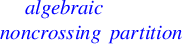
$\color {blue}{{algebraic}} \color {blue}{{noncrossing\, partition}}$
. An
$\color {blue}{{algebraic}} \color {blue}{{noncrossing\, partition}}$
 is defined to be a permutation w whose disjoint cycle decomposition
$\operatorname {Cyc}(w):= C_{1}C_{2} \cdots C_{k}$
is defined to be a permutation w whose disjoint cycle decomposition
$\operatorname {Cyc}(w):= C_{1}C_{2} \cdots C_{k}$
 consists of backwards cycles whose underlying sets define a combinatorial noncrossing partition. For example,
$w = (6321)(54)$
consists of backwards cycles whose underlying sets define a combinatorial noncrossing partition. For example,
$w = (6321)(54)$
 is the algebraic noncrossing partition associated to the arc diagram above. We denote

The
$\color {blue}{{Kreweras\, order}}$
 on
$\operatorname {NC}_n$
on
$\operatorname {NC}_n$
 is defined by setting
$u\le _K v$
is defined by setting
$u\le _K v$
 if the combinatorial noncrossing partition associated to u refines the combinatorial noncrossing partition associated to v. For example,
$(63)(21)(54)\le _K (6321)(54)$
if the combinatorial noncrossing partition associated to u refines the combinatorial noncrossing partition associated to v. For example,
$(63)(21)(54)\le _K (6321)(54)$
 . The Kreweras order is a lattice, and the lattice structure is induced by the lattice of set partitions under refinement [Reference Kreweras32].
Going forward, we will identify combinatorial and algebraic noncrossing partitions, using “combinatorial” and “algebraic” only when disambiguation is needed.
We say that permutations
$u,w\in S_n$
 are
$\color {blue}{{adjacent}}$
are
$\color {blue}{{adjacent}}$
 if
$w=(i\,j)u$
if
$w=(i\,j)u$
 for some transposition
$(i\,j)$
for some transposition
$(i\,j)$
 . Let
$\operatorname {Cayley}(S_n)$
. Let
$\operatorname {Cayley}(S_n)$
 be the
$\color {blue}{{Cayley\, graph}}$
be the
$\color {blue}{{Cayley\, graph}}$
 on
$S_n$
on
$S_n$
 in which adjacent permutations are connected by an edge. Then
$u,w\in \operatorname {NC}_n$
in which adjacent permutations are connected by an edge. Then
$u,w\in \operatorname {NC}_n$
 are adjacent in the Kreweras lattice (meaning one element covers the other) if and only if
$u,w$
are adjacent in the Kreweras lattice (meaning one element covers the other) if and only if
$u,w$
 are adjacent in
$\operatorname {Cayley}(S_n)$
are adjacent in
$\operatorname {Cayley}(S_n)$
 . In this way, we may identify the Hasse diagram of the Kreweras lattice with the induced subgraph of
$\operatorname {Cayley}(S_n)$
. In this way, we may identify the Hasse diagram of the Kreweras lattice with the induced subgraph of
$\operatorname {Cayley}(S_n)$
 on
$\operatorname {NC}_n$
on
$\operatorname {NC}_n$
 as was first observed by Biane [Reference Biane9]. We denote this induced subgraph by
$\operatorname {Cayley}(\operatorname {NC}_{n})$
as was first observed by Biane [Reference Biane9]. We denote this induced subgraph by
$\operatorname {Cayley}(\operatorname {NC}_{n})$
 .
.
Remark 2.1. The Kreweras order is different from the Bruhat order
$\le $
 restricted to
$\operatorname {NC}_n$
restricted to
$\operatorname {NC}_n$
 . For example,
$\boldsymbol {c}$
. For example,
$\boldsymbol {c}$
 is the maximal element of
$\le _K$
is the maximal element of
$\le _K$
 , whereas the longest element
$w_o\in S_n$
, whereas the longest element
$w_o\in S_n$
 , which is also in
$\mathrm {NC}_n$
, which is also in
$\mathrm {NC}_n$
 , is the maximal element of
$\le $
, is the maximal element of
$\le $
 . See [Reference Biane and Josuat-Vergès10] for a more detailed study of the interaction between the two orders.
2.3 Binary trees and nested forests
A
$\color {blue}{{planar\, binary\, tree}}$
 is a rooted tree T in which each node v is either an
$\color {blue}{{internal\, node}}$
is a rooted tree T in which each node v is either an
$\color {blue}{{internal\, node}}$
 with exactly
$2$
with exactly
$2$
 children
$v_L$
children
$v_L$
 and
$v_R$
and
$v_R$
 (the left and right children), or v is a
$\color {blue}{{leaf}}$
(the left and right children), or v is a
$\color {blue}{{leaf}}$
 with zero children. Let
$\operatorname {IN}(T)$
with zero children. Let
$\operatorname {IN}(T)$
 denote the set of internal nodes in T. We allow for the possibility that
$|\operatorname {IN}(T)|=0$
denote the set of internal nodes in T. We allow for the possibility that
$|\operatorname {IN}(T)|=0$
 , in which case the unique node is both a root and a leaf.
A
$\color {blue}{{nested\, forest\, supported\, on\, [n]}}$
 is a family
$\widehat {F} = (T_{C})_{C \in \operatorname {Cyc}(w)}$
is a family
$\widehat {F} = (T_{C})_{C \in \operatorname {Cyc}(w)}$
 of binary trees
$T_{C}$
of binary trees
$T_{C}$
 indexed by the disjoint cycles of a noncrossing partition
$w = C_{1} C_{2} \cdots C_{k} \in \operatorname {NC}_{n}$
indexed by the disjoint cycles of a noncrossing partition
$w = C_{1} C_{2} \cdots C_{k} \in \operatorname {NC}_{n}$
 such that each
$T_{C}$
such that each
$T_{C}$
 has
$|C|$
has
$|C|$
 leaves. We identify the leaves of each
$T_{C}$
leaves. We identify the leaves of each
$T_{C}$
 with the underlying set of C in increasing order and depict
$\widehat {F}$
with the underlying set of C in increasing order and depict
$\widehat {F}$
 by drawing the
$T_{C}$
by drawing the
$T_{C}$
 in the upper half plane so that the set
$[n]$
in the upper half plane so that the set
$[n]$
 of all leaves appears in increasing order along the horizontal axis.
The internal nodes of
$\widehat {F}$
 are
$\operatorname {IN}(\widehat {F}) = \bigsqcup _{C \in \operatorname {Cyc}(w)} \operatorname {IN}(T_{C})$
are
$\operatorname {IN}(\widehat {F}) = \bigsqcup _{C \in \operatorname {Cyc}(w)} \operatorname {IN}(T_{C})$
 . The
$\color {blue}{{canonical\, label}}$
. The
$\color {blue}{{canonical\, label}}$
 of each
$v \in \operatorname {IN}(\widehat {F})$
of each
$v \in \operatorname {IN}(\widehat {F})$
 is the value of the rightmost leaf descendant of
$v_L$
is the value of the rightmost leaf descendant of
$v_L$
 . See, for example, Figure 2 (left).
A nested forest with its canonical labeling in red (left) and the underlying noncrossing partition in cycle notation (right).

We define a map
$\operatorname {NCPerm}: \operatorname {NestFor}_{n} \to \operatorname {NC}_{n}$
 that sends a nested forest
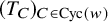
$(T_{C})_{C \in \operatorname {Cyc}(w)}$
that sends a nested forest
$(T_{C})_{C \in \operatorname {Cyc}(w)}$
 to its underlying noncrossing partition
$w=\prod _{C\in \operatorname {Cyc}(w)}C$
to its underlying noncrossing partition
$w=\prod _{C\in \operatorname {Cyc}(w)}C$
 . See, for example, Figure 2 (right).
Remark 2.2. Nested forests should be seen as an enriched version of noncrossing partitions. In Section 6, we show that each nested forest corresponds, up to certain trivial commutation relations, to a distinguished factorization of its associated noncrossing partition.
3 Building split
$\mathbb {P}^1$
-bundles

We now introduce the operations used to build
$\mathrm {QFl}_n\subset \mathrm {Fl}_{n}$
 .
.
3.1
$\Psi _i^-$
and
$\Psi _i^+$


We recall certain pattern maps that were studied by Bergeron–Sottile [Reference Bergeron and Sottile7] and summarize their essential properties. We refer the reader to [Reference Billey and Braden13, Reference Billey and Postnikov11] for a more general perspective. Throughout, let
$\operatorname {Mat}_{a\times b}$
 be the set of
$a\times b$
be the set of
$a\times b$
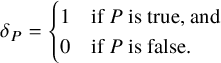
 matrices and, for a property P, define
Definition 3.1. Let
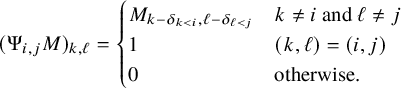
$\Psi _{i,j}\colon \operatorname {Mat}_{m-1\times m-1}\to \operatorname {Mat}_{m\times m}$
 be the operation
The map
$\Psi _{1,i}$
 was crucial to the construction in [Reference Nadeau, Spink and Tewari38, §5]. In contrast, the following two pattern maps will be important to us:

For example, when
$m=4$
 we have
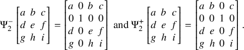
By restricting to invertible matrices, the pattern maps descend to closed embeddings

Define
$\gamma _i:T_m\to T_{m-1}$
 to be the map
$\mathrm {diag}(a_1,\ldots ,a_{m})\mapsto \mathrm {diag}(a_1,\ldots ,a_{i-1},a_{i+1},\ldots ,a_{m})$
to be the map
$\mathrm {diag}(a_1,\ldots ,a_{m})\mapsto \mathrm {diag}(a_1,\ldots ,a_{i-1},a_{i+1},\ldots ,a_{m})$
 .
.
Definition 3.2. If T is a torus and
$\gamma :T\to T_m$
 is a map of tori then we write
$\mathrm {Fl}_{m}^\gamma $
is a map of tori then we write
$\mathrm {Fl}_{m}^\gamma $
 for
$\mathrm {Fl}_{m}$
for
$\mathrm {Fl}_{m}$
 equipped with the action of T induced by
$\gamma $
equipped with the action of T induced by
$\gamma $
 .
.
Fact 3.3. The maps
$\Psi _{i,j}:\mathrm {Fl}_{m-1}^{\gamma _i}\to \mathrm {Fl}_{m}$
 are
$T_m$
are
$T_m$
 -equivariant closed embeddings, and in particular this is true of
$\Psi _i^{\pm }:\mathrm {Fl}_{m-1}^{\gamma _i}\hookrightarrow \mathrm {Fl}_{m}$
-equivariant closed embeddings, and in particular this is true of
$\Psi _i^{\pm }:\mathrm {Fl}_{m-1}^{\gamma _i}\hookrightarrow \mathrm {Fl}_{m}$
 .
.
Write
$\epsilon _{i}:\mathbb {C}^{m-1}\hookrightarrow \mathbb {C}^{m}$
 for the inclusion
$(x_1,\ldots ,x_{m-1})\mapsto (x_1,\ldots ,x_{i-1},0,x_i,\ldots ,x_{m-1})$
for the inclusion
$(x_1,\ldots ,x_{m-1})\mapsto (x_1,\ldots ,x_{i-1},0,x_i,\ldots ,x_{m-1})$
 . Then
$\epsilon _i$
. Then
$\epsilon _i$
 is a
$T_m$
is a
$T_m$
 -equivariant inclusion if we give
$\mathbb {C}^{m-1}$
-equivariant inclusion if we give
$\mathbb {C}^{m-1}$
 the action of
$T_m$
the action of
$T_m$
 induced by
$\gamma _i$
induced by
$\gamma _i$
 , and we have

3.2 Building
$\mathbb P^1$
-bundles with
$\mathbb P_i$


We use the subbundle convention for relative projectivization, so that for
$\mathcal {V}$
 a vector bundle on a variety X we have
$\mathsf {Proj}(\mathcal {V})_X:=(\mathcal {V}\setminus \{0\})/\mathbb {C}^*$
a vector bundle on a variety X we have
$\mathsf {Proj}(\mathcal {V})_X:=(\mathcal {V}\setminus \{0\})/\mathbb {C}^*$
 . Consider the sequence of maps

where
$P_i$
 is the minimal parabolic subgroup of
$\mathrm {GL}_{m}$
is the minimal parabolic subgroup of
$\mathrm {GL}_{m}$
 containing
$s_i$
containing
$s_i$
 , and
$\pi _i$
, and
$\pi _i$
 is the projection map.
The space
$\mathrm {GL}_m/P_i$
 is typically identified with the variety of partial flags
$\{0\}\subset \mathcal {F}_1\subset \cdots \subset \mathcal {F}_{i-1}\subset \mathcal {F}_{i+1}\subset \cdots \subset \mathcal {F}_m=\mathbb {C}^m$
is typically identified with the variety of partial flags
$\{0\}\subset \mathcal {F}_1\subset \cdots \subset \mathcal {F}_{i-1}\subset \mathcal {F}_{i+1}\subset \cdots \subset \mathcal {F}_m=\mathbb {C}^m$
 with
$\dim \mathcal {F}_j=j$
with
$\dim \mathcal {F}_j=j$
 . Under this identification
$\pi _i$
. Under this identification
$\pi _i$
 becomes the map that forgets the i-th subspace of a complete flag.
Fact 3.4.
$\mathrm {Fl}_{m}\to \mathrm {GL}_m/P_i$
 is
$T_m$
is
$T_m$
 -equivariantly isomorphic to the
$\mathbb {P}^1$
-equivariantly isomorphic to the
$\mathbb {P}^1$
 -bundle
$\mathsf {Proj}(\mathcal {F}_{i+1}/\mathcal {F}_{i-1})_{\mathrm {GL}_{m}/P_i}$
-bundle
$\mathsf {Proj}(\mathcal {F}_{i+1}/\mathcal {F}_{i-1})_{\mathrm {GL}_{m}/P_i}$
 .
.
We now study how the
$\mathbb P^1$
 -bundle
$\pi _i$
-bundle
$\pi _i$
 interacts with the maps
$\Psi _i^{\pm }$
interacts with the maps
$\Psi _i^{\pm }$
 . Since
$s_{i}P_{i} = P_{i}$
. Since
$s_{i}P_{i} = P_{i}$
 , we have the equality
$\pi _i\Psi _i^-=\pi _i\Psi _i^+.$
, we have the equality
$\pi _i\Psi _i^-=\pi _i\Psi _i^+.$
 Consequently we write

to emphasize that this composite does not depend on
$\pm $
 . The map
$\pi _i\Psi _i$
. The map
$\pi _i\Psi _i$
 is given by
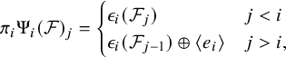
and is a closed
$T_m$
 -equivariant embedding
$\mathrm {Fl}_{m-1}^{\gamma _i}\hookrightarrow \mathrm {GL}_m/P_i$
-equivariant embedding
$\mathrm {Fl}_{m-1}^{\gamma _i}\hookrightarrow \mathrm {GL}_m/P_i$
 with image

For
$Z\subset \mathrm {Fl}_{m-1}$
 , we define a map

We now describe
$\mathbb {P}_iZ$
 using matrix representatives. For an
$(m-1)\times (m-1)$
using matrix representatives. For an
$(m-1)\times (m-1)$
 matrix M, let
$\mathbb {G}_iM$
matrix M, let
$\mathbb {G}_iM$
 be the set of all
$m \times m$
be the set of all
$m \times m$
 matrices obtained from
$\Psi _i^+M$
matrices obtained from
$\Psi _i^+M$
 by replacing the
$0$
by replacing the
$0$
 in entry
$(i,i)$
in entry
$(i,i)$
 with any value
$+ \in \mathbb {C}^*$
with any value
$+ \in \mathbb {C}^*$
 . The construction of
$\mathbb {G}_i$
. The construction of
$\mathbb {G}_i$
 commutes with forward column operations and therefore descends to a map
$\{\text {subsets of } \mathrm {Fl}_{m-1}\}\to \{\text {subsets of } \mathrm {Fl}_{m}\}$
commutes with forward column operations and therefore descends to a map
$\{\text {subsets of } \mathrm {Fl}_{m-1}\}\to \{\text {subsets of } \mathrm {Fl}_{m}\}$
 , and
$\mathbb {P}_iZ=(\Psi _i^+Z)\sqcup (\mathbb {G}_iZ)\sqcup (\Psi _i^-Z)$
, and
$\mathbb {P}_iZ=(\Psi _i^+Z)\sqcup (\mathbb {G}_iZ)\sqcup (\Psi _i^-Z)$
 . For example, when
$m=4$
. For example, when
$m=4$
 we have

Theorem 3.5. Let
$Z\subset \mathrm {Fl}_{m-1}$
 be a
$T_{m-1}$
be a
$T_{m-1}$
 -invariant subvariety. If we consider Z as a
$T_m$
-invariant subvariety. If we consider Z as a
$T_m$
 -invariant subvariety of
$\mathrm {Fl}_{m-1}^{\gamma _i}$
-invariant subvariety of
$\mathrm {Fl}_{m-1}^{\gamma _i}$
 for some fixed
$1\le i \le m-1$
for some fixed
$1\le i \le m-1$
 , then the following are true.
-
1. The map
$$ \begin{align*}(\pi_i\Psi_i)^{-1} \pi_i\colon \mathbb P_iZ\to Z\end{align*} $$realizes $\mathbb P_i Z$
as a
$T_m$
-equivariant
$\mathbb P^1$
-bundle over Z, which is
$T_m$
-equivariantly isomorphic to the
$\mathbb {P}^1$
-bundle
$\mathsf {Proj}((\mathcal {F}_i/\mathcal {F}_{i-1})\oplus \mathbb C_{\chi _i})_Z\to Z$
.
-
2. The closed subsets $\Psi _i^-|_Z$
and
$\Psi _i^+|_Z$
correspond to the
$T_m$
-equivariant sections
$\mathsf {Proj}(\{0\}\oplus \mathbb C_{\chi _i})_Z$
and
$\mathsf {Proj}((\mathcal {F}_i/\mathcal {F}_{i-1})\oplus \{0\})_Z$
respectively.








Proof. Both results follow from the case
$Z=\mathrm {Fl}_{m-1}$
 by restriction, so we consider only
$Z=\mathrm {Fl}_{m-1}$
by restriction, so we consider only
$Z=\mathrm {Fl}_{m-1}$
 .
.
-
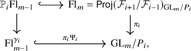
1. Since $\mathbb {P}_i\mathrm {Fl}_{m-1}$
can be defined by the pullback diagram we have that $\mathbb {P}_i\mathrm {Fl}_{m-1}$
is the projectivization of the pullback of
$\mathcal {F}_{i+1}/\mathcal {F}_{i-1}$
under the closed embedding
$\pi _i\Psi _i$
. This pullback is given by (3.1) $$ \begin{align} (\pi_i\Psi_i)^*(\mathcal{F}_{i+1}/\mathcal{F}_{i-1})=(\mathcal{F}_i\oplus \mathbb{C}_{\chi_i}) /(\mathcal{F}_{i-1}\oplus \{0\})\cong (\mathcal{F}_{i}/\mathcal{F}_{i-1})\oplus \mathbb C_{\chi_i}\end{align} $$so the result follows.
-
2. We can realize $\Psi _i^-\mathrm {Fl}_{m-1}$
and
$\Psi _i^+\mathrm {Fl}_{m-1}$
as
$T_m$
-equivariant sections of
$\pi _i|_{\mathbb {P}_i\mathrm {Fl}_{m-1}}$
taking a partial flag
$\{\mathcal {F}_j\}_{j\in [m]\setminus i}\in \pi _i\Psi _i(\mathrm {Fl}_{m-1})$
to respectively $$ \begin{align*} &\{0\}\subset \mathcal{F}_1\subset \cdots \subset \mathcal{F}_{i-1}\subset \mathcal{F}_{i-1}\oplus \langle e_i\rangle \subset \mathcal{F}_{i+1}\subset \cdots \subset \mathcal{F}_{m-1}\subset \mathbb C^{m},\text{ and}\\ &\{0\}\subset \mathcal{F}_1\subset \cdots \subset \mathcal{F}_{i-1}\subset \mathcal{F}_{i+1} \cap \{x_i=0\}\subset \mathcal{F}_{i+1}\subset \cdots \subset \mathcal{F}_{m-1}\subset \mathbb C^{m}. \end{align*} $$These two sections correspond to the choice of intermediate sub-bundles $\mathcal {F}_{i-1}{\kern-1pt}\oplus{\kern-1pt} \langle e_i\rangle$
and
${\mathcal {F}_{i+1}{\kern-1pt}\cap{\kern-0pt} \{x_i{\kern-1pt}={\kern-1pt}0\}}$
between
$\mathcal {F}_{i-1}|_{\pi _i\Psi _i(\mathrm {Fl}_{m-1})}$
and
$\mathcal {F}_{i+1}|_{\pi _i\Psi _i(\mathrm {Fl}_{m-1})}$
, which in the pullback bundle (3.1) correspond to
$\{0\}\oplus \mathbb C_{\chi _i}$
and
$(\mathcal {F}_i/\mathcal {F}_{i-1})\oplus \{0\}$
.














4 The varieties
$X(\widehat {F})$
and relations on the building operations

In this section, we introduce bicolored nested forests as a tool to study compositions of the building operations
$\Psi _i^-$
 ,
$\Psi _i^+$
,
$\Psi _i^+$
 , and
$\mathbb {P}_i$
, and
$\mathbb {P}_i$
 . This culminates in Definition 4.9, in which we introduce the varieties
$X(\widehat {F})$
. This culminates in Definition 4.9, in which we introduce the varieties
$X(\widehat {F})$
 used to define
$\mathrm {QFl}_{n}$
used to define
$\mathrm {QFl}_{n}$
 .
.
4.1 Combinatorics of bicolored nested forests
Let
$\mathrm {RESeq}$
 be the set of words from the alphabet
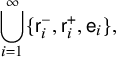
and for
$\Omega \in \mathrm {RESeq}$
 define
$|\Omega |$
define
$|\Omega |$
 to be the number of
$\mathsf {e}_{i}$
to be the number of
$\mathsf {e}_{i}$
 letters in
$\Omega $
letters in
$\Omega $
 . For example,
$\mathsf {r}_{2}^-\mathsf {r}_{3}^+\mathsf {e}_{2}\in \mathrm {RESeq}$
. For example,
$\mathsf {r}_{2}^-\mathsf {r}_{3}^+\mathsf {e}_{2}\in \mathrm {RESeq}$
 and
$|\mathsf {r}_{2}^-\mathsf {r}_{3}^+\mathsf {e}_{2}|=1$
and
$|\mathsf {r}_{2}^-\mathsf {r}_{3}^+\mathsf {e}_{2}|=1$
 . We define a distinguished subset
$\mathrm {RESeq}_n\subset \mathrm {RESeq}$
. We define a distinguished subset
$\mathrm {RESeq}_n\subset \mathrm {RESeq}$
 by
by

Note that every word of
$\mathrm {RESeq}_n$
 begins with
$\mathsf {r}_{1}^-$
begins with
$\mathsf {r}_{1}^-$
 . We will write either
$\Omega _1 \Omega _2$
. We will write either
$\Omega _1 \Omega _2$
 or
$\Omega _1\cdot \Omega _2$
or
$\Omega _1\cdot \Omega _2$
 to describe the concatenation of
$\Omega _1$
to describe the concatenation of
$\Omega _1$
 and
$\Omega _2$
and
$\Omega _2$
 .
.
Definition 4.1. Let
$\operatorname {BNestFor}_n$
 be the quotient of
$\mathrm {RESeq}_n$
be the quotient of
$\mathrm {RESeq}_n$
 by the local relations
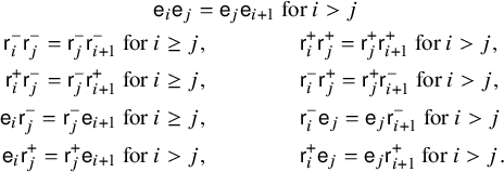
This is well-defined as the relations all preserve
$\mathrm {RESeq}_n$
 .
.
We recall from [Reference Bergeron, Gagnon, Nadeau, Spink and Tewari6, Proposition 9.4] how the equivalence classes in
$\operatorname {BNestFor}_{n}$
 can be represented diagrammatically. A
$\color {blue}{{bicolored\, nested\, forest}}$
can be represented diagrammatically. A
$\color {blue}{{bicolored\, nested\, forest}}$
 is a nested forest in which each internal node has been colored with either black (
 ) or white (
 ). We now define a map from
$\mathrm {RESeq}_{n}$
). We now define a map from
$\mathrm {RESeq}_{n}$
 to bicolored nested forests with support in
$[n]$
to bicolored nested forests with support in
$[n]$
 .
.
Definition 4.2. For
$\Omega \in \mathrm {RESeq}_{n}$
 , the associated bicolored nested forest
$\widehat {F}(\Omega )$
, the associated bicolored nested forest
$\widehat {F}(\Omega )$
 with support in
$[n]$
with support in
$[n]$
 is defined recursively by
$\widehat {F}(\varnothing )=\varnothing $
is defined recursively by
$\widehat {F}(\varnothing )=\varnothing $
 and
and
-
1. $\widehat {F}(\Omega \cdot \mathsf {r}_{i}^-)$
is obtained from
$\widehat {F}(\Omega )$
by inserting a new tree with no internal nodes as a leaf between
$i-1$
and i and relabeling leaves appropriately, -
2. $\widehat {F}(\Omega \cdot \mathsf {r}_{i}^+)$
is obtained from
$\widehat {F}(\Omega )$
by replacing the i-th leaf with a white node
whose children are leaves and relabeling leaves appropriately, and -
3. $\widehat {F}(\Omega \cdot \mathsf {e}_{i})$
is obtained from
$\widehat {F}(\Omega )$
by replacing the i-th leaf with a black node
whose children are leaves and relabeling leaves appropriately.


Example 4.3. We demonstrate the recursive process for
$\Omega =\mathsf {r}_{1}^-\mathsf {r}_{1}^{+}\mathsf {r}_{2}^{-}\mathsf {e}_{1}\mathsf {e}_{3}\mathsf {r}_{2}^+$
 :
:


Theorem 4.4. [Reference Bergeron, Gagnon, Nadeau, Spink and Tewari6, Proposition 9.4]
Two elements
$\Omega ,\ \Omega '\in \mathrm {RESeq}_n$
 are in the same equivalence class of
$\operatorname {BNestFor}_n$
are in the same equivalence class of
$\operatorname {BNestFor}_n$
 if and only if
$\widehat {F}(\Omega )=\widehat {F}(\Omega ')$
if and only if
$\widehat {F}(\Omega )=\widehat {F}(\Omega ')$
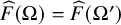 .
.
Going forward, we identify elements of
$\operatorname {BNestFor}_{n}$
 with the associated bicolored nested forest, so that we can write
$\widehat {K} = \widehat {H} \cdot \mathsf {x}_{i}$
with the associated bicolored nested forest, so that we can write
$\widehat {K} = \widehat {H} \cdot \mathsf {x}_{i}$
 to mean
$\widehat {H} = \widehat {F}(\Omega )$
to mean
$\widehat {H} = \widehat {F}(\Omega )$
 and
$\widehat {K} = \widehat {F}(\Omega \cdot \mathsf {x}_{i})$
and
$\widehat {K} = \widehat {F}(\Omega \cdot \mathsf {x}_{i})$
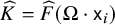 for some
$\Omega \in \mathrm {RESeq}_n$
for some
$\Omega \in \mathrm {RESeq}_n$
 . The defining relations of
$\operatorname {BNestFor}_n$
. The defining relations of
$\operatorname {BNestFor}_n$
 preserve
$|\Omega |$
preserve
$|\Omega |$
 , so it makes sense to discuss
$|\widehat {F}|$
, so it makes sense to discuss
$|\widehat {F}|$
 for
$\widehat {F}\in \operatorname {BNestFor}_{n}$
for
$\widehat {F}\in \operatorname {BNestFor}_{n}$
 . Diagrammatically,
$|\widehat {F}|$
. Diagrammatically,
$|\widehat {F}|$
 is the number of black nodes in
$\widehat {F}$
is the number of black nodes in
$\widehat {F}$
 . See Example 4.3 for a bicolored nested forest built from an
$\Omega \in \mathrm {RESeq}_6$
. See Example 4.3 for a bicolored nested forest built from an
$\Omega \in \mathrm {RESeq}_6$
 with
$|\Omega |=2$
with
$|\Omega |=2$
 .
.
Definition 4.5. We conclude by identifying some distinguished subsets of
$\operatorname {BNestFor}_{n}$
 which will appear in later sections.
-
1. Let $\operatorname {\mathsf {Forest}}_n = \{ \widehat {F} \in \operatorname {BNestFor}_{n} \;|\; \text { each } \Omega \in \widehat {F} \text { has the form }(\mathsf {r}_{1}^{-})^{n-k}\mathsf {e}_{i_1}\cdots \mathsf {e}_{i_k}\}$
; elements of this set map to forests without white nodes in which no nesting occurs, so that the support of each tree is a contiguous interval of
$[n]$
. We will often write
$F\in \operatorname {\mathsf {Forest}}_n$
rather than
$\widehat {F}\in \operatorname {\mathsf {Forest}}_n$
to emphasize the absence of nesting. -
2. Let $\operatorname {Tree}_{n} = \{ \widehat {F} \in \operatorname {BNestFor}_{n} \;|\; |\widehat {F}| = n-1\}$
; elements of this set have representatives of the form
$\mathsf {r}_{1}^- \mathsf {e}_{i_1} \cdots \mathsf {e}_{i_{n-1}}$
and map to singleton trees
$(T_{\mathbf {c}})$
with entirely black nodes.






See the examples given in Figure 3. We note that by definition,
$\operatorname {Tree}_{n} \subseteq \operatorname {\mathsf {Forest}}_n \subseteq \operatorname {BNestFor}_{n}$
 .
.
Examples of Definition 4.5: an element
$T = \mathsf {r}_{1}^-\mathsf {e}_{1}\mathsf {e}_{1}\mathsf {e}_{1}\mathsf {e}_{3} $
 of
$\operatorname {Tree}_{5}$
of
$\operatorname {Tree}_{5}$
 (left) and an element
$F = (\mathsf {r}_{1}^{-})^{3} \mathsf {e}_{1}\mathsf {e}_{4}\mathsf {e}_{5}$
(left) and an element
$F = (\mathsf {r}_{1}^{-})^{3} \mathsf {e}_{1}\mathsf {e}_{4}\mathsf {e}_{5}$
 of
$\operatorname {\mathsf {Forest}}_{6} \setminus \operatorname {Tree}_{6}$
of
$\operatorname {\mathsf {Forest}}_{6} \setminus \operatorname {Tree}_{6}$
 (right).

Figure 3 Long description
The figure consists of two panels.
Left panel: Labeled T equals. It features a horizontal line with five points marked with an x and numbered 1 through 5 from left to right. Above this baseline, a binary tree structure rises. Points 1 and 2 connect to a single node above them. Points 3 and 4 connect to another node above them. The node above 1 and 2 connects to a higher node, which also connects to the node above 3 and 4. Finally, this high node and point 5 connect at the highest peak node of the tree.
Right panel: Labeled F equals. It features a horizontal line with six points marked with an x and numbered 1 through 6 from left to right. This panel shows a forest of two separate trees. The first tree is formed by points 1 and 2 connecting to a single node above. Point 3 remains isolated on the baseline. The second tree starts with points 5 and 6 connecting to a node above them. This node and point 4 then connect to a higher peak node, forming a larger triangular structure.
4.2 Combinatorics of building operations
Lemma 4.6. We have the relations
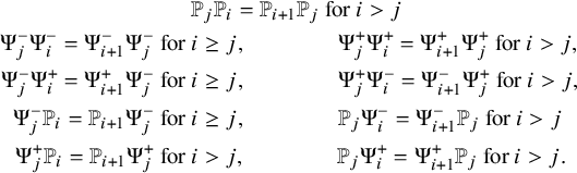
Moreover, these relations hold when all
$\mathbb {P}$
 ’s are replaced by
$\mathbb {G}$
’s are replaced by
$\mathbb {G}$
 ’s.
’s.
Proof. Since
$\mathbb {P}_i=\Psi _i^-\sqcup \mathbb {G}_i\sqcup \Psi _i^+$
 , it suffices to check all of the above relations with
$\mathbb {G}_i$
, it suffices to check all of the above relations with
$\mathbb {G}_i$
 in place of
$\mathbb {P}_i$
in place of
$\mathbb {P}_i$
 . It suffices to show the stronger statement that these relations hold for the operations
$\Psi _i^-$
. It suffices to show the stronger statement that these relations hold for the operations
$\Psi _i^-$
 ,
$\Psi _i^+$
,
$\Psi _i^+$
 , and
$\mathbb {G}_i$
, and
$\mathbb {G}_i$
 on subsets of matrices without considering equivalence classes mod B. These are straightforward so we omit their explicit verification. See Example 4.8 for an illustrative example.
Remark 4.7. The relations in Lemma 4.6 are not exhaustive: in Lemma 8.2 we show that two additional relations are needed to describe all interactions between the building operations.
Example 4.8. The following computation witnesses the relation
$\mathbb {G}_1\mathbb {G}_2=\mathbb {G}_3\mathbb {G}_1$
 :
:
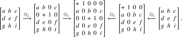
Since the relations of Lemma 4.6 are opposite to the defining relations of
$\operatorname {BNestFor}_n$
 , the following is well-defined.
Definition 4.9. For
$\widehat {F}\in \operatorname {BNestFor}_n$
 , we define
$X(\widehat {F})\subset \mathrm {Fl}_{n}$
, we define
$X(\widehat {F})\subset \mathrm {Fl}_{n}$
 recursively:
$X(\mathsf {r}_{1}^{-})=\mathrm {Fl}_{1}$
recursively:
$X(\mathsf {r}_{1}^{-})=\mathrm {Fl}_{1}$
 is a single point, and
-
1. $X(\widehat {F} \cdot \mathsf {r}_{j}^\pm )=\Psi _{j}^{\pm }X(\widehat {F} )$
-
2. $X(\widehat {F}\cdot \mathsf {e}_{j})=\mathbb P_jX(\widehat {F})$
.


Similarly, we define
$X^{\circ }(\widehat {F})\subset \mathrm {Fl}_{n}$
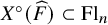 recursively:
$X^{\circ }(\mathsf {r}_{1}^{-})=\mathrm {Fl}_{1}$
recursively:
$X^{\circ }(\mathsf {r}_{1}^{-})=\mathrm {Fl}_{1}$
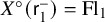 is a single point, and
-
1. $X^{\circ }(\widehat {F}\cdot \mathsf {r}_{j}^{\pm })=\Psi _j^{\pm }X^{\circ }(\widehat {F})$
-
2. $X^{\circ }(\widehat {F}\cdot \mathsf {e}_{j})=\mathbb G_jX^{\circ }(\widehat {F})$
.


In the next section, we will show that
$X^{\circ }(F)$
 is a T-orbit, whose closure is
$X(F)$
is a T-orbit, whose closure is
$X(F)$
 .
.
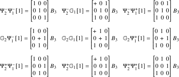
Example 4.10. If
$\widehat {F}=\widehat {F}(\mathsf {r}_{1}^{-}\mathsf {e}_{1}\mathsf {e}_{2})$
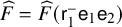 then
$X(\widehat {F})=\mathbb {P}_2\mathbb {P}_1[1]$
then
$X(\widehat {F})=\mathbb {P}_2\mathbb {P}_1[1]$
 is the union of
$9$
is the union of
$9$
 subsets of
$\mathrm {Fl}_{3}$
subsets of
$\mathrm {Fl}_{3}$
 depicted below, with each
$+ \in \mathbb C^{*}$
depicted below, with each
$+ \in \mathbb C^{*}$
 . The T-orbit
$X^{\circ }(\widehat {F})=\mathbb {G}_2\mathbb {G}_1[1]$
. The T-orbit
$X^{\circ }(\widehat {F})=\mathbb {G}_2\mathbb {G}_1[1]$
 appears in the second row and column.
Remark 4.11. We conclude by revisiting the distinguished families from Definition 4.5.
-
1. In Theorem 7.1, we show that the $X(F)$
for
$F \in \operatorname {\mathsf {Forest}}_n$
are the
$\color {blue}{{quasisymmetric\, Schubert\, cycles}}$
of [Reference Nadeau, Spink and Tewari38, Definition 6.2]. -
2. For $T \in \operatorname {Tree}_{n}$
, the
$X(T)$
are the top-dimensional quasisymmetric Schubert cycles, which we use to construct
$\mathrm {QFl}_{n}$
.





5 The Bott manifolds
$X(\widehat {F})$

We now describe the toric structure of varieties
$X(\widehat {F})$
 and
$X^{\circ }(\widehat {F})$
and
$X^{\circ }(\widehat {F})$
 in Definition 4.9.
Theorem 5.1. For
$\widehat {F} \in \operatorname {BNestFor}_{m}$
 , the variety
$X^{\circ }(\widehat {F})$
, the variety
$X^{\circ }(\widehat {F})$
 is a torus orbit in
$\mathrm {Fl}_{m}$
is a torus orbit in
$\mathrm {Fl}_{m}$
 of dimension
$|\widehat {F}|$
of dimension
$|\widehat {F}|$
 . Furthermore,
$X(\widehat {F})$
. Furthermore,
$X(\widehat {F})$
 is the closure of the torus orbit
$X^{\circ }(\widehat {F})$
is the closure of the torus orbit
$X^{\circ }(\widehat {F})$
 in
$\mathrm {Fl}_{m}$
in
$\mathrm {Fl}_{m}$
 .
.
We prove the theorem using the following. Recall the meaning of
$\mathrm {Fl}_{m-1}^{\gamma _i}$
 from Definition 3.2.
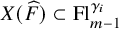
Proposition 5.2. Fix
$\widehat {F}\in \operatorname {BNestFor}_{m-1}$
 , and consider
$X(\widehat {F})\subset \mathrm {Fl}_{m-1}^{\gamma _i}$
, and consider
$X(\widehat {F})\subset \mathrm {Fl}_{m-1}^{\gamma _i}$
 for some fixed
$1\le i \le m$
for some fixed
$1\le i \le m$
 .
.
-
(1) The map $\Psi _i^{-}:X(\widehat {F})\to X(\widehat {F}\cdot \mathsf {r}_{i}^{-})$
is a
$T_m$
-equivariant isomorphism. -
(2) If $i < m$
, the map
$\Psi _i^{+}:X(\widehat {F})\to X(\widehat {F} \cdot \mathsf {r}_{i}^{+})$
is a
$T_m$
-equivariant isomorphism. -
(3) If $i < m$
, there exists a
$T_m$
-equivariant isomorphism
$X(\widehat {F}\cdot \mathsf {e}_{i})\cong \mathsf {Proj}(\mathcal {F}_i/\mathcal {F}_{i-1}\oplus \mathbb {C}_{\chi _i})_{X(\widehat {F})}$
. Furthermore,
$X(\widehat {F}\cdot \mathsf {r}_{i}^-)$
and
$X(\widehat {F}\cdot \mathsf {r}_{i}^+)$
are the
$T_m$
-equivariant sections
$\mathsf {Proj}(\{0\}\oplus \mathbb {C}_{\chi _i})_{X(\widehat {F})}$
and
$\mathsf {Proj}((\mathcal {F}_i/\mathcal {F}_{i-1})\oplus \{0\})_{X(\widehat {F})}$
, respectively.











Proof of Theorem 5.1
The dimension statement follows because each
$\mathbb {G}_i$
 defining
$X^{\circ }(\widehat {F})$
defining
$X^{\circ }(\widehat {F})$
 increases the dimension by
$1$
increases the dimension by
$1$
 and each
$\Psi _i^{\pm }$
and each
$\Psi _i^{\pm }$
 preserves the dimension. To show that
$X^{\circ }(\widehat {F})$
preserves the dimension. To show that
$X^{\circ }(\widehat {F})$
 is a torus orbit, we induct on m. By Proposition 5.2(1) and (2), if we know
$X^{\circ }(\widehat {F})$
is a torus orbit, we induct on m. By Proposition 5.2(1) and (2), if we know
$X^{\circ }(\widehat {F})$
 is a torus orbit, then so is
$X^{\circ }(\widehat {F}\cdot \mathsf {r}_{i}^{\pm })$
is a torus orbit, then so is
$X^{\circ }(\widehat {F}\cdot \mathsf {r}_{i}^{\pm })$
 . Proposition 5.2 further implies that for any
$Y\subset X(\widehat {F})$
. Proposition 5.2 further implies that for any
$Y\subset X(\widehat {F})$
 we have that
$\mathbb {G}_iY\to Y$
we have that
$\mathbb {G}_iY\to Y$
 is a
$\mathbb {C}^*$
is a
$\mathbb {C}^*$
 -bundle obtained from
$\mathbb {P}_iY$
-bundle obtained from
$\mathbb {P}_iY$
 by removing the two distinguished sections. By applying this for
$Y=X^{\circ }(\widehat {F})$
by removing the two distinguished sections. By applying this for
$Y=X^{\circ }(\widehat {F})$
 we conclude that
$T_m$
we conclude that
$T_m$
 acts transitively on
$\mathbb {G}_iX^{\circ }(\widehat {F})=X^{\circ }(\widehat {F}\cdot \mathsf {e}_{i})$
acts transitively on
$\mathbb {G}_iX^{\circ }(\widehat {F})=X^{\circ }(\widehat {F}\cdot \mathsf {e}_{i})$
 from the fact that
$T_m\cong \gamma _i(T_m)\times \mathbb {C}^*_{\chi _i}$
from the fact that
$T_m\cong \gamma _i(T_m)\times \mathbb {C}^*_{\chi _i}$
 with
$\gamma _i(T_m)$
with
$\gamma _i(T_m)$
 acting transitively on the base of the
$\mathbb {C}^*$
acting transitively on the base of the
$\mathbb {C}^*$
 -bundle
$X^{\circ }(\widehat {F}\cdot \mathsf {e}_{i})\to X^{\circ }(\widehat {F})$
-bundle
$X^{\circ }(\widehat {F}\cdot \mathsf {e}_{i})\to X^{\circ }(\widehat {F})$
 and
$\mathbb {C}^*_{\chi _i}$
and
$\mathbb {C}^*_{\chi _i}$
 acting transitively on the fibers while fixing the base. Finally, for any
$Z\subset \mathrm {Fl}_{m-1}$
acting transitively on the fibers while fixing the base. Finally, for any
$Z\subset \mathrm {Fl}_{m-1}$
 we have
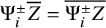
$\Psi _i^{\pm }\overline {Z}=\overline {\Psi _i^{\pm }Z}$
we have
$\Psi _i^{\pm }\overline {Z}=\overline {\Psi _i^{\pm }Z}$
 and
$\mathbb {P}_i\overline {Z}=\overline {\mathbb {P}_iZ}=\overline {\mathbb {G}Z}$
and
$\mathbb {P}_i\overline {Z}=\overline {\mathbb {P}_iZ}=\overline {\mathbb {G}Z}$
 , which shows by induction that
$X(\widehat {F})$
, which shows by induction that
$X(\widehat {F})$
 is the closure of
$X^{\circ }(\widehat {F})$
is the closure of
$X^{\circ }(\widehat {F})$
 .
.
Recall that a
$\color {blue}{{combinatorial\, cube}}$
 is a polytope whose face lattice is identical to that of a cube of the same dimension. If we have a sequence of varieties
$X_1, X_2, \ldots , X_m$
is a polytope whose face lattice is identical to that of a cube of the same dimension. If we have a sequence of varieties
$X_1, X_2, \ldots , X_m$
 where
$X_1=\{\operatorname {pt}\}$
where
$X_1=\{\operatorname {pt}\}$
 is a single point and
$X_i=\mathsf {Proj}(\mathcal {L}_{i-1}\oplus \mathbb {C})_{X_{i-1}}$
is a single point and
$X_i=\mathsf {Proj}(\mathcal {L}_{i-1}\oplus \mathbb {C})_{X_{i-1}}$
 for a toric line bundle
$\mathcal {L}_{i-1}$
for a toric line bundle
$\mathcal {L}_{i-1}$
 on
$X_{i-1}$
on
$X_{i-1}$
 , then
$X_m$
, then
$X_m$
 is a smooth projective toric variety whose moment polytope is a combinatorial cube. The toric structure is defined recursively by saying that if
$T_{i-1}$
is a smooth projective toric variety whose moment polytope is a combinatorial cube. The toric structure is defined recursively by saying that if
$T_{i-1}$
 is the torus for
$X_{i-1}$
is the torus for
$X_{i-1}$
 , then
$X_i$
, then
$X_i$
 is a toric variety for
$T_i:= T_{i-1}\times \mathbb {C}^*$
is a toric variety for
$T_i:= T_{i-1}\times \mathbb {C}^*$
 where
$T_{i-1}$
where
$T_{i-1}$
 acts trivially on the factor of
$\mathbb {C}$
acts trivially on the factor of
$\mathbb {C}$
 and
$\mathbb {C}^*$
and
$\mathbb {C}^*$
 acts by scaling this
$\mathbb {C}$
acts by scaling this
$\mathbb {C}$
 factor. The dense torus orbit can also be obtained by taking
$\mathsf {Proj}(\mathcal {L}_{i-1}\oplus \mathbb {C})_{T_i}$
factor. The dense torus orbit can also be obtained by taking
$\mathsf {Proj}(\mathcal {L}_{i-1}\oplus \mathbb {C})_{T_i}$
 and removing the two distinguished sections. Such an
$X_m$
and removing the two distinguished sections. Such an
$X_m$
 obtained in this way is called a
$\color {blue}{{Bott\, manifold}}$
obtained in this way is called a
$\color {blue}{{Bott\, manifold}}$
 (see [Reference Masuda and Panov37]).
Definition 5.3. For
$\Omega _1,\Omega _2\in \mathrm {RESeq}_n$
 , we say
$\Omega _1\le _{re} \Omega _2$
, we say
$\Omega _1\le _{re} \Omega _2$
 if
$\Omega _1$
if
$\Omega _1$
 is obtained from
$\Omega _2$
is obtained from
$\Omega _2$
 by switching some letters
$\mathsf {e}_{i}$
by switching some letters
$\mathsf {e}_{i}$
 to
$\mathsf {r}_{i}^{\pm }$
to
$\mathsf {r}_{i}^{\pm }$
 .
.
Proposition 5.4. For
$\Omega _{1} \mathsf {e}_{i} \Omega _{2} \in \mathrm {RESeq}_{n}$
 ,
,
-
(1) $\widehat {F}(\Omega _1\mathsf {r}_{i}^+\Omega _2)$
is obtained from
$\widehat {F}(\Omega _1\mathsf {e}_{i}\Omega _2)$
by changing the black node associated to
$\mathsf {e}_{i}$
to a white node, and -
(2) $\widehat {F}(\Omega _1\mathsf {r}_{i}^-\Omega _2)$
is obtained from
$\widehat {F}(\Omega _1\mathsf {e}_{i}\Omega _2)$
by deleting the left edge of the black node associated to
$\mathsf {e}_{i}$
and contracting the resulting node.


In particular, the relation
$\le _{re}$
 descends to a partial order on
$\operatorname {BNestFor}_n$
descends to a partial order on
$\operatorname {BNestFor}_n$
 .
.
Proof. This follows immediately from the way that bicolored nested forests are created recursively from sequences in
$\mathrm {RESeq}_n$
 .
.
We define the operation of
$\color {blue}{{left\, edge\, deletion}}$
 at a node in
$\operatorname {IN}(\widehat {F})$
at a node in
$\operatorname {IN}(\widehat {F})$
 to be the operation described in Proposition 5.4(2). We sometimes emphasize that a forest is obtained by left edge deletion at v by drawing the contracted edge through the former location of v, as shown below.
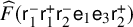
Example 5.5. We demonstrate Proposition 5.4 using the nested forest
$\widehat {F}(\mathsf {r}_{1}^-\mathsf {r}_{1}^{+}\mathsf {r}_{2}^{-}\mathsf {e}_{1}\mathsf {e}_{3}\mathsf {r}_{2}^+)$
 from Example 4.3. Three examples of
$\le _{re}$
from Example 4.3. Three examples of
$\le _{re}$
 -smaller nested forests are:

Definition 5.6. For
$\widehat {F}\in \operatorname {BNestFor}_n$
 , we define

Restricting
$\le _{re}$
 to
$\mathrm {Face}(\widehat {F})$
to
$\mathrm {Face}(\widehat {F})$
 gives the face poset of a
$|\widehat {F}|$
gives the face poset of a
$|\widehat {F}|$
 -dimensional cube. Indeed, the choice of whether to change each black node white or to perform left edge deletion is equivalent to choosing one from a pair of opposite faces. Figure 6 shows in the left panel two such cubes and the elements of
$\mathrm {Face}(\widehat {F})$
-dimensional cube. Indeed, the choice of whether to change each black node white or to perform left edge deletion is equivalent to choosing one from a pair of opposite faces. Figure 6 shows in the left panel two such cubes and the elements of
$\mathrm {Face}(\widehat {F})$
 associated with each face. We now give this interpretation a geometric meaning.
Theorem 5.7. For
$\widehat {F}\in \operatorname {BNestFor}_n$
 ,
$X(\widehat {F})\subset \mathrm {Fl}_{n}$
,
$X(\widehat {F})\subset \mathrm {Fl}_{n}$
 is a Bott manifold of dimension
$|\widehat {F}|$
is a Bott manifold of dimension
$|\widehat {F}|$
 with dense torus orbit
$X^{\circ }(\widehat {F})$
with dense torus orbit
$X^{\circ }(\widehat {F})$
 . The distinct torus orbits of
$X(\widehat {F})$
. The distinct torus orbits of
$X(\widehat {F})$
 are given by
$\{X^{\circ }(\widehat {G}):\widehat {G}\in \mathrm {Face}(\widehat {F})\}$
are given by
$\{X^{\circ }(\widehat {G}):\widehat {G}\in \mathrm {Face}(\widehat {F})\}$
 , and the distinct torus orbit closures are given by
$\{X(\widehat {G}):\widehat {G}\in \mathrm {Face}(\widehat {F})\}$
, and the distinct torus orbit closures are given by
$\{X(\widehat {G}):\widehat {G}\in \mathrm {Face}(\widehat {F})\}$
 .
.
Proof. By Proposition 5.2, any
$\Omega \in \mathrm {RESeq}_n$
 representing
$\widehat {F}$
representing
$\widehat {F}$
 induces a Bott manifold structure on
$X(\widehat {F})$
induces a Bott manifold structure on
$X(\widehat {F})$
 with dense torus orbit
$X^{\circ }(\widehat {F})$
with dense torus orbit
$X^{\circ }(\widehat {F})$
 as described above, and the dimension is
$|\widehat {F}|$
as described above, and the dimension is
$|\widehat {F}|$
 by Theorem 5.1.
Since Theorem 5.1 shows that the closure of the torus orbit
$X^{\circ }(\widehat {G})$
 is
$X(\widehat {G})$
is
$X(\widehat {G})$
 , it remains to describe the distinct torus-orbit closures. We proceed inductively. Suppose the result holds for all
$\widehat {F}\in \operatorname {BNestFor}_{n-1}$
, it remains to describe the distinct torus-orbit closures. We proceed inductively. Suppose the result holds for all
$\widehat {F}\in \operatorname {BNestFor}_{n-1}$
 ; we aim to prove it for each
$\widehat {F}\cdot \mathsf {x}_{i}\in \operatorname {BNestFor}_n$
; we aim to prove it for each
$\widehat {F}\cdot \mathsf {x}_{i}\in \operatorname {BNestFor}_n$
 .
.
First, note that
$\Psi _i^{\pm }:X(\widehat {F})\to X(\widehat {F}\cdot \mathsf {r}_{i}^{\pm })$
 is an isomorphism and moreover induces a bijection between torus orbit closures via

so we conclude the result for
$\widehat {F}\cdot \mathsf {r}_{i}^{\pm }$
 as
$\mathrm {Face}(\widehat {F}\cdot \mathsf {r}_{i}^{\pm })=\{\widehat {G}\cdot \mathsf {r}_{i}^{\pm }:\widehat {G}\in \mathrm {Face}(\widehat {F})\}$
as
$\mathrm {Face}(\widehat {F}\cdot \mathsf {r}_{i}^{\pm })=\{\widehat {G}\cdot \mathsf {r}_{i}^{\pm }:\widehat {G}\in \mathrm {Face}(\widehat {F})\}$
 . Consider now the
$\mathbb {P}^1$
. Consider now the
$\mathbb {P}^1$
 -bundle
$X(\widehat {F}\cdot \mathsf {e}_{i})\to X(\widehat {F})$
-bundle
$X(\widehat {F}\cdot \mathsf {e}_{i})\to X(\widehat {F})$
 . For any projective toric variety X with a toric line bundle
$\mathcal {L}$
. For any projective toric variety X with a toric line bundle
$\mathcal {L}$
 , the torus orbit closures on the toric variety
$\mathsf {Proj}(\mathcal {L}\oplus \mathbb {C})$
, the torus orbit closures on the toric variety
$\mathsf {Proj}(\mathcal {L}\oplus \mathbb {C})$
 are given by the
$\mathbb {P}^1$
are given by the
$\mathbb {P}^1$
 -bundles over the torus orbit closures in X, together with the images of the torus orbit closures in X in the two disjoint sections of the split projective bundle. Consequently by Proposition 5.2 the torus orbit closures in
$X(\widehat {F})$
-bundles over the torus orbit closures in X, together with the images of the torus orbit closures in X in the two disjoint sections of the split projective bundle. Consequently by Proposition 5.2 the torus orbit closures in
$X(\widehat {F})$
 are given by

and we conclude as
$\mathrm {Face}(\widehat {F}\cdot \mathsf {e}_{i})=\bigcup _{\widehat {G}\in \mathrm {Face}(\widehat {F})}\{\widehat {G}\cdot \mathsf {r}_{i}^-,\widehat {G}\cdot \mathsf {r}_{i}^+,\widehat {G}\cdot \mathsf {e}_{i}\}$
 .
.
6 Torus fixed points of
$X(\widehat {F})$

In this section, we describe the combinatorics of the fixed point sets

As the following theorem shows, elements of
$I_{\widehat {F}}$
 always lie in
$\operatorname {NC}_n$
always lie in
$\operatorname {NC}_n$
 .
.
Theorem 6.1. For any
$\widehat {F} \in \operatorname {BNestFor}_{n}$
 , we have

In particular, if
$\widehat {G} \in \operatorname {BNestFor}_{n}$
 has
$|\widehat {G}|=0$
has
$|\widehat {G}|=0$
 , then
$X_{\widehat {G}}=\{\operatorname {NCPerm}(\widehat {G})\}$
, then
$X_{\widehat {G}}=\{\operatorname {NCPerm}(\widehat {G})\}$
 .
.
Example 6.2. We apply the theorem to the fixed point set for the nested forest
$\widehat {F}(\mathsf {r}_{1}^-\mathsf {r}_{1}^{+}\mathsf {r}_{2}^{-}\mathsf {e}_{1}\mathsf {e}_{3}\mathsf {r}_{2}^+)$
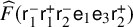 from Examples 4.3 and 5.5. We have:
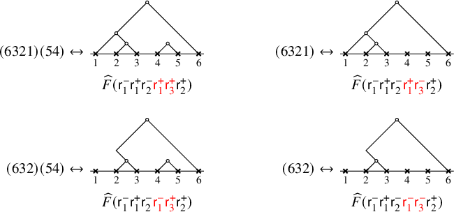
Going forward, we will abuse notation and treat
$\Psi ^{-}_{i}$
 and
$\Psi ^{+}_{i}$
and
$\Psi ^{+}_{i}$
 as maps on permutations rather than just permutation matrices. These are given by the group homomorphism
$\Psi _i^-:S_{n-1}\hookrightarrow S_n$
as maps on permutations rather than just permutation matrices. These are given by the group homomorphism
$\Psi _i^-:S_{n-1}\hookrightarrow S_n$
 , induced by the increasing injection
$\{1,\ldots ,n-1\}\hookrightarrow \{1,\ldots ,i-1,i+1,\ldots ,n\}$
, induced by the increasing injection
$\{1,\ldots ,n-1\}\hookrightarrow \{1,\ldots ,i-1,i+1,\ldots ,n\}$
 onto the subgroup of
$S_n$
onto the subgroup of
$S_n$
 with
$u(i)=i$
with
$u(i)=i$
 , and
$\Psi _i^+w=(\Psi _i^-w)s_i$
, and
$\Psi _i^+w=(\Psi _i^-w)s_i$
 .
.
Proof of Theorem 6.1
We know from Theorem 5.7 that the fixed point set
$I_{\widehat {F}}$
 is given by the points
$X_{\widehat {G}}$
is given by the points
$X_{\widehat {G}}$
 such that
$\widehat {G}\in \Vert (\widehat {F})$
such that
$\widehat {G}\in \Vert (\widehat {F})$
 . Therefore we need only verify the statement when
$|\widehat {G}| = 0$
. Therefore we need only verify the statement when
$|\widehat {G}| = 0$
 , meaning that
$\widehat {G}$
, meaning that
$\widehat {G}$
 is represented by a sequence of
$\mathsf {r}_{i}^{\pm }$
is represented by a sequence of
$\mathsf {r}_{i}^{\pm }$
 .
.
For
$n=1$
 we have
$\widehat {G}=\mathsf {r}_{1}^-$
we have
$\widehat {G}=\mathsf {r}_{1}^-$
 and
$X_{\widehat {G}} = \{\operatorname {id}_{S_1}\} = \{\operatorname {NCPerm}(\widehat {G})\}$
and
$X_{\widehat {G}} = \{\operatorname {id}_{S_1}\} = \{\operatorname {NCPerm}(\widehat {G})\}$
 . For
$n>1$
. For
$n>1$
 , by the recursive construction of
$X_{\widehat {G}}$
, by the recursive construction of
$X_{\widehat {G}}$
 in Definition 4.9 it suffices to show that

We check these by comparing the definition of
$\widehat {F}\cdot \mathsf {r}_{i}^{\pm }$
 with that of
$\Psi ^{\pm }_{i}$
with that of
$\Psi ^{\pm }_{i}$
 : the former is straightforward, and the latter follows from the fact that for a backwards cycle C on a set A containing i but not
$i+1$
: the former is straightforward, and the latter follows from the fact that for a backwards cycle C on a set A containing i but not
$i+1$
 , the product
$C(i\;i+1)$
, the product
$C(i\;i+1)$
 is the backwards cycle on
$A\sqcup \{i+1\}$
is the backwards cycle on
$A\sqcup \{i+1\}$
 .
.
We now characterize
$I_{\widehat {F}}$
 in a manner that connects nested forests to factorizations of noncrossing partitions, as mentioned in Remark 2.2. For each internal node
$v \in \operatorname {IN}(\widehat {F})$
in a manner that connects nested forests to factorizations of noncrossing partitions, as mentioned in Remark 2.2. For each internal node
$v \in \operatorname {IN}(\widehat {F})$
 , let
$\tau _{v}$
, let
$\tau _{v}$
 denote the transposition
$(i\, j)$
denote the transposition
$(i\, j)$
 of the rightmost leaf descendant i of
$v_{L}$
of the rightmost leaf descendant i of
$v_{L}$
 and the rightmost leaf descendant j of v, as shown in Figure 4.
A bicolored nested forest with internal nodes labeled by transpositions
$\tau _v$
 .
.
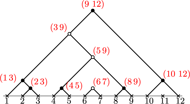
Figure 4 Long description
The diagram consists of a tree structure with nodes connected by diagonal lines. The root node at the top is a solid black circle labeled with the red transposition (9 12). From this root, two branches descend. The right branch leads directly to a solid black node labeled (10 12), which then splits to leaf positions 10 and 12. The left branch leads to an open white node labeled (3 9). From (3 9), the left branch descends to a solid black node labeled (1 3), which splits to leaf positions 1 and 3, with a further sub-node (2 3) splitting to leaf positions 2 and 3. The right branch from (3 9) leads to an open white node labeled (5 9). From (5 9), the left branch leads to a solid black node (4 5) splitting to leaf positions 4 and 5. The right branch from (5 9) leads to a solid black node (8 9) splitting to leaf positions 8 and 9. Between these branches, an isolated open white node (6 7) splits to leaf positions 6 and 7. The baseline is a horizontal line marked with ‘x’ symbols and numbered 1 through 12 from left to right.
Say that a total order on
$\operatorname {IN}(\widehat {F})$
 is a
$\color {blue}{{linear\, extension}}$
is a
$\color {blue}{{linear\, extension}}$
 of
$\widehat {F}$
of
$\widehat {F}$
 if each
$v \in \operatorname {IN}(\widehat {F})$
if each
$v \in \operatorname {IN}(\widehat {F})$
 is preceded by all of its ancestors. As we now explain, the
$\tau _{v}$
is preceded by all of its ancestors. As we now explain, the
$\tau _{v}$
 have the property that any two product orders on

which are linear extensions of
$\widehat {F}$
 are related entirely by commuting factors past one another. Indeed, any two linear extensions are related by repeatedly swapping adjacent elements
$v,v'$
are related entirely by commuting factors past one another. Indeed, any two linear extensions are related by repeatedly swapping adjacent elements
$v,v'$
 which are not ancestor and descendant, and for such a pair the transpositions
$\tau _v=(i,j)$
which are not ancestor and descendant, and for such a pair the transpositions
$\tau _v=(i,j)$
 and
$\tau _{v'}=(k,\ell )$
and
$\tau _{v'}=(k,\ell )$
 are disjoint and hence commute.
Thus (6.2) is unambiguously defined as the product of the vertices of
$\widehat {F}$
 taken in any order dictated by a linear extension of
$\widehat {F}$
taken in any order dictated by a linear extension of
$\widehat {F}$
 . For the same reasons, one can define the product
$\prod _{v \in S} \tau _{v}$
. For the same reasons, one can define the product
$\prod _{v \in S} \tau _{v}$
 for any
$S\subset \operatorname {IN}(\widehat {F})$
for any
$S\subset \operatorname {IN}(\widehat {F})$
 .
.
Theorem 6.3. For each
$\widehat {F} \in \operatorname {BNestFor}_{n}$
 , we have

In particular,
$\operatorname {NCPerm}(\widehat {F}) = \prod _{v \in \operatorname {IN}(\widehat {F})} \tau _{v}$
 .
.
Proof. We first show the claim holds when
$\widehat {F}$
 has only white nodes, so that
$I_{\widehat {F}} = \{\operatorname {NCPerm}(\widehat {F})\}$
has only white nodes, so that
$I_{\widehat {F}} = \{\operatorname {NCPerm}(\widehat {F})\}$
 by Theorem 6.1 and the claim amounts to
$\operatorname {NCPerm}(\widehat {F}) = \prod _{v\in \operatorname {IN}(\widehat {F})}\tau _v$
by Theorem 6.1 and the claim amounts to
$\operatorname {NCPerm}(\widehat {F}) = \prod _{v\in \operatorname {IN}(\widehat {F})}\tau _v$
 . We proceed by induction on
$|\operatorname {IN}(\widehat {F})|$
. We proceed by induction on
$|\operatorname {IN}(\widehat {F})|$
 . If
$\widehat {F}$
. If
$\widehat {F}$
 has no nodes, then the claim holds trivially. Otherwise let
$v_{0}$
has no nodes, then the claim holds trivially. Otherwise let
$v_{0}$
 be the root of a tree in
$\widehat {F}$
be the root of a tree in
$\widehat {F}$
 that is not nested under any other tree, so that
$v_{0}$
that is not nested under any other tree, so that
$v_{0}$
 is the first element in some linear extension of
$\widehat {F}$
is the first element in some linear extension of
$\widehat {F}$
 . Let
$\widehat {G}$
. Let
$\widehat {G}$
 be the forest obtained by deleting
$v_{0}$
be the forest obtained by deleting
$v_{0}$
 and all incident edges. As
$|\operatorname {IN}(\widehat {G})| < |\operatorname {IN}(\widehat {F})|$
and all incident edges. As
$|\operatorname {IN}(\widehat {G})| < |\operatorname {IN}(\widehat {F})|$
 , our inductive hypothesis guarantees that
$\operatorname {NCPerm}(\widehat {G}) = \prod _{v \in \operatorname {IN}(\widehat {G})} \tau _{v}$
, our inductive hypothesis guarantees that
$\operatorname {NCPerm}(\widehat {G}) = \prod _{v \in \operatorname {IN}(\widehat {G})} \tau _{v}$
 is the unique element of
$I_{\widehat {G}}$
is the unique element of
$I_{\widehat {G}}$
 . Moreover,
$\operatorname {NCPerm}(\widehat {G}) = \prod _{v \in \operatorname {IN}(\widehat {F})-\{v_0\}} \tau _{v}$
. Moreover,
$\operatorname {NCPerm}(\widehat {G}) = \prod _{v \in \operatorname {IN}(\widehat {F})-\{v_0\}} \tau _{v}$
 , since for
$v \in \operatorname {IN}(\widehat {G})$
, since for
$v \in \operatorname {IN}(\widehat {G})$
 the value of
$\tau _v$
the value of
$\tau _v$
 does not depend on whether we consider v as a node of
$\widehat {F}$
does not depend on whether we consider v as a node of
$\widehat {F}$
 or
$\widehat {G}$
or
$\widehat {G}$
 . It therefore suffices to show that
$\tau _{v_0}\operatorname {NCPerm}(\widehat {F})=\operatorname {NCPerm}(\widehat {G})$
. It therefore suffices to show that
$\tau _{v_0}\operatorname {NCPerm}(\widehat {F})=\operatorname {NCPerm}(\widehat {G})$
 , which follows from the fact that if
$c_A$
, which follows from the fact that if
$c_A$
 and
$c_B$
and
$c_B$
 are backwards cycles with
$\max A<\min B$
are backwards cycles with
$\max A<\min B$
 , then
$(\max A, \max B)c_Ac_B=c_{A\sqcup B}$
, then
$(\max A, \max B)c_Ac_B=c_{A\sqcup B}$
 .
.
We now consider the general case of
$\widehat {F} \in \operatorname {BNestFor}_{n}$
 . By Theorem 6.1, we have that
$I_{\widehat {F}} = \{ \operatorname {NCPerm}(\widehat {G}) \;|\; \widehat {G} \in \Vert (\widehat {F}) \}$
. By Theorem 6.1, we have that
$I_{\widehat {F}} = \{ \operatorname {NCPerm}(\widehat {G}) \;|\; \widehat {G} \in \Vert (\widehat {F}) \}$
 . Further, each
$\widehat {G} \in \Vert (\widehat {F})$
. Further, each
$\widehat {G} \in \Vert (\widehat {F})$
 is obtained precisely by performing left edge deletion at some subset S of black nodes from
$\widehat {F}$
is obtained precisely by performing left edge deletion at some subset S of black nodes from
$\widehat {F}$
 and changing the remaining black nodes to white nodes. Thus applying the special case proved above to each
$\widehat {G} \in \Vert (\widehat {F})$
and changing the remaining black nodes to white nodes. Thus applying the special case proved above to each
$\widehat {G} \in \Vert (\widehat {F})$
 , we see that the theorem holds for
$\widehat {F}$
, we see that the theorem holds for
$\widehat {F}$
 .
.
Recall that the moment polytope for each
$X(\widehat {F})$
 is a combinatorial cube with vertices corresponding to the fixed point set
$I_{\widehat {F}}$
is a combinatorial cube with vertices corresponding to the fixed point set
$I_{\widehat {F}}$
 .
.
Corollary 6.4. For
$\widehat {F} \in \operatorname {BNestFor}_{n}$
 ,
$I_{\widehat {F}}$
,
$I_{\widehat {F}}$
 is an induced Boolean sublattice in the Kreweras order, and
$w \mapsto w \cdot \lambda $
is an induced Boolean sublattice in the Kreweras order, and
$w \mapsto w \cdot \lambda $
 maps
$I_{\widehat {F}}$
maps
$I_{\widehat {F}}$
 onto the vertices of the moment polytope of
$X(\widehat {F})$
onto the vertices of the moment polytope of
$X(\widehat {F})$
 for the dominant weight
$\lambda $
for the dominant weight
$\lambda $
 in such a way that the Hasse diagram of
$I_{\widehat {F}}$
in such a way that the Hasse diagram of
$I_{\widehat {F}}$
 is identified with the
$1$
is identified with the
$1$
 -skeleton of the polytope.
Proof. By Theorem 6.1,
$I_{\widehat {F}} \subseteq \operatorname {NC}_{n}$
 . By [Reference Heller and Schwer30, Lemma 2.11], this is an induced Boolean sublattice of the Kreweras order. Moreover, using the description of
$I_{\widehat {F}}$
. By [Reference Heller and Schwer30, Lemma 2.11], this is an induced Boolean sublattice of the Kreweras order. Moreover, using the description of
$I_{\widehat {F}}$
 given in Proposition 6.3, the edges of the moment polytope connect exactly those pairs of elements of
$I_{\widehat {F}}$
given in Proposition 6.3, the edges of the moment polytope connect exactly those pairs of elements of
$I_{\widehat {F}}$
 which differ by the inclusion of a single
$\tau _{v}$
which differ by the inclusion of a single
$\tau _{v}$
 .
.
7 Translated Richardsons and polypositroids
In this section we relate our
$X(\widehat {F})$
 to certain Richardson varieties previously studied in [Reference Nadeau, Spink and Tewari39, Reference Nadeau and Tewari40] and the quasisymmetric Schubert cycles of [Reference Nadeau, Spink and Tewari38]; see Remark 7.3. We then use this connection to describe the moment polytope of each
$X(\widehat {F})$
to certain Richardson varieties previously studied in [Reference Nadeau, Spink and Tewari39, Reference Nadeau and Tewari40] and the quasisymmetric Schubert cycles of [Reference Nadeau, Spink and Tewari38]; see Remark 7.3. We then use this connection to describe the moment polytope of each
$X(\widehat {F})$
 as a polypositroid [Reference Lam and Postnikov33].
Recall that a Richardson variety is the intersection
$X^{v}_{w} = X^{v} \cap X_{w}$
 , which is nonempty if and only if
$w \le v$
, which is nonempty if and only if
$w \le v$
 . Recall further that
$\boldsymbol {c}$
. Recall further that
$\boldsymbol {c}$
 denotes the Coxeter element
$s_{n-1}\cdots s_1\in S_n$
denotes the Coxeter element
$s_{n-1}\cdots s_1\in S_n$
 . It is straightforward to see that
$w \le w \boldsymbol {c}$
. It is straightforward to see that
$w \le w \boldsymbol {c}$
 if and only if
$w\in S_{n-1}$
if and only if
$w\in S_{n-1}$
 , and in this case the Richardson variety
$X^{w \boldsymbol {c}}_{w}$
, and in this case the Richardson variety
$X^{w \boldsymbol {c}}_{w}$
 is known to be an
$(n-1)$
is known to be an
$(n-1)$
 -dimensional toric variety [Reference Nadeau, Spink and Tewari38]. Consider now the image of each
$X^{w \boldsymbol {c}}_{w}$
-dimensional toric variety [Reference Nadeau, Spink and Tewari38]. Consider now the image of each
$X^{w \boldsymbol {c}}_{w}$
 under left multiplication by
$w^{-1}$
under left multiplication by
$w^{-1}$
 .
.
Theorem 7.1. We have

In particular, there are
$\operatorname {Cat}_{n-1}$
 distinct translated Richardson varieties, one for each
$T\in \mathrm {Tree}_n$
distinct translated Richardson varieties, one for each
$T\in \mathrm {Tree}_n$
 .
.
For
$T\in \operatorname {Tree}_n$
 recall that we have

for any sequence
$\mathsf {r}_{1}^-\mathsf {e}_{i_{1}}\mathsf {e}_{i_{2}}\cdots \mathsf {e}_{i_{n-1}}$
 associated to T. For any m, let
$\varepsilon _i$
associated to T. For any m, let
$\varepsilon _i$
 be the map from
$S_{m-1}$
be the map from
$S_{m-1}$
 to
$S_m$
to
$S_m$
 that, in one-line notation, inserts a
$1$
that, in one-line notation, inserts a
$1$
 into the i-th position and increases the remaining numbers by
$1$
into the i-th position and increases the remaining numbers by
$1$
 . For example,
$\varepsilon _3 15684237=261795348$
. For example,
$\varepsilon _3 15684237=261795348$
 . Note that this coincides with the map
$\Psi _{1,i}^{-}$
. Note that this coincides with the map
$\Psi _{1,i}^{-}$
 restricted to permutation matrices. However, unlike
$\Psi _{1,i}^-$
restricted to permutation matrices. However, unlike
$\Psi _{1,i}^-$
 , we shall reserve
$\varepsilon _i$
, we shall reserve
$\varepsilon _i$
 for use on permutations only.
Lemma 7.2. Let
$Y(u,v):= u^{-1}X^v_u$
 . Then
$\mathbb {P}_iY(u,v)=Y({\varepsilon _i u},{\varepsilon _{i+1}v}).$
. Then
$\mathbb {P}_iY(u,v)=Y({\varepsilon _i u},{\varepsilon _{i+1}v}).$

Proof. In [Reference Nadeau, Spink and Tewari38, §4] it was shown that
$\pi _i^{-1}\pi _i\Psi _{1,i}X^v_u=X^{\varepsilon _{i+1}v}_{\varepsilon _i u}$
 . Since
$\pi _i$
. Since
$\pi _i$
 is equivariant with respect to left multiplication, we get the following sequence of equalities

where we use the fact that
$(\varepsilon _i u)^{-1}\Psi _{1,i}=\Psi _{i}^- u^{-1}$
 .
.
Proof of Theorem 7.1
Suppose first that
$T\in \mathrm {Tree}_n$
 is associated to the sequence
$\mathsf {r}_{1}^-\mathsf {e}_{i_{1}}\cdots \mathsf {e}_{i_{n-1}}\in \mathrm {RESeq}_n$
is associated to the sequence
$\mathsf {r}_{1}^-\mathsf {e}_{i_{1}}\cdots \mathsf {e}_{i_{n-1}}\in \mathrm {RESeq}_n$
 . Let
$v= \varepsilon _{i_{n-1}+1}\cdots \varepsilon _{i_1+1}\operatorname {id}_{S_1}$
. Let
$v= \varepsilon _{i_{n-1}+1}\cdots \varepsilon _{i_1+1}\operatorname {id}_{S_1}$
 and
$u=\varepsilon _{i_{n-1}}\cdots \varepsilon _{i_1}\operatorname {id}_{S_1}$
and
$u=\varepsilon _{i_{n-1}}\cdots \varepsilon _{i_1}\operatorname {id}_{S_1}$
 . By [Reference Nadeau, Spink and Tewari38, Proposition B.4(2)] we have
$v=u\boldsymbol {c}$
. By [Reference Nadeau, Spink and Tewari38, Proposition B.4(2)] we have
$v=u\boldsymbol {c}$
 and
$u(n)=n$
and
$u(n)=n$
 . By repeated applications of Lemma 7.2 we have
$X(T)=u^{-1}X_u^{v}=u^{-1}X_u^{u\boldsymbol {c}}$
. By repeated applications of Lemma 7.2 we have
$X(T)=u^{-1}X_u^{v}=u^{-1}X_u^{u\boldsymbol {c}}$
 .
.
Conversely given
$u\in S_{n-1}$
 , by induction one can show that
$u=\varepsilon _{i_{n-1}}\cdots \varepsilon _{i_1}\operatorname {id}_{S_1}$
, by induction one can show that
$u=\varepsilon _{i_{n-1}}\cdots \varepsilon _{i_1}\operatorname {id}_{S_1}$
 for some sequence
$i_{1},\ldots ,i_{n-1}$
for some sequence
$i_{1},\ldots ,i_{n-1}$
 with
$i_j\le j$
with
$i_j\le j$
 , and the tree
$T\in \mathrm {Tree}_n$
, and the tree
$T\in \mathrm {Tree}_n$
 associated to the sequence
$\mathsf {r}_{1}^-\mathsf {e}_{i_{1}}\cdots \mathsf {e}_{i_{n-1}}\in \mathrm {RESeq}_n$
associated to the sequence
$\mathsf {r}_{1}^-\mathsf {e}_{i_{1}}\cdots \mathsf {e}_{i_{n-1}}\in \mathrm {RESeq}_n$
 has
$X(T)=u^{-1}X^{u\boldsymbol {c}}_u$
has
$X(T)=u^{-1}X^{u\boldsymbol {c}}_u$
 .
.
Showing that there are
$\operatorname {Cat}_{n-1}$
 -many distinct translated Richardson varieties amounts to showing that the
$X(T)$
-many distinct translated Richardson varieties amounts to showing that the
$X(T)$
 for
$T\in \mathrm {Tree}_n$
for
$T\in \mathrm {Tree}_n$
 are distinct. This follows either from the identification with the quasisymmetric Schubert cycles of [Reference Nadeau, Spink and Tewari38] as described in Remark 7.3; a second proof can be obtained using the results of Section 8: we characterize when two forests in
$\operatorname {BNestFor}_n$
are distinct. This follows either from the identification with the quasisymmetric Schubert cycles of [Reference Nadeau, Spink and Tewari38] as described in Remark 7.3; a second proof can be obtained using the results of Section 8: we characterize when two forests in
$\operatorname {BNestFor}_n$
 produce the same torus-orbit closure, and in particular show that this does not occur for any two trees.
Remark 7.3. In [Reference Nadeau, Spink and Tewari38] certain translates
$u^{-1}X^v_u$
 of Richardson varieties called
$\color {blue}{{quasisymmetric}} \color {blue}{{Schubert\, cycles}}$
of Richardson varieties called
$\color {blue}{{quasisymmetric}} \color {blue}{{Schubert\, cycles}}$
 were defined for any forest
$F\in \operatorname {\mathsf {Forest}}_n$
were defined for any forest
$F\in \operatorname {\mathsf {Forest}}_n$
 . The description of
$X(T)$
. The description of
$X(T)$
 for
$T=\mathsf {r}_{1}^-\mathsf {e}_{i_1}\cdots \mathsf {e}_{i_{n-1}}\in \mathrm {Tree}_{n}$
for
$T=\mathsf {r}_{1}^-\mathsf {e}_{i_1}\cdots \mathsf {e}_{i_{n-1}}\in \mathrm {Tree}_{n}$
 as a translated Richardson variety is exactly the same as the description of the quasisymmetric Schubert cycle associated to T in [Reference Nadeau, Spink and Tewari38] (matching the notation, T would have been described as associated to a sequence
$\mathsf {r}_{1}\mathsf {t}_{i_1}\cdots \mathsf {t}_{i_{n-1}}\in \mathrm {RTSeq}_n$
as a translated Richardson variety is exactly the same as the description of the quasisymmetric Schubert cycle associated to T in [Reference Nadeau, Spink and Tewari38] (matching the notation, T would have been described as associated to a sequence
$\mathsf {r}_{1}\mathsf {t}_{i_1}\cdots \mathsf {t}_{i_{n-1}}\in \mathrm {RTSeq}_n$
 ). More generally for
$F\in \operatorname {\mathsf {Forest}}_n$
). More generally for
$F\in \operatorname {\mathsf {Forest}}_n$
 , applying Lemma 7.2 recursively to
$X((\mathsf {r}_{1}^-)^{n-k})=X^{\operatorname {id}_{S_{n-k}}}_{\operatorname {id}_{S_{n-k}}}\subset \mathrm {Fl}_{n-k}$
, applying Lemma 7.2 recursively to
$X((\mathsf {r}_{1}^-)^{n-k})=X^{\operatorname {id}_{S_{n-k}}}_{\operatorname {id}_{S_{n-k}}}\subset \mathrm {Fl}_{n-k}$
 realizes each
$X(F)$
realizes each
$X(F)$
 as the quasisymmetric Schubert cycle associated to F.
Recall that for a Richardson variety
$X^v_u$
 , the moment polytope is the
$\color {blue}{{twisted\ Bruhat\ interval}} \color {blue}{{polytope}}$
, the moment polytope is the
$\color {blue}{{twisted\ Bruhat\ interval}} \color {blue}{{polytope}}$
 defined by

Faces of twisted Bruhat interval polytopes are themselves twisted Bruhat interval polytopes [Reference Tsukerman and Williams44, Theorem 7.13]. Since the torus orbit closures in a fixed toric Richardson variety correspond to faces of the associated Bruhat interval polytope, we infer that every torus orbit closure in a toric Richardson variety is also a toric Richardson variety (see also [Reference Tsukerman and Williams44, Proposition 7.12]). This yields the following corollary.
Corollary 7.4. Every
$X(\widehat {F})$
 is the left-translate of a toric Richardson variety by an element of
$S_n$
is the left-translate of a toric Richardson variety by an element of
$S_n$
 .
.
Remark 7.5. Theorem 7.1 provides an alternate perspective on the presence of noncrossing partitions arising as torus fixed points of
$X(\widehat {F})$
 . Indeed, consider a fixed point
$u \in I_{T}$
. Indeed, consider a fixed point
$u \in I_{T}$
 for
$T \in \mathrm {Tree}_{n}$
for
$T \in \mathrm {Tree}_{n}$
 . Using the fact that
$X(T)$
. Using the fact that
$X(T)$
 is a translated Richardson variety we will show that
$u \in \operatorname {NC}_{n}$
is a translated Richardson variety we will show that
$u \in \operatorname {NC}_{n}$
 . To begin, choose a maximal chain from w to
$w\boldsymbol {c}$
. To begin, choose a maximal chain from w to
$w\boldsymbol {c}$
 containing
$wu$
containing
$wu$
 in the Bruhat order. Left translation by
$w^{-1}$
in the Bruhat order. Left translation by
$w^{-1}$
 gives a factorization of
$\boldsymbol {c}$
gives a factorization of
$\boldsymbol {c}$
 as a product of transpositions
$\tau _1\cdots \tau _{n-1}$
as a product of transpositions
$\tau _1\cdots \tau _{n-1}$
 with
$u=\tau _1\cdots \tau _{m}$
with
$u=\tau _1\cdots \tau _{m}$
 for
$m=\ell (u)-\ell (w)$
for
$m=\ell (u)-\ell (w)$
 . Hence
$u\in \operatorname {NC}_n$
. Hence
$u\in \operatorname {NC}_n$
 by the characterization of
$\operatorname {NC}_{n}$
by the characterization of
$\operatorname {NC}_{n}$
 due to Biane [Reference Biane9].
The description of
$X(T)$
 for
$T\in \mathrm {Tree}_{n}$
for
$T\in \mathrm {Tree}_{n}$
 as a translated Richardson variety
$w^{-1}X^{wc}_w$
as a translated Richardson variety
$w^{-1}X^{wc}_w$
 implies that its moment polytope is
$w^{-1}Q^{wc}_w$
implies that its moment polytope is
$w^{-1}Q^{wc}_w$
 , and this leads to a description of the defining hyperplanes for the moment polytope. Recall the canonical labelling of T given in Section 2.3 and suppose that i is the label of an internal node. Let
$\operatorname {Right}(T,i)$
, and this leads to a description of the defining hyperplanes for the moment polytope. Recall the canonical labelling of T given in Section 2.3 and suppose that i is the label of an internal node. Let
$\operatorname {Right}(T,i)$
 (resp.
$\operatorname {Left}(T,i)$
(resp.
$\operatorname {Left}(T,i)$
 ) denote the set containing i and the labels of each internal node in the right (resp. left) subtree of i. These sets are necessarily intervals of
$\mathbb N$
) denote the set containing i and the labels of each internal node in the right (resp. left) subtree of i. These sets are necessarily intervals of
$\mathbb N$
 containing i.
Recall that a polytope is a generalized permutahedron if its edges are parallel to vectors of the form
$e_i-e_j$
 for distinct i and j, and that a polytope is an alcoved polytope if its facet normals are parallel to vectors of the form
$e_i+e_{i+1}+\cdots +e_j$
for distinct i and j, and that a polytope is an alcoved polytope if its facet normals are parallel to vectors of the form
$e_i+e_{i+1}+\cdots +e_j$
 for
$i\leq j$
for
$i\leq j$
 . Following [Reference Lam and Postnikov33], a
$\color {blue}{{polypositroid}}$
. Following [Reference Lam and Postnikov33], a
$\color {blue}{{polypositroid}}$
 is a polytope that is both a generalized permutahedron and an alcoved polytope. The following is essentially the content of [Reference Nadeau and Tewari40, Remark 6.11], which computes
$w^{-1}Q^{wc}_w$
is a polytope that is both a generalized permutahedron and an alcoved polytope. The following is essentially the content of [Reference Nadeau and Tewari40, Remark 6.11], which computes
$w^{-1}Q^{wc}_w$
 .
.
Theorem 7.6. The moment polytope of
$X(T)$
 in the hyperplane
$z_1+\cdots + z_n=\lambda _1+\cdots +\lambda _n$
in the hyperplane
$z_1+\cdots + z_n=\lambda _1+\cdots +\lambda _n$
 is the polypositroid defined by the following inequalities: for each
$i\in \{1,\dots ,n-1\}$
is the polypositroid defined by the following inequalities: for each
$i\in \{1,\dots ,n-1\}$
 we have

As faces of polypositroids are polypositroids, we have in fact shown that the moment polytope of every
$X(\widehat {F})$
 is a polypositroid. By Theorem B (proved in Section 10.1), the
$X(\widehat {F})$
is a polypositroid. By Theorem B (proved in Section 10.1), the
$X(\widehat {F})$
 are the only irreducible subvarieties of
$\mathrm {Fl}_{n}$
are the only irreducible subvarieties of
$\mathrm {Fl}_{n}$
 whose torus fixed points are contained in
$\operatorname {NC}_n$
whose torus fixed points are contained in
$\operatorname {NC}_n$
 . Thus the moment polytopes of our
$X(\widehat {F})$
. Thus the moment polytopes of our
$X(\widehat {F})$
 account for all flag matroid polytopes which have vertices in
$\operatorname {NC}_{n}$
account for all flag matroid polytopes which have vertices in
$\operatorname {NC}_{n}$
 and moreover have “geometric origin.”
Conjecture 7.7. Every polypositroid – and more generally every flag matroid polytope – whose vertices are contained in
$\operatorname {NC}_n$
 is the moment polytope of some
$X(\widehat {F})$
is the moment polytope of some
$X(\widehat {F})$
 .
.
Example 7.8. Figure 5 (left) depicts
$T\in \operatorname {Tree}_4$
 with the canonical labeling of
$\operatorname {IN}(T)$
with the canonical labeling of
$\operatorname {IN}(T)$
 . On the right is the facet description inside the hyperplane
$z_1+z_2+z_3+z_4=\lambda _1+\lambda _2+\lambda _3+\lambda _4$
. On the right is the facet description inside the hyperplane
$z_1+z_2+z_3+z_4=\lambda _1+\lambda _2+\lambda _3+\lambda _4$
 .
.
The facet inequalities for a particular moment polytope.

Figure 5 Long description
The left panel shows a binary tree labeled T. At the top is a root node labeled with a red 2. Two branches descend from it. The left branch leads to a node labeled with a red 1, which then splits to two leaf positions marked 1 and 2 on a horizontal axis. The right branch leads to a node labeled with a red 3, which splits to leaf positions 3 and 4.
The right panel is a table with four rows and four columns. The first row lists the index i with values 1, 2, and 3.
Row 2, Left(T, i):
- For i=1, the set is {1}.
- For i=2, the set is {1, 2}.
- For i=3, the set is {3}.
Row 3, Right(T, i):
- For i=1, the set is {1}.
- For i=2, the set is {2, 3}.
- For i=3, the set is {3}.
Row 4, Inequality (L):
- For i=1, z sub 1 is less than or equal to lambda sub 1.
- For i=2, z sub 1 plus z sub 2 is less than or equal to lambda sub 1 plus lambda sub 2.
- For i=3, z sub 3 is less than or equal to lambda sub 3.
Row 5, Inequality (R):
- For i=1, z sub 1 is greater than or equal to lambda sub 2.
- For i=2, z sub 2 plus z sub 3 is greater than or equal to lambda sub 3 plus lambda sub 4.
- For i=3, z sub 3 is greater than or equal to lambda sub 4.
By Theorem 6.3 and Corollary 6.4, the set of vertices of this polytope is given by

8 The quasisymmetric flag variety
We define the
$\color {blue}{{quasisymmetric\, flag\, variety}}$
 as the toric complex
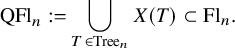
The union defining
$\mathrm {QFl}_{n}$
 is not disjoint as there is some overlap between distinct
$X(T)$
is not disjoint as there is some overlap between distinct
$X(T)$
 ,
$X(T')$
,
$X(T')$
 . In this section we characterize this overlap in terms of the torus fixed point sets
$I_{\widehat {F}}$
. In this section we characterize this overlap in terms of the torus fixed point sets
$I_{\widehat {F}}$
 described in Section 6.
Theorem 8.1. For
$\widehat {F},\widehat {G}\in \operatorname {BNestFor}_n$
 we have
$X(\widehat {G})\subset X(\widehat {F})$
we have
$X(\widehat {G})\subset X(\widehat {F})$
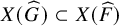 if and only if
$I_{\widehat {G}}\subset I_{\widehat {F}}$
if and only if
$I_{\widehat {G}}\subset I_{\widehat {F}}$
 .
.
The criterion therein provides a combinatorial model for the toric structure of
$\mathrm {QFl}_{n}$
 ; see Figure 6. First take the disjoint union of the moment polytopes for each
$X(T)$
; see Figure 6. First take the disjoint union of the moment polytopes for each
$X(T)$
 , which we showed in Section 5 are
$(n-1)$
, which we showed in Section 5 are
$(n-1)$
 -dimensional combinatorial cubes. Then create a polyhedral complex
$\mathrm {Complex}(\mathrm {QFl}_{n})$
-dimensional combinatorial cubes. Then create a polyhedral complex
$\mathrm {Complex}(\mathrm {QFl}_{n})$
 by identifying faces from distinct polytopes that are equal in the sense that they share the same set of vertices. After identification, the faces of
$\mathrm {Complex}(\mathrm {QFl}_{n})$
by identifying faces from distinct polytopes that are equal in the sense that they share the same set of vertices. After identification, the faces of
$\mathrm {Complex}(\mathrm {QFl}_{n})$
 are then in bijection with the distinct torus orbit closures in
$\mathrm {QFl}_n$
are then in bijection with the distinct torus orbit closures in
$\mathrm {QFl}_n$
 .
.
The combinatorial cubes corresponding to the toric orbit closures in each of the two components of
$\mathrm {QFl}_3$
 (left) and the global complex
$\mathrm {Complex}(\mathrm {QFl}_{3})$
(left) and the global complex
$\mathrm {Complex}(\mathrm {QFl}_{3})$
 encoding the inclusion order on all toric closures
$X(\widehat {F})$
encoding the inclusion order on all toric closures
$X(\widehat {F})$
 in
$\mathrm {QFl}_3$
in
$\mathrm {QFl}_3$
 (right).
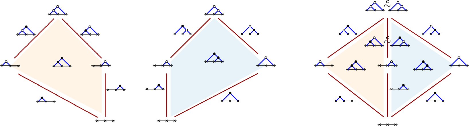
Figure 6 Long description
A three-panel diagram illustrating mathematical complexes.
Panel 1 (Left): A light orange pentagonal region outlined by dark red segments. Seven small tree diagrams are positioned around and inside it. At the top vertex is a tree with an open circle root. Moving clockwise, trees with varying black and white nodes are placed at the vertices and midpoints of the edges. One tree is located in the center of the orange region.
Panel 2 (Middle): A light blue pentagonal region, mirrored horizontally compared to the first. It is also outlined by dark red segments and surrounded by seven tree diagrams. The arrangement mirrors the first panel, with a central tree diagram inside the blue region.
Panel 3 (Right): A global complex formed by joining the orange and blue regions along a shared vertical central axis. The two regions are separated by a small gap containing two vertical red segments. Above the top vertex, two tree diagrams are joined by a tilde symbol with a small letter c above it. A similar tilde-c connection appears between two trees in the upper-middle section. The surrounding tree diagrams from the previous panels are preserved in their respective positions relative to the colored regions. At the very bottom, a single tree diagram consisting of three horizontal marks serves as the base for both components.
We prove Theorem 8.1 at the end of Section 8.2 after introducing an important equivalence relation on
$\operatorname {BNestFor}_n$
 in Section 8.1. Section 8.3 contains further enumerative and structural results about
$\mathrm {Complex}(\mathrm {QFl}_{n})$
in Section 8.1. Section 8.3 contains further enumerative and structural results about
$\mathrm {Complex}(\mathrm {QFl}_{n})$
 .
.
8.1 Colored Tamari equivalence and normal forms
Every torus orbit closure in
$\mathrm {QFl}_{n}$
 is by definition contained in
$X(T)$
is by definition contained in
$X(T)$
 for some
$T \in \mathrm {Tree}_{n}$
for some
$T \in \mathrm {Tree}_{n}$
 . In Section 5, we showed every torus orbit closure in
$X(T)$
. In Section 5, we showed every torus orbit closure in
$X(T)$
 is of the form
$X(\widehat {F})$
is of the form
$X(\widehat {F})$
 for a bicolored nested forest
$\widehat {F} \le _{re} T$
for a bicolored nested forest
$\widehat {F} \le _{re} T$
 . Thus the torus orbit closures in
$\mathrm {QFl}_{n}$
. Thus the torus orbit closures in
$\mathrm {QFl}_{n}$
 can be parametrized by
$\operatorname {BNestFor}_n$
can be parametrized by
$\operatorname {BNestFor}_n$
 . However, there is some redundancy in this parametrization as is apparent from Figure 6. This is explained by the following two additional relations that the building operations satisfy.
Lemma 8.2. For all
$1 \le i < n$
 we have the relations

Proof. Both relations can be verified with elementary matrix computations.
In the correspondence between words in
$\mathrm {RTSeq}_n$
 and compositions of building operations, these relations correspond to
$\mathsf {e}_{i} \mathsf {r}_{i+1}^+=\mathsf {r}_{i}^+ \mathsf {e}_{i}$
and compositions of building operations, these relations correspond to
$\mathsf {e}_{i} \mathsf {r}_{i+1}^+=\mathsf {r}_{i}^+ \mathsf {e}_{i}$
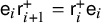 and
$\mathsf {r}_{i}^+ \mathsf {r}_{i+1}^+=\mathsf {r}_{i}^+ \mathsf {r}_{i}^+$
and
$\mathsf {r}_{i}^+ \mathsf {r}_{i+1}^+=\mathsf {r}_{i}^+ \mathsf {r}_{i}^+$
 . Considering the relations at the level of binary forests leads to the following definition.
Definition 8.3. We say that
$\widehat {F}, \widehat {G}\in \operatorname {BNestFor}_n$
 are
$\color {blue}{{colored\, Tamari\, equivalent}}$
are
$\color {blue}{{colored\, Tamari\, equivalent}}$
 , denoted by
$\widehat {F}\overset {c}{\sim } \widehat {G}$
, denoted by
$\widehat {F}\overset {c}{\sim } \widehat {G}$
 , if one can be transformed into the other by a sequence of
$\color {blue}{{colored\, Tamari\, rotations}}$
, if one can be transformed into the other by a sequence of
$\color {blue}{{colored\, Tamari\, rotations}}$
 shown below.

By the preceding discussion, we get the following result.
Proposition 8.4. If
$\widehat {F},\widehat {G}\in \operatorname {BNestFor}$
 satisfy
$\widehat {F}\overset {c}{\sim } \widehat {G}$
satisfy
$\widehat {F}\overset {c}{\sim } \widehat {G}$
 , then
$X(\widehat {F})=X(\widehat {G})$
, then
$X(\widehat {F})=X(\widehat {G})$
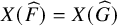 , and in particular
$I_{\widehat {F}}=I_{\widehat {G}}$
, and in particular
$I_{\widehat {F}}=I_{\widehat {G}}$
 .
.
Definition 8.5. We say that
$\widehat {F} \in \operatorname {BNestFor}_{n}$
 is in
$\color {blue}{{normal\, form}}$
is in
$\color {blue}{{normal\, form}}$
 if every right child in
$\operatorname {IN}(\widehat {F})$
if every right child in
$\operatorname {IN}(\widehat {F})$
 is a black node. Let
$\color {blue}{\mathrm{BNestFor}^{\mathrm {nf}}_n}$
is a black node. Let
$\color {blue}{\mathrm{BNestFor}^{\mathrm {nf}}_n}$
 be the set of bicolored nested forests that are in normal form.
Every element of
$\operatorname {BNestFor}_n$
 can be transformed to some element of
$\operatorname {BNestFor}^{\operatorname {nf}}_n$
can be transformed to some element of
$\operatorname {BNestFor}^{\operatorname {nf}}_n$
 by applying colored Tamari rotations repeatedly. We will prove that this normal form is unique in the next section. Figure 7 depicts a bicolored tree as well as its colored Tamari equivalent normal form.
Remark 8.6. Proposition 6.3 relates bicolored nested forests to factorizations of noncrossing partitions, where the colored Tamari equivalence allows certain relations
$(i\,k)(j\,k)=(j\,k)(i\,j)$
 .
.
A bicolored tree which is not in normal form (left), its Tamari-equivalent normal form (right), and the associated factorizations of
$\boldsymbol {c}$
 for each tree (below).
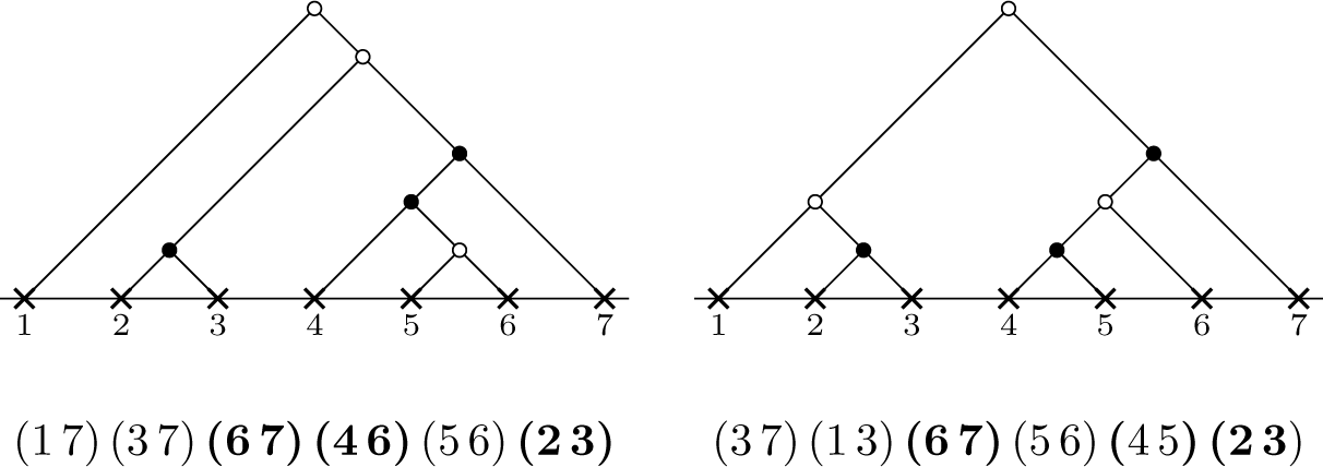
Figure 7 Long description
The image contains two panels.
Left panel: A bicolored tree with a root at the top represented by a white circle. The tree branches down to the right to another white circle, which then branches to a black circle. From this black circle, branches lead to another black circle and then a white circle. The leaves are marked with crosses on a horizontal line numbered 1 through 7. The structure is skewed heavily to the right. Below this tree is the factorization: (1 7) (3 7) bold (6 7) (4 6) (5 6) bold (2 3).
Right panel: The Tamari-equivalent normal form tree. It has a more balanced, symmetric structure. The root is a white circle at the top. It branches left to a white circle and right to a black circle. The left branch further divides into a black circle. The right branch further divides into a white circle and then a black circle. The leaves are similarly marked with crosses on a horizontal line numbered 1 through 7. Below this tree is the factorization: (3 7) (1 3) bold (6 7) (5 6) (4 5) bold (2 3).
In both trees, nodes are either hollow white circles or solid black circles, and the leaf nodes 1 through 7 serve as the base anchors.
8.2 The Bruhat maximal element of
$X(\widehat {F})$
and uniqueness of normal form

We will need to understand the Bruhat order on
$I_{\widehat {F}}$
 . Since
$X(\widehat {F})$
. Since
$X(\widehat {F})$
 is a torus orbit closure in
$\mathrm {Fl}_{n}$
is a torus orbit closure in
$\mathrm {Fl}_{n}$
 , we have that
$I_{\widehat {F}}$
, we have that
$I_{\widehat {F}}$
 is a flag matroid [Reference Gelfand, Goresky, MacPherson and Serganova22]. Hence we have the following fact.
Fact 8.7 [Reference Borovik, Gelfand and White16, § 1.9]
For any
$\widehat {F}\in \operatorname {BNestFor}_n$
 ,
$I_{\widehat {F}}$
,
$I_{\widehat {F}}$
 has a unique Bruhat-maximum element. This element is characterized by the property that all adjacent vertices are lower in the Bruhat order.
In order to describe this distinguished element, we define a new map. For
$\widehat {F}$
 in
$\operatorname {BNestFor}^{\operatorname {nf}}_n$
in
$\operatorname {BNestFor}^{\operatorname {nf}}_n$
 , let
$\text{ RC } (\widehat {F})$
, let
$\text{ RC } (\widehat {F})$
 denote the set of internal nodes that are right children. By definition of normal form, we note that all nodes in
$\text{ RC } (\widehat {F})$
denote the set of internal nodes that are right children. By definition of normal form, we note that all nodes in
$\text{ RC } (\widehat {F})$
 are black. We define a map

where
$\widehat {F} \setminus \text{ RC } (\widehat {F})$
 denotes the bicolored nested forest obtained by left edge deletion for each node
$v \in \text{ RC } (\widehat {F})$
denotes the bicolored nested forest obtained by left edge deletion for each node
$v \in \text{ RC } (\widehat {F})$
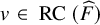 and contracting it in the sense of Proposition 5.4. This is a natural extension of the map on
$\operatorname {\mathsf {Forest}}_n$
and contracting it in the sense of Proposition 5.4. This is a natural extension of the map on
$\operatorname {\mathsf {Forest}}_n$
 which we defined in [Reference Bergeron, Gagnon, Nadeau, Spink and Tewari6, Section 7.2] using the same notation.
Example 8.8. We have

Lemma 8.9. For
$\widehat {F} = \widehat {G} \cdot \mathsf {x}_{i} \in \operatorname {BNestFor}^{\operatorname {nf}}_{n}$
 with
$\widehat {G}\in \operatorname {BNestFor}^{\operatorname {nf}}_{n-1}$
with
$\widehat {G}\in \operatorname {BNestFor}^{\operatorname {nf}}_{n-1}$
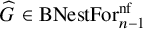 , we have

Proof. From the definitions we immediately verify

after which the formulas (6.1) complete the proof.
Proposition 8.10. If
$\widehat {F} \in \operatorname {BNestFor}^{\operatorname {nf}}_n$
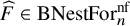 , then
$\operatorname {ForToNC}(\widehat {F})$
, then
$\operatorname {ForToNC}(\widehat {F})$
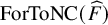 is the Bruhat-maximum element of
$I_{\widehat {F}}$
is the Bruhat-maximum element of
$I_{\widehat {F}}$
 .
.
Proof. We proceed by induction on n. For
$n = 1$
 ,
$\operatorname {ForToNC}(\widehat {F})$
,
$\operatorname {ForToNC}(\widehat {F})$
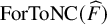 is the only element of
$I_{\widehat {F}}$
is the only element of
$I_{\widehat {F}}$
 . For
$n> 1$
. For
$n> 1$
 , we have
$\widehat {F} = \widehat {G} \cdot \mathsf {x}_{i}$
, we have
$\widehat {F} = \widehat {G} \cdot \mathsf {x}_{i}$
 for
$\mathsf {x}_{i} \in \{\mathsf {r}_{i}^{\pm }, \mathsf {e}_{i}\}$
for
$\mathsf {x}_{i} \in \{\mathsf {r}_{i}^{\pm }, \mathsf {e}_{i}\}$
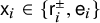 and
$\widehat {G}\in \operatorname {BNestFor}^{\operatorname {nf}}_{n-1}$
and
$\widehat {G}\in \operatorname {BNestFor}^{\operatorname {nf}}_{n-1}$
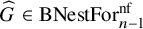 . Setting
$w = \operatorname {ForToNC}(\widehat {F})$
. Setting
$w = \operatorname {ForToNC}(\widehat {F})$
 and
$u = \operatorname {ForToNC}(\widehat {G})$
and
$u = \operatorname {ForToNC}(\widehat {G})$
 , Lemma 8.9 states that
$w = \Psi ^{\epsilon }_{i}(u)$
, Lemma 8.9 states that
$w = \Psi ^{\epsilon }_{i}(u)$
 for
$\epsilon \in \{+, -\}$
for
$\epsilon \in \{+, -\}$
 .
.
An example of the construction in Proposition 8.11 for
$n=12$
 (left) and all elements
$\widehat {(F,S)}\in \operatorname {BNestFor}^{\operatorname {nf}}_4$
(left) and all elements
$\widehat {(F,S)}\in \operatorname {BNestFor}^{\operatorname {nf}}_4$
 for
$F = \widehat {F}(\mathsf {r}_{1}^{-}\mathsf {e}_{1}\mathsf {e}_{1}\mathsf {e}_{3}) \in \operatorname {\mathsf {Forest}}_{4}$
for
$F = \widehat {F}(\mathsf {r}_{1}^{-}\mathsf {e}_{1}\mathsf {e}_{1}\mathsf {e}_{3}) \in \operatorname {\mathsf {Forest}}_{4}$
 (right).
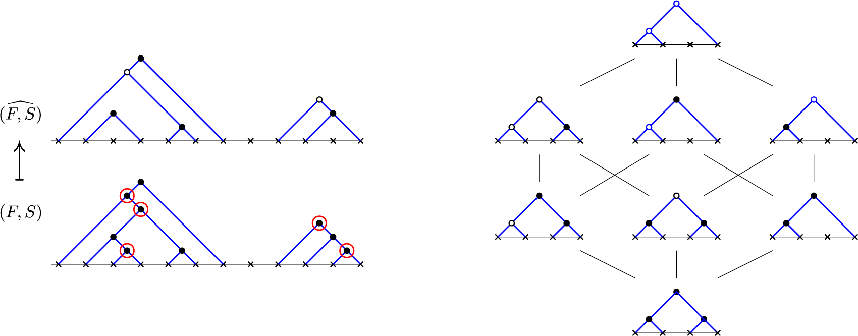
Figure 8 Long description
The left panel displays a vertical mapping. At the bottom is a forest structure labeled (F, S) consisting of two blue-lined trees over a horizontal axis marked with x symbols. Five nodes in this forest are circled in red. An upward arrow with a bar at the base points to the top structure labeled (F hat, S). In this top version, the red circles are removed, and some solid black nodes have been replaced with hollow white nodes.
The right panel is a Hasse diagram showing a lattice of eight individual forest elements.
* At the top level is a single forest with two hollow white nodes.
* The second level down contains three forests connected to the top by lines, showing different combinations of one solid black node and one hollow white node.
* The third level down contains three forests, showing further variations with more solid black nodes.
* At the bottom level is a single forest where the primary nodes are solid black.
Each forest in the lattice is composed of blue lines connecting nodes over a base of four x marks on a horizontal line.
For
$\mathsf {x}_{i} = \mathsf {r}_{i}^{\epsilon }$
 , we note that both
$\Psi _{i}^{-}$
, we note that both
$\Psi _{i}^{-}$
 and
$\Psi _{i}^{+}$
and
$\Psi _{i}^{+}$
 preserve the Bruhat order. This follows, for instance, from the tableau criterion [Reference Björner and Brenti14, Theorem 2.6.3]. Thus, using our inductive hypothesis on u, we have that
$w = \Psi ^{\epsilon }_{i}(u)$
preserve the Bruhat order. This follows, for instance, from the tableau criterion [Reference Björner and Brenti14, Theorem 2.6.3]. Thus, using our inductive hypothesis on u, we have that
$w = \Psi ^{\epsilon }_{i}(u)$
 is the Bruhat maximum of
$I_{\widehat {F}} = \Psi ^{\epsilon }_{i}(I_{\widehat {G}})$
is the Bruhat maximum of
$I_{\widehat {F}} = \Psi ^{\epsilon }_{i}(I_{\widehat {G}})$
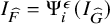 .
.
Now suppose that
$\mathsf {x}_{i} = \mathsf {e}_{i}$
 . By Fact 8.7, it suffices to show that w is greater than all adjacent fixed points in
$I_{\widehat {F}}$
. By Fact 8.7, it suffices to show that w is greater than all adjacent fixed points in
$I_{\widehat {F}}$
 . As
$I_{\widehat {F}}$
. As
$I_{\widehat {F}}$
 is a combinatorial cube and
$\Psi ^{\epsilon }_{i}$
is a combinatorial cube and
$\Psi ^{\epsilon }_{i}$
 is a face inclusion, all but one of these adjacent elements are contained in
$\Psi ^{\epsilon }_{i}(I_{\widehat {G}})$
is a face inclusion, all but one of these adjacent elements are contained in
$\Psi ^{\epsilon }_{i}(I_{\widehat {G}})$
 and therefore covered by the previous argument. The remaining adjacent fixed point is
$ws_{i}$
and therefore covered by the previous argument. The remaining adjacent fixed point is
$ws_{i}$
 , so what remains is to show that
$w(i)> w(i+1)$
, so what remains is to show that
$w(i)> w(i+1)$
 . Let v be the (black) node associated to
$\mathsf {x}_{i}$
. Let v be the (black) node associated to
$\mathsf {x}_{i}$
 . If v is a right child in
$\widehat {F}$
. If v is a right child in
$\widehat {F}$
 , then
$w(i) = i$
, then
$w(i) = i$
 and
$w(i+1) < i+1$
and
$w(i+1) < i+1$
 . If v is not a right child, then i is the smallest element of its cycle, which must also contain
$i+1$
. If v is not a right child, then i is the smallest element of its cycle, which must also contain
$i+1$
 , so again
$w(i)> w(i+1)$
, so again
$w(i)> w(i+1)$
 .
.
We need an alternative construction related to the map
$\operatorname {ForToNC}$
 . Let
$(F,S)$
. Let
$(F,S)$
 be a pair consisting of an indexed forest
$F\in \operatorname {\mathsf {Forest}}_n$
be a pair consisting of an indexed forest
$F\in \operatorname {\mathsf {Forest}}_n$
 and a subset
$S \subseteq \operatorname {IN}(F)$
and a subset
$S \subseteq \operatorname {IN}(F)$
 . We define

by performing left-edge deletion on all vertices in
$S\cap \text{ RC } (F)$
 , and coloring the remaining vertices of S white. An example is shown in Figure 8 (left).
Proposition 8.11. The map
$(F,S)\mapsto \widehat {(F,S)}$
 is a bijection from
$\{(F, S) \;|\; F \in \operatorname {\mathsf {Forest}}_{n}, S \subseteq \operatorname {IN}(F)\}$
is a bijection from
$\{(F, S) \;|\; F \in \operatorname {\mathsf {Forest}}_{n}, S \subseteq \operatorname {IN}(F)\}$
 onto
$\operatorname {BNestFor}^{\operatorname {nf}}_n$
onto
$\operatorname {BNestFor}^{\operatorname {nf}}_n$
 . Furthermore,
$\operatorname {ForToNC}\widehat {(F,S)}=\operatorname {ForToNC}(F)$
. Furthermore,
$\operatorname {ForToNC}\widehat {(F,S)}=\operatorname {ForToNC}(F)$
 for all
$(F, S)$
for all
$(F, S)$
 .
.
Proof. The fact that
$\operatorname {ForToNC}\widehat {(F,S)}=\operatorname {ForToNC}(F)$
 follows from the definition of
$\operatorname {ForToNC}$
follows from the definition of
$\operatorname {ForToNC}$
 . For fixed F, the forests
$\widehat {(F,S)}$
. For fixed F, the forests
$\widehat {(F,S)}$
 are distinct as they correspond to distinct elements of
$\mathrm {Face}(F)$
are distinct as they correspond to distinct elements of
$\mathrm {Face}(F)$
 : given a fixed sequence
$(\mathsf {r}_{1}^-)^{n-k}e_{i_1}\cdots e_{i_k}$
: given a fixed sequence
$(\mathsf {r}_{1}^-)^{n-k}e_{i_1}\cdots e_{i_k}$
 for F, the choice of S determines the subset of
$e_{i_1},\ldots ,e_{i_k}$
for F, the choice of S determines the subset of
$e_{i_1},\ldots ,e_{i_k}$
 to transform to
$\mathsf {r}_{i}^{\pm }$
to transform to
$\mathsf {r}_{i}^{\pm }$
 . This shows that the map
$(F,S)\mapsto \widehat {(F,S)}$
. This shows that the map
$(F,S)\mapsto \widehat {(F,S)}$
 is an injection, so it remains to construct an inverse map. Given
$\widehat {G}$
is an injection, so it remains to construct an inverse map. Given
$\widehat {G}$
 in
$\operatorname {BNestFor}^{\operatorname {nf}}_n$
in
$\operatorname {BNestFor}^{\operatorname {nf}}_n$
 , we create
$G\in \operatorname {\mathsf {Forest}}_n$
, we create
$G\in \operatorname {\mathsf {Forest}}_n$
 by coloring all of its vertices black and then connecting the remaining nested trees using the procedure described below.
For each
$v\in \operatorname {IN}(\widehat {G})$
 , let
$T_1,\ldots ,T_k$
, let
$T_1,\ldots ,T_k$
 be the outermost trees which are nested in the subtree below v, listed from left to right. Denoting their roots
$w_1,\ldots ,w_k$
be the outermost trees which are nested in the subtree below v, listed from left to right. Denoting their roots
$w_1,\ldots ,w_k$
 , we create new black nodes
$v_1',\ldots ,v_k'$
, we create new black nodes
$v_1',\ldots ,v_k'$
 in the interior of the edge from v to
$v_R$
in the interior of the edge from v to
$v_R$
 in this order, and then for each i we connect
$w_i$
in this order, and then for each i we connect
$w_i$
 to
$v_i'$
to
$v_i'$
 .
.
The resulting forest G does not depend on the order in which we apply the connection procedure. Setting
$S \subseteq \operatorname {IN}(G)$
 to be the set consisting of the newly created nodes together with the black nodes that came from white nodes of
$\widehat {G}$
to be the set consisting of the newly created nodes together with the black nodes that came from white nodes of
$\widehat {G}$
 ,
$\widehat {G}\mapsto (G,S)$
,
$\widehat {G}\mapsto (G,S)$
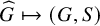 is the inverse map.
Proposition 8.12. Let
$\widehat {F},\widehat {G}\in \operatorname {BNestFor}^{\operatorname {nf}}_{n}$
 . If
$I_{\widehat {F}}=I_{\widehat {G}}$
. If
$I_{\widehat {F}}=I_{\widehat {G}}$
 , then
$\widehat {F}=\widehat {G}$
, then
$\widehat {F}=\widehat {G}$
 .
.
Proof. We show that we can reconstruct
$\widehat {F}$
 from
$I=I_{\widehat {F}}$
from
$I=I_{\widehat {F}}$
 . First, we recover
$w=\operatorname {ForToNC}(\widehat {F})$
. First, we recover
$w=\operatorname {ForToNC}(\widehat {F})$
 as the maximal element in I with respect to the Bruhat order by Proposition 8.10. By Proposition 8.11, this means
$\widehat {F}=\widehat {(F,S)}$
as the maximal element in I with respect to the Bruhat order by Proposition 8.10. By Proposition 8.11, this means
$\widehat {F}=\widehat {(F,S)}$
 for the unique
$F \in \operatorname {\mathsf {Forest}}_{n}$
for the unique
$F \in \operatorname {\mathsf {Forest}}_{n}$
 with
$\operatorname {ForToNC}(F) = w$
with
$\operatorname {ForToNC}(F) = w$
 and some unique
$S\subset \operatorname {IN}(F)$
and some unique
$S\subset \operatorname {IN}(F)$
 so it remains to show that the
$I_{\widehat {(F,S)}}$
so it remains to show that the
$I_{\widehat {(F,S)}}$
 are distinct for fixed F. Indeed, by Proposition 8.11 again, as we vary S we obtain distinct
$\widehat {(F,S)}\in \mathrm {Face}(F)$
are distinct for fixed F. Indeed, by Proposition 8.11 again, as we vary S we obtain distinct
$\widehat {(F,S)}\in \mathrm {Face}(F)$
 , so we conclude the vertex sets
$I_{\widehat {(F,S)}}$
, so we conclude the vertex sets
$I_{\widehat {(F,S)}}$
 are distinct as a face is determined by its vertex set.
Remark 8.13. One can show that
$I_{\widehat {(F,S)}}$
 is the smallest sublattice of
$I_F$
is the smallest sublattice of
$I_F$
 which contains
$\operatorname {ForToNC}(F)$
which contains
$\operatorname {ForToNC}(F)$
 and
$\operatorname {NCPerm}(\widehat {(F,S)}\setminus A)$
and
$\operatorname {NCPerm}(\widehat {(F,S)}\setminus A)$
 for
$A\subset \operatorname {IN}(\widehat {(F,S)})$
for
$A\subset \operatorname {IN}(\widehat {(F,S)})$
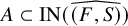 , the subset of black nodes that are not right children.
Proposition 8.14. Every colored Tamari equivalence class in
$\operatorname {BNestFor}_n$
 has a unique normal form representative in
$\operatorname {BNestFor}^{\operatorname {nf}}_n$
has a unique normal form representative in
$\operatorname {BNestFor}^{\operatorname {nf}}_n$
 . Moreover, for
$\widehat {F},\widehat {G}\in \operatorname {BNestFor}_n$
. Moreover, for
$\widehat {F},\widehat {G}\in \operatorname {BNestFor}_n$
 , the following are equivalent:
-
(1) $X(\widehat {F})=X(\widehat {G})$
, -
(2) $\widehat {F}{\overset {c}{\sim }} \widehat {G}$
, and -
(3) $I_{\widehat {F}}=I_{\widehat {G}}$
.
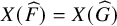


Proof. If
$\widehat {F}\overset {c}{\sim } \widehat {G}$
 are both in normal form, then by Proposition 8.4 we have
$X(\widehat {F})=X(\widehat {G})$
are both in normal form, then by Proposition 8.4 we have
$X(\widehat {F})=X(\widehat {G})$
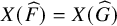 , and in particular
$I_{\widehat {F}}=I_{\widehat {G}}$
, and in particular
$I_{\widehat {F}}=I_{\widehat {G}}$
 and so by Proposition 8.12 we conclude that
$\widehat {F}=\widehat {G}$
and so by Proposition 8.12 we conclude that
$\widehat {F}=\widehat {G}$
 .
.
We know already that (2) implies (1) by Proposition 8.4, and obviously (1) implies (3). It remains only to show that (3) implies (2). By Proposition 8.4, colored Tamari rotations preserve
$I_{\widehat {F}}$
 . Let
$\widehat {F}'$
. Let
$\widehat {F}'$
 and
$\widehat {G}'$
and
$\widehat {G}'$
 be the normal form colored Tamari equivalents to
$\widehat {F}$
be the normal form colored Tamari equivalents to
$\widehat {F}$
 and
$\widehat {G}$
and
$\widehat {G}$
 . Then
$I_{\widehat {F}'}=I_{\widehat {G}'}$
. Then
$I_{\widehat {F}'}=I_{\widehat {G}'}$
 and so by Proposition 8.12 we deduce that
$\widehat {F}'=\widehat {G}'$
and so by Proposition 8.12 we deduce that
$\widehat {F}'=\widehat {G}'$
 , and so conclude that
$\widehat {F}{\overset {c}{\sim }} \widehat {G}$
, and so conclude that
$\widehat {F}{\overset {c}{\sim }} \widehat {G}$
 .
.
We are now ready to prove Theorem 8.1.
Proof of Theorem 8.1
Clearly,
$X(\widehat {G}) \subset X(\widehat {F})$
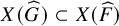 implies
$I_{\widehat {G}}\subset I_{\widehat {F}}$
implies
$I_{\widehat {G}}\subset I_{\widehat {F}}$
 . Suppose now
$I_{\widehat {G}}\subset I_{\widehat {F}}$
. Suppose now
$I_{\widehat {G}}\subset I_{\widehat {F}}$
 . By Corollary 6.4, both
$I_{\widehat {G}}$
. By Corollary 6.4, both
$I_{\widehat {G}}$
 and
$I_{\widehat {F}}$
and
$I_{\widehat {F}}$
 are boolean lattices inside the Kreweras lattice. Recall the absolute length of a noncrossing partition
$w\in \operatorname {NC}_n$
are boolean lattices inside the Kreweras lattice. Recall the absolute length of a noncrossing partition
$w\in \operatorname {NC}_n$
 is n minus the number of cycles of w, which is the minimal number of transpositions needed to multiply to w. Let
$u, v \in I_{\widehat {G}}$
is n minus the number of cycles of w, which is the minimal number of transpositions needed to multiply to w. Let
$u, v \in I_{\widehat {G}}$
 be the top and bottom elements in the Kreweras order, of absolute lengths a and b respectively, so that
$|I_{\widehat {G}}|=2^{a-b}$
be the top and bottom elements in the Kreweras order, of absolute lengths a and b respectively, so that
$|I_{\widehat {G}}|=2^{a-b}$
 . On the other hand the set of permutations in
$I_{\widehat {F}}$
. On the other hand the set of permutations in
$I_{\widehat {F}}$
 between u and v in the Kreweras order is a subinterval of
$I_{\widehat {F}}$
between u and v in the Kreweras order is a subinterval of
$I_{\widehat {F}}$
 with
$2^{a-b}$
with
$2^{a-b}$
 elements. It follows that
$I_{\widehat {G}}$
elements. It follows that
$I_{\widehat {G}}$
 is this subinterval of
$I_{\widehat {F}}$
is this subinterval of
$I_{\widehat {F}}$
 , so there exists
$\widehat {G}'\in \mathrm {Face}(\widehat {F})$
, so there exists
$\widehat {G}'\in \mathrm {Face}(\widehat {F})$
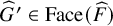 with
$I_{\widehat {G}}=I_{\widehat {G}'}$
with
$I_{\widehat {G}}=I_{\widehat {G}'}$
 . By Proposition 8.14 this implies
$X(\widehat {G}')=X(\widehat {G}) \subset X(\widehat {F})$
. By Proposition 8.14 this implies
$X(\widehat {G}')=X(\widehat {G}) \subset X(\widehat {F})$
 .
.
8.3 Combinatorics of torus orbit closures
In this section, we describe several enumerative aspects of the complex
$\mathrm {Complex}(\mathrm {QFl}_{n})$
 . We moreover show in Proposition 8.15 that the number of such orbits for
$n=1,2,3,\ldots $
. We moreover show in Proposition 8.15 that the number of such orbits for
$n=1,2,3,\ldots $
 is given by generalized Catalan numbers [Reference Sloane42, A064062], while counting them according to dimension gives a refinement known as
$\color {blue}{{Borel's\, triangle}}$
is given by generalized Catalan numbers [Reference Sloane42, A064062], while counting them according to dimension gives a refinement known as
$\color {blue}{{Borel's\, triangle}}$
 [Reference Sloane42, A234950].
We now describe the cell structure of
$\mathrm {Complex}(\mathrm {QFl}_{n})$
 . In general the intersection of two torus orbit closures under inclusion is a union of one or more torus orbit closures. As shown on the right in Figure 6, the intersection of the top-dimensional orbit closures in
$\mathrm {Complex}(\mathrm {QFl}_{3})$
. In general the intersection of two torus orbit closures under inclusion is a union of one or more torus orbit closures. As shown on the right in Figure 6, the intersection of the top-dimensional orbit closures in
$\mathrm {Complex}(\mathrm {QFl}_{3})$
 is the (nondisjoint) union of two intervals. Theorem 8.1 shows that faces of
$\mathrm {Complex}(\mathrm {QFl}_{n})$
is the (nondisjoint) union of two intervals. Theorem 8.1 shows that faces of
$\mathrm {Complex}(\mathrm {QFl}_{n})$
 are in bijection with the fixed point sets
$I_{\widehat {F}} \subseteq \operatorname {NC}_{n}$
are in bijection with the fixed point sets
$I_{\widehat {F}} \subseteq \operatorname {NC}_{n}$
 for
$\widehat {F}\in \operatorname {BNestFor}_n$
for
$\widehat {F}\in \operatorname {BNestFor}_n$
 , with inclusion of faces corresponding to inclusion of sets. The faces are also in bijection with normal form forests in
$\operatorname {BNestFor}^{\operatorname {nf}}_n$
, with inclusion of faces corresponding to inclusion of sets. The faces are also in bijection with normal form forests in
$\operatorname {BNestFor}^{\operatorname {nf}}_n$
 , but inclusion is harder to compute with these objects; in particular it is strictly stronger than the restriction of the order
$\le _{re}$
, but inclusion is harder to compute with these objects; in particular it is strictly stronger than the restriction of the order
$\le _{re}$
 .
.
Proposition 8.15. Let
$G(z,u)=\sum _{n,k\geq 0}f_{n,k}z^nu^k$
 , where
$f_{n,k}$
, where
$f_{n,k}$
 is the number of torus orbits in
$\mathrm {QFl}_n$
is the number of torus orbits in
$\mathrm {QFl}_n$
 of dimension k. Then

Proof. We have that
$f_{n,k}$
 is the number of
$\widehat {F}\in \operatorname {BNestFor}^{\operatorname {nf}}_n$
is the number of
$\widehat {F}\in \operatorname {BNestFor}^{\operatorname {nf}}_n$
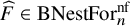 with k black nodes. First, let
$G_{\boldsymbol {c}}(z,u)$
with k black nodes. First, let
$G_{\boldsymbol {c}}(z,u)$
 be the generating function for trees
$T \in \operatorname {BNestFor}^{\operatorname {nf}}_n$
be the generating function for trees
$T \in \operatorname {BNestFor}^{\operatorname {nf}}_n$
 , so that
$\operatorname {NCPerm}(T)=\boldsymbol {c}$
, so that
$\operatorname {NCPerm}(T)=\boldsymbol {c}$
 . Decomposition at the root gives a quadratic functional equation for
$G_{\boldsymbol {c}}(z,u)$
. Decomposition at the root gives a quadratic functional equation for
$G_{\boldsymbol {c}}(z,u)$
 that has the solution

For the general case, note that each
$\widehat {F} \in \operatorname {BNestFor}^{\operatorname {nf}}_n$
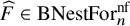 is given by the choice of an element
$w\in \operatorname {NC}_{n}$
is given by the choice of an element
$w\in \operatorname {NC}_{n}$
 and for each cycle
$C = (c_{1}\,\cdots \,c_{k})$
and for each cycle
$C = (c_{1}\,\cdots \,c_{k})$
 of w, a tree in
$\operatorname {BNestFor}^{\operatorname {nf}}_k$
of w, a tree in
$\operatorname {BNestFor}^{\operatorname {nf}}_k$
 . As in [Reference Chapoton and Nadeau18, §2.2], we can therefore apply the R-transform from free probability to obtain the equation
$G(z,u)=G_{\boldsymbol {c}}(zG(z,u),u)$
. As in [Reference Chapoton and Nadeau18, §2.2], we can therefore apply the R-transform from free probability to obtain the equation
$G(z,u)=G_{\boldsymbol {c}}(zG(z,u),u)$
 . This can be solved using the quadratic equation for
$G_{\boldsymbol {c}}(z,u)$
. This can be solved using the quadratic equation for
$G_{\boldsymbol {c}}(z,u)$
 , from which we obtain the desired result.
The expression (8.1) is the generating function for Borel’s triangle [Reference Sloane42, A234950] whose entries have the explicit closed form

From the expression (8.2), it follows that the enumeration for trees is given by the classical
$\color {blue}{{large\, Schr\unicode{x00F6}der\, numbers}}$
 [Reference Sloane42, A006318] and the refined version according to
$|\widehat {F}|$
[Reference Sloane42, A006318] and the refined version according to
$|\widehat {F}|$
 is [Reference Sloane42, A088617].
Remark 8.16. For comparison, every face of the complex attached to the complex
$\operatorname {HHMP}_n$
 discussed in the introduction is a cube, and intersections of faces are faces. These are indexed bijectively by the words in
$\mathrm {RESeq}_n$
discussed in the introduction is a cube, and intersections of faces are faces. These are indexed bijectively by the words in
$\mathrm {RESeq}_n$
 without any
$\mathsf {r}_{i}^{+}$
without any
$\mathsf {r}_{i}^{+}$
 , and a face
$F_1$
, and a face
$F_1$
 contains a face
$F_2$
contains a face
$F_2$
 if the word for
$F_1$
if the word for
$F_1$
 can be transformed to that for
$F_2$
can be transformed to that for
$F_2$
 by changing some letters
$\mathsf {e}_{i}$
by changing some letters
$\mathsf {e}_{i}$
 to either
$\mathsf {r}_{i}^{-}$
to either
$\mathsf {r}_{i}^{-}$
 or
$\mathsf {r}_{i+1}^{-}$
or
$\mathsf {r}_{i+1}^{-}$
 . The total number of faces is
$1\cdot 3\cdot 5 \cdots (2n-1)$
. The total number of faces is
$1\cdot 3\cdot 5 \cdots (2n-1)$
 [Reference Sloane42, A001147], refined according to dimension by the generating polynomial
$(1)(2+t)(3+2t)\cdots (n+(n-1)t)$
[Reference Sloane42, A001147], refined according to dimension by the generating polynomial
$(1)(2+t)(3+2t)\cdots (n+(n-1)t)$
 .
.
9 The affine paving of
$\mathrm {QFl}_n$

We now describe a family of affine charts for
$\mathrm {QFl}_{n}$
 around each of its torus fixed points. We begin in Section 9.1 by defining the charts in terms of the Bott manifold structure of the
$X(\widehat {F})$
around each of its torus fixed points. We begin in Section 9.1 by defining the charts in terms of the Bott manifold structure of the
$X(\widehat {F})$
 and showing that they partition
$\mathrm {QFl}_{n}$
and showing that they partition
$\mathrm {QFl}_{n}$
 . Then in Section 9.2 we explicitly construct each chart and show that our partition can be equivalently obtained by intersecting
$\mathrm {QFl}_{n}$
. Then in Section 9.2 we explicitly construct each chart and show that our partition can be equivalently obtained by intersecting
$\mathrm {QFl}_{n}$
 with the Bruhat decomposition of
$\mathrm {Fl}_{n}$
with the Bruhat decomposition of
$\mathrm {Fl}_{n}$
 .
.
9.1 The paving
For each
$F\in \operatorname {\mathsf {Forest}}_n$
 , the Bott manifold structure of
$X(F)$
, the Bott manifold structure of
$X(F)$
 from Section 5 gives an affine chart
$C(F)$
from Section 5 gives an affine chart
$C(F)$
 around the T-fixed point
$\operatorname {ForToNC}(F)\in X(F)$
around the T-fixed point
$\operatorname {ForToNC}(F)\in X(F)$
 . Explicitly,
$C(F)$
. Explicitly,
$C(F)$
 is isomorphic to an affine space
$\mathbb {A}^{|F|}$
is isomorphic to an affine space
$\mathbb {A}^{|F|}$
 of dimension
$|F|$
of dimension
$|F|$
 and decomposes into sub-torus-orbits of
$X(F)$
and decomposes into sub-torus-orbits of
$X(F)$
 as
as
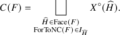
Theorem 9.1. The affine charts form a partition of
$\mathrm {QFl}_n$
 :
:
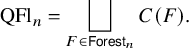
Moreover, for any total ordering
$F_1,F_2,\ldots ,F_{|\operatorname {NC}_{n}|}$
 of
$\operatorname {\mathsf {Forest}}_n$
of
$\operatorname {\mathsf {Forest}}_n$
 that extends the pullback of the Bruhat order via
$\operatorname {ForToNC}$
that extends the pullback of the Bruhat order via
$\operatorname {ForToNC}$
 , we have
$\bigsqcup _{i=1}^{k} C(F_{i})=\bigcup _{i=1}^k X(F_i)$
, we have
$\bigsqcup _{i=1}^{k} C(F_{i})=\bigcup _{i=1}^k X(F_i)$
 .
.
We prove the theorem after the following remark and lemma.
Remark 9.2. The decomposition in Theorem 9.1 can be interpreted as a partition of
$\mathrm {Complex}(\mathrm {QFl}_{n})$
 by associating each
$C(F)$
by associating each
$C(F)$
 with the half-open subspace of the moment polytope for
$X(F)$
with the half-open subspace of the moment polytope for
$X(F)$
 around the vertex
$\operatorname {ForToNC}(F)$
around the vertex
$\operatorname {ForToNC}(F)$
 ; see Figure 9.
The decomposition of
$\mathrm {Complex}(\mathrm {QFl}_{3})$
 induced by our affine paving of
$\mathrm {QFl}_{3}$
induced by our affine paving of
$\mathrm {QFl}_{3}$
 as described in Remark 9.2; compare to Figure 6.
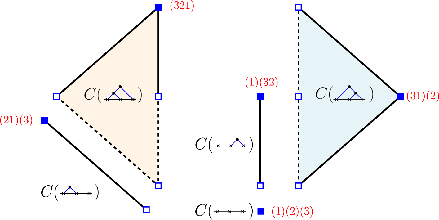
Figure 9 Long description
The diagram consists of four distinct geometric components arranged horizontally.
1. Far-left panel: A large orange-shaded triangle and a separate diagonal line segment below it. The triangle has a solid top-right vertex labeled with a blue square and red text (3 2 1). Its interior is labeled C followed by a tree graph with a root node branching into two nodes. The line segment below it has a blue square vertex at the top-left labeled (2 1)(3) and is labeled C followed by a tree graph where the root is on the left.
2. Center-left panel: A vertical line segment with a solid blue square at the top labeled (1)(3 2) and an open square at the bottom. It is labeled C followed by a tree graph where the root is on the right.
3. Center-right panel: A large light-blue shaded triangle. Its rightmost vertex is a solid blue square labeled (3 1)(2). The interior is labeled C followed by a tree graph with a root node branching into two nodes, mirrored from the first triangle. The left edge of this triangle is a dashed line with open square vertices.
4. Far-right panel: A single solid blue square point at the bottom, labeled (1)(2)(3). It is labeled C followed by a horizontal line with three x marks and no branching tree structure.
Lemma 9.3. Let
$F\in \operatorname {\mathsf {Forest}}_n$
 and
$\widehat {H}\in \operatorname {BNestFor}^{\operatorname {nf}}_{n}$
and
$\widehat {H}\in \operatorname {BNestFor}^{\operatorname {nf}}_{n}$
 . Then
$\operatorname {ForToNC}(\widehat {H})=\operatorname {ForToNC}(F)$
. Then
$\operatorname {ForToNC}(\widehat {H})=\operatorname {ForToNC}(F)$
 if and only if
$\widehat {H} \in \mathrm {Face}(F)$
if and only if
$\widehat {H} \in \mathrm {Face}(F)$
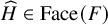 and
$\operatorname {ForToNC}(F) \in I_{\widehat {H}}$
and
$\operatorname {ForToNC}(F) \in I_{\widehat {H}}$
 .
.
Proof. If
$\operatorname {ForToNC}(\widehat {H})=\operatorname {ForToNC}(F)$
 , then
$\widehat {H}$
, then
$\widehat {H}$
 corresponds to a pair of the form
$(F,S)$
corresponds to a pair of the form
$(F,S)$
 by the construction of Proposition 8.11. It follows from the definition of
$\le _{re}$
by the construction of Proposition 8.11. It follows from the definition of
$\le _{re}$
 that
$\widehat {H} \in \mathrm {Face}(F)$
that
$\widehat {H} \in \mathrm {Face}(F)$
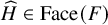 and likewise
$\operatorname {ForToNC}(F)\in I_{\widehat {H}}$
and likewise
$\operatorname {ForToNC}(F)\in I_{\widehat {H}}$
 . Conversely, if
$\widehat {H} \in \operatorname {BNestFor}^{\operatorname {nf}}_{n}$
. Conversely, if
$\widehat {H} \in \operatorname {BNestFor}^{\operatorname {nf}}_{n}$
 satisfies these two conditions, we know that
$I_{\widehat {H}}\subset I_{F}$
satisfies these two conditions, we know that
$I_{\widehat {H}}\subset I_{F}$
 by Theorem 8.1. Since
$\operatorname {ForToNC}(F)$
by Theorem 8.1. Since
$\operatorname {ForToNC}(F)$
 is the Bruhat-maximum element of
$I_F$
is the Bruhat-maximum element of
$I_F$
 by Proposition 8.10, it must be the Bruhat-maximum element of
$I_{\widehat {H}}$
by Proposition 8.10, it must be the Bruhat-maximum element of
$I_{\widehat {H}}$
 as well, which implies
$\operatorname {ForToNC}(\widehat {H})=\operatorname {ForToNC}(F)$
as well, which implies
$\operatorname {ForToNC}(\widehat {H})=\operatorname {ForToNC}(F)$
 by Proposition 8.10 again.
Proof of Theorem 9.1
By Proposition 8.14, we have
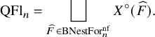
By Lemma 9.3 and Equation (9.1), we have
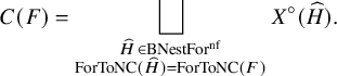
As
$\operatorname {ForToNC}$
 is surjective when restricted to
$\operatorname {\mathsf {Forest}}_{n}$
is surjective when restricted to
$\operatorname {\mathsf {Forest}}_{n}$
 , it follows immediately that Equation (9.4) coarsens the partition in Equation (9.3) into the one in Equation (9.2).
We now show that
$\bigcup _{i=1}^k C(F_i)=\bigcup _{j=1}^k X(F_j)$
 for any k. Since
$C(F)\subset X(F)$
for any k. Since
$C(F)\subset X(F)$
 for any
$F\in \operatorname {\mathsf {Forest}}$
for any
$F\in \operatorname {\mathsf {Forest}}$
 , we only have to show that any
$\mathcal {F}\in X(F_j)$
, we only have to show that any
$\mathcal {F}\in X(F_j)$
 for some
$j\leq k$
for some
$j\leq k$
 is included in
$C(F_i)$
is included in
$C(F_i)$
 for some
$i\leq k$
for some
$i\leq k$
 . We have
${\mathcal {F}\in X^{\circ }(\widehat {G})}$
. We have
${\mathcal {F}\in X^{\circ }(\widehat {G})}$
 for some
$\widehat {G}\in \operatorname {BNestFor}^{\operatorname {nf}}_n$
for some
$\widehat {G}\in \operatorname {BNestFor}^{\operatorname {nf}}_n$
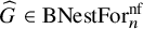 such that
$X^{\circ }(\widehat {G})\subset X(F_j)$
such that
$X^{\circ }(\widehat {G})\subset X(F_j)$
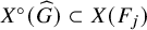 . By Theorem 8.1, this implies that
${I_{\widehat {G}}\subset I_{F_j}}$
. By Theorem 8.1, this implies that
${I_{\widehat {G}}\subset I_{F_j}}$
 . In particular, using the characterization of Proposition 8.10, we have
$\operatorname {ForToNC}(\widehat {G})\le \operatorname {ForToNC}(F_j)$
. In particular, using the characterization of Proposition 8.10, we have
$\operatorname {ForToNC}(\widehat {G})\le \operatorname {ForToNC}(F_j)$
 in Bruhat order. By our choice of total order we then have that
$\operatorname {ForToNC}(\widehat {G})=\operatorname {ForToNC}(F_i)$
in Bruhat order. By our choice of total order we then have that
$\operatorname {ForToNC}(\widehat {G})=\operatorname {ForToNC}(F_i)$
 for some
$i\leq j$
for some
$i\leq j$
 . Because of (9.4) we then have
$X^{\circ }(\widehat {G})\subset C(F_i)$
. Because of (9.4) we then have
$X^{\circ }(\widehat {G})\subset C(F_i)$
 , and thus
$\mathcal {F}\in C(F_i)$
, and thus
$\mathcal {F}\in C(F_i)$
 , which concludes the proof.
Remark 9.4 (Points over
$\mathbb {F}_q$
)

The definition of
$\mathrm {QFl}_n$
 and all arguments used so far make sense over any field, not just
$\mathbb {C}$
and all arguments used so far make sense over any field, not just
$\mathbb {C}$
 , and so using (9.2) and (9.3) we may count the number of points of
$\mathrm {QFl}_n$
, and so using (9.2) and (9.3) we may count the number of points of
$\mathrm {QFl}_n$
 over a finite field
$\mathbb {F}_q$
over a finite field
$\mathbb {F}_q$
 . In this case
$C(F)\simeq \mathbb {F}_q^{\operatorname {IN}(F)}$
. In this case
$C(F)\simeq \mathbb {F}_q^{\operatorname {IN}(F)}$
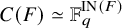 has cardinality
$q^{|F|}$
has cardinality
$q^{|F|}$
 . Summing over all
$F\in \operatorname {\mathsf {Forest}}_n$
. Summing over all
$F\in \operatorname {\mathsf {Forest}}_n$
 we get

where
$c_{n,k}=\frac {n-k}{n+k}\binom {n+k}{k}$
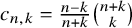 [Reference Nadeau and Tewari41]. Using (9.3) we get the alternative expression

where the numbers
$f_{n,k}$
 were introduced in Section 8.3. These two expressions are polynomial in q, and thus one can extract
$f_{n,k}=\sum _{m=k}^n\binom {m}{k}c_{n,m}$
were introduced in Section 8.3. These two expressions are polynomial in q, and thus one can extract
$f_{n,k}=\sum _{m=k}^n\binom {m}{k}c_{n,m}$
 . This gives another proof that the numbers
$f_{n,k}$
. This gives another proof that the numbers
$f_{n,k}$
 are given by Borel’s triangle [Reference Sloane42, A234950] as seen in Section 8.3.
9.2 Paving with noncrossing Bruhat cells
We now give a combinatorial description of our affine paving for
$\mathrm {QFl}_{n}$
 . Throughout, we use the convention that a matrix M with entries in
$\mathbb C \cup \{\ast , +\}$
. Throughout, we use the convention that a matrix M with entries in
$\mathbb C \cup \{\ast , +\}$
 represents the set of all matrices whose entries are, depending on the corresponding entry of M, either a particular complex number (if in
$\mathbb C$
represents the set of all matrices whose entries are, depending on the corresponding entry of M, either a particular complex number (if in
$\mathbb C$
 ) or taken freely from either
$\mathbb C$
) or taken freely from either
$\mathbb C$
 (if
$\ast $
(if
$\ast $
 ) or
$\mathbb C^{\times }$
) or
$\mathbb C^{\times }$
 (if
$+$
(if
$+$
 ).
).
We first recall the combinatorial construction of Bruhat cells in
$\mathrm {Fl}_{n}$
 . The
$\color {blue}{{inversion\, set}}$
. The
$\color {blue}{{inversion\, set}}$
 of
$w \in S_{n}$
of
$w \in S_{n}$
 is
$\operatorname {Inv}(w)=\{(i,j) \;|\; i<j \text { and } w(i)>w(j)\}$
is
$\operatorname {Inv}(w)=\{(i,j) \;|\; i<j \text { and } w(i)>w(j)\}$
 . For
$w \in S_{n}$
. For
$w \in S_{n}$
 , let
$\color {blue}{M(w)}$
, let
$\color {blue}{M(w)}$
 be the matrix with
$1$
be the matrix with
$1$
 ’s in positions
$(w(i), i)$
’s in positions
$(w(i), i)$
 ,
$\ast $
,
$\ast $
 ’s in positions
$(w(j),i)$
’s in positions
$(w(j),i)$
 for
$(i, j) \in \operatorname {Inv}(w)$
for
$(i, j) \in \operatorname {Inv}(w)$
 , and
$0$
, and
$0$
 ’s elsewhere; see, for example, Figure 10. Then
$M(w)$
’s elsewhere; see, for example, Figure 10. Then
$M(w)$
 is isomorphic to an affine space where each
$\ast $
is isomorphic to an affine space where each
$\ast $
 represents a coordinate, and this gives a complete set of representatives for the Bruhat cell
$BwB \subseteq \mathrm {Fl}_{n}$
represents a coordinate, and this gives a complete set of representatives for the Bruhat cell
$BwB \subseteq \mathrm {Fl}_{n}$
 . In order to reproduce the standard action on
$\mathrm {Fl}_{n}$
. In order to reproduce the standard action on
$\mathrm {Fl}_{n}$
 , we have T act on elements of
$M(w)$
, we have T act on elements of
$M(w)$
 by scaling the
$k, \ell $
by scaling the
$k, \ell $
 entry by the character
$\chi _{k} \chi _{w(\ell )}^{-1}$
entry by the character
$\chi _{k} \chi _{w(\ell )}^{-1}$
 . Thus as a T-representation

In order to state a similar result for
$\mathrm {QFl}_{n}$
 , we introduce an important subset of the inversion set of a noncrossing partition.
Definition 9.5. The
$\color {blue}{{noncrossing\, inversion\, set}}$
 of
$w \in \operatorname {NC}_{n}$
of
$w \in \operatorname {NC}_{n}$
 is
is

Definition 9.6. The
$\color {blue}{{noncrossing\, Bruhat\, cell}}$
 for
$w\in \operatorname {NC}_n$
for
$w\in \operatorname {NC}_n$
 is the set represented by the matrix
$M_{\operatorname {NC}}(w)$
is the set represented by the matrix
$M_{\operatorname {NC}}(w)$
 with entries
$1$
with entries
$1$
 in position
$(w(i), i)$
in position
$(w(i), i)$
 for each
$i \in [n]$
for each
$i \in [n]$
 ,
$\ast $
,
$\ast $
 in position
$(w(j),i)$
in position
$(w(j),i)$
 for each
$(i,j)\in \operatorname {Inv}_{\operatorname {NC}}(w)$
for each
$(i,j)\in \operatorname {Inv}_{\operatorname {NC}}(w)$
 , and
$0$
, and
$0$
 elsewhere. For
$F\in \operatorname {\mathsf {Forest}}_n$
elsewhere. For
$F\in \operatorname {\mathsf {Forest}}_n$
 , we define

The Bruhat cell and noncrossing Bruhat cell for
$w = 612543$
 .
.
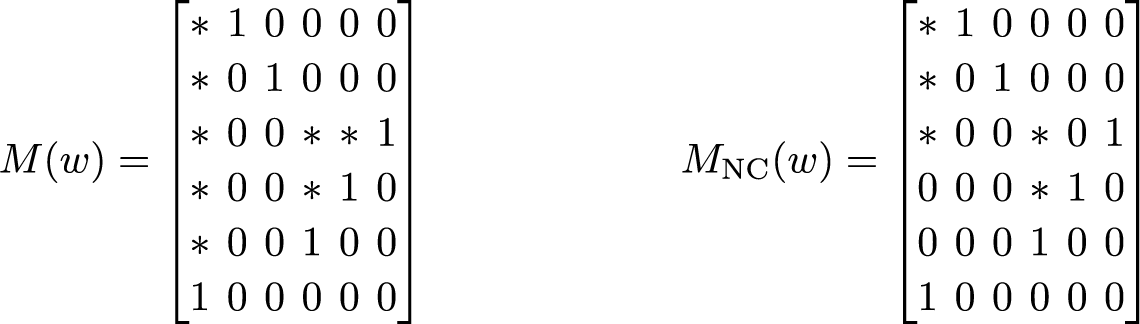
For
$w = \operatorname {ForToNC}(F)$
 , we have a canonical identification

See, for example, Figure 10. We now state the main result of the section.
Theorem 9.7. For
$w\in \operatorname {NC}_n$
 we have
$\mathrm {QFl}_n\cap BwB=M_{\operatorname {NC}}(w)B$
we have
$\mathrm {QFl}_n\cap BwB=M_{\operatorname {NC}}(w)B$
 and
and
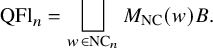
Moreover, for any total ordering
$w_1,w_2,\ldots ,w_{|\operatorname {NC}_{n}|}$
 of
$\operatorname {NC}_n$
of
$\operatorname {NC}_n$
 that extends the Bruhat order we set
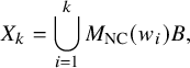
then each
$X_k$
 is closed,
$X_{1} \subseteq X_{2} \subseteq \cdots \subseteq X_{|\operatorname {NC}_{n}|} = \mathrm {QFl}_{n}$
is closed,
$X_{1} \subseteq X_{2} \subseteq \cdots \subseteq X_{|\operatorname {NC}_{n}|} = \mathrm {QFl}_{n}$
 , and
$X_{k+1}\setminus X_k=M_{\operatorname {NC}}(w_{k+1})B$
, and
$X_{k+1}\setminus X_k=M_{\operatorname {NC}}(w_{k+1})B$
 .
.
We will prove this result at the end of the section after some preparation.
Remark 9.8. The second part of Theorem 9.7 shows that the
$X_{i}$
 form an affine paving of
$\mathrm {QFl}_{n}$
form an affine paving of
$\mathrm {QFl}_{n}$
 ; see Section 11.1 for precise definitions.
Our first step is to extend a combinatorial characterization of the noncrossing inversion set stated in [Reference Bergeron, Gagnon, Nadeau, Spink and Tewari6, Remark 8.18]. For
$\widehat {F} \in \operatorname {BNestFor}_{n}$
 , the
$\color {blue}{{spread}}$
, the
$\color {blue}{{spread}}$
 of
$v \in \operatorname {IN}(\widehat {F})$
of
$v \in \operatorname {IN}(\widehat {F})$
 is the pair
$(i, j)$
is the pair
$(i, j)$
 consisting of the leftmost leaf descendant i of v and the rightmost leaf descendant j of v. Figure 11 depicts a bicolored nested forest in which each internal node is labeled by its spread. Note that the spread of an internal node v is not necessarily the transposition
$\tau _v$
consisting of the leftmost leaf descendant i of v and the rightmost leaf descendant j of v. Figure 11 depicts a bicolored nested forest in which each internal node is labeled by its spread. Note that the spread of an internal node v is not necessarily the transposition
$\tau _v$
 assigned to each
$v \in \operatorname {IN}(\widehat {F})$
assigned to each
$v \in \operatorname {IN}(\widehat {F})$
 earlier in Section 6.
A bicolored nested forest with spreads recorded for each internal node.
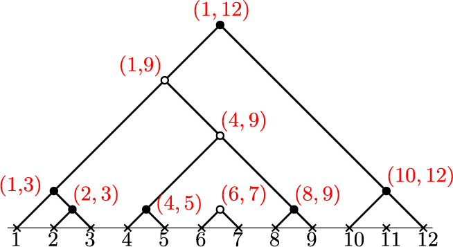
Figure 11 Long description
A tree diagram sits above a horizontal baseline marked with integers 1 through 12, each indicated by an x symbol. The tree consists of black filled nodes and white hollow nodes, each labeled with a red coordinate pair representing a spread.
At the top, the root node is a black dot labeled (1, 12). It branches left to a white node (1, 9) and right to a black node (10, 12).
From the white node (1, 9), the tree branches left to a black node (1, 3) and right to a white node (4, 9).
From the black node (1, 3), it branches to leaf nodes 1 and 2, with an intermediate black node (2, 3) branching to leaf nodes 2 and 3.
From the white node (4, 9), it branches left to a black node (4, 5) which connects to leaf nodes 4 and 5, and right to a black node (8, 9) which connects to leaf nodes 8 and 9. Between these, a white node (6, 7) connects to leaf nodes 6 and 7.
On the far right, the black node (10, 12) branches down to leaf nodes 10 and 12, with an intermediate connection to leaf node 11.
Proposition 9.9. If
$\widehat {F} \in \operatorname {BNestFor}^{\operatorname {nf}}_{n}$
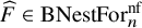 and
$w = \operatorname {ForToNC}(\widehat {F})$
and
$w = \operatorname {ForToNC}(\widehat {F})$
 , then

In particular, if
${F} \in \operatorname {\mathsf {Forest}}_{n}$
 , then
$\operatorname {Inv}_{\operatorname {NC}}(w)$
, then
$\operatorname {Inv}_{\operatorname {NC}}(w)$
 is the set of all spreads for
$v \in \operatorname {IN}({F})$
is the set of all spreads for
$v \in \operatorname {IN}({F})$
 .
.
Proof. By Proposition 8.10, it is sufficient to show that the set of elements of
$I_{\widehat {F}}$
 that are adjacent to w give the spreads of all black nodes in
$\widehat {F}$
that are adjacent to w give the spreads of all black nodes in
$\widehat {F}$
 . We do so using induction on n. As
$n = 1$
. We do so using induction on n. As
$n = 1$
 is vacuous, assume that
$n> 1$
is vacuous, assume that
$n> 1$
 and write
$\widehat {F} = \widehat {G} \cdot \mathsf {x}_{k}$
and write
$\widehat {F} = \widehat {G} \cdot \mathsf {x}_{k}$
 and
$u = \operatorname {ForToNC}(\widehat {G})$
and
$u = \operatorname {ForToNC}(\widehat {G})$
 with
$\widehat {G}\in \operatorname {BNestFor}^{\operatorname {nf}}_{n-1}$
with
$\widehat {G}\in \operatorname {BNestFor}^{\operatorname {nf}}_{n-1}$
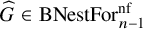 . We split into cases according to Lemma 8.9. First, suppose that either
$\mathsf {x}_{k}=\mathsf {r}_{k}^-$
. We split into cases according to Lemma 8.9. First, suppose that either
$\mathsf {x}_{k}=\mathsf {r}_{k}^-$
 or that leaf k is a right child of
$\widehat {G}$
or that leaf k is a right child of
$\widehat {G}$
 (so in particular
$\mathsf {x}_{k}\ne \mathsf {e}_{k}$
(so in particular
$\mathsf {x}_{k}\ne \mathsf {e}_{k}$
 ). Then for any
$v \in \operatorname {IN}(\widehat {G})$
). Then for any
$v \in \operatorname {IN}(\widehat {G})$
 with spread
$(i, j)$
with spread
$(i, j)$
 we have
$\Psi _{k}^{-}\big (u(i\, j)\big ) = w \Psi _{k}^{-}\big ((i\, j)\big )=w(i + \delta _{i \ge k}, j + \delta _{j \ge k})$
we have
$\Psi _{k}^{-}\big (u(i\, j)\big ) = w \Psi _{k}^{-}\big ((i\, j)\big )=w(i + \delta _{i \ge k}, j + \delta _{j \ge k})$
 , and the node in
$\operatorname {IN}(\widehat {F})$
, and the node in
$\operatorname {IN}(\widehat {F})$
 corresponding to v has spread
$(i + \delta _{i \ge k}, j + \delta _{j \ge k})$
corresponding to v has spread
$(i + \delta _{i \ge k}, j + \delta _{j \ge k})$
 so the claim holds.
Now suppose
$\mathsf {x}_{k}\ne \mathsf {r}_{k}^-$
 and k is not a right child in
$\widehat {G}$
and k is not a right child in
$\widehat {G}$
 . If
$\mathsf {x}_{k}=\mathsf {r}_{k}^+$
. If
$\mathsf {x}_{k}=\mathsf {r}_{k}^+$
 ,
$\Psi _k^+(u(ij))=ws_k(i+\delta _{i\ge k},j+\delta _{j\ge k})s_k=w(i+\delta _{i\ge k+1},j+\delta _{j\ge k+1})$
,
$\Psi _k^+(u(ij))=ws_k(i+\delta _{i\ge k},j+\delta _{j\ge k})s_k=w(i+\delta _{i\ge k+1},j+\delta _{j\ge k+1})$
 , and we conclude as before. If
$\mathsf {x}_{k} = \mathsf {e}_{k}$
, and we conclude as before. If
$\mathsf {x}_{k} = \mathsf {e}_{k}$
 then the same reasoning applies except that
$\widehat {F}$
then the same reasoning applies except that
$\widehat {F}$
 has one more black node than
$\widehat {G}$
has one more black node than
$\widehat {G}$
 , with spread
$(k, k+1)$
, with spread
$(k, k+1)$
 , and w has the additional adjacent element
$w s_{k}$
, and w has the additional adjacent element
$w s_{k}$
 .
.
We next give a recursive characterization of the charts in
$\mathrm {Fl}_{n}$
 determined by the
$M_{\operatorname {NC}}(F)$
determined by the
$M_{\operatorname {NC}}(F)$
 using the building operations from Section 3.
Proposition 9.10. The representatives of the noncrossing Bruhat cells in
$\mathrm {Fl}_{n}$
 are characterized recursively by
$M_{\operatorname {NC}}(\mathsf {r}_{1}^{-})B = \mathrm {Fl}_{1}$
are characterized recursively by
$M_{\operatorname {NC}}(\mathsf {r}_{1}^{-})B = \mathrm {Fl}_{1}$
 and for
$F = G \cdot \mathsf {e}_{i} \in \operatorname {\mathsf {Forest}}_{n}$
and for
$F = G \cdot \mathsf {e}_{i} \in \operatorname {\mathsf {Forest}}_{n}$
 ,
,

We prove the proposition using a technical argument involving a modified version of the
$\mathbb {G}_{i}$
 operation. Given a matrix M with column i equal to the jth basis vector for
$j < i$
operation. Given a matrix M with column i equal to the jth basis vector for
$j < i$
 , let
$\mathbb {G}_i'M$
, let
$\mathbb {G}_i'M$
 be obtained from
$\Psi _i^-M$
be obtained from
$\Psi _i^-M$
 by setting the
$j,i$
by setting the
$j,i$
 -entry to
$+$
-entry to
$+$
 .
.
Example 9.11. We have

Lemma 9.12. If M is an
$(m-1)\times (m-1)$
 matrix whose i-th column is
$e_j$
matrix whose i-th column is
$e_j$
 for some
$j<i$
for some
$j<i$
 , then we have an equality of sets
$(\mathbb {G}_iM)B_m=(\mathbb {G}_i'M)B_m$
, then we have an equality of sets
$(\mathbb {G}_iM)B_m=(\mathbb {G}_i'M)B_m$
 .
.
Proof. For
$x \in \mathbb C^{\times }$
 , let
$(\mathbb {G}_{i}M)(x)$
, let
$(\mathbb {G}_{i}M)(x)$
 and
$(\mathbb {G}_{i}'M)(x^{-1})$
and
$(\mathbb {G}_{i}'M)(x^{-1})$
 denote the matrices obtained by setting the newly introduced
$+$
denote the matrices obtained by setting the newly introduced
$+$
 ’s to x and
$x^{-1}$
’s to x and
$x^{-1}$
 , respectively. Let
$c_{i}$
, respectively. Let
$c_{i}$
 and
$c_{i+1}$
and
$c_{i+1}$
 be the i-th and
$i+1$
be the i-th and
$i+1$
 st columns of
$(\mathbb {G}_{i}M)(x)$
st columns of
$(\mathbb {G}_{i}M)(x)$
 . Then
$(\mathbb {G}_{i}'M)(x^{-1})$
. Then
$(\mathbb {G}_{i}'M)(x^{-1})$
 is obtained from
$(\mathbb {G}_{i}M)(x)$
is obtained from
$(\mathbb {G}_{i}M)(x)$
 by performing the column operations
$c_i \mapsto x^{-1}c_i$
by performing the column operations
$c_i \mapsto x^{-1}c_i$
 followed by
$c_{i+1} \mapsto x c_i -x c_{i+1}$
followed by
$c_{i+1} \mapsto x c_i -x c_{i+1}$
 . Both forward column operations correspond to right multiplication by elements of
$B_m$
. Both forward column operations correspond to right multiplication by elements of
$B_m$
 , so we have
$(\mathbb {G}_{i}M)(x)B_m = (\mathbb {G}_{i}'M)(x^{-1})B_m$
, so we have
$(\mathbb {G}_{i}M)(x)B_m = (\mathbb {G}_{i}'M)(x^{-1})B_m$
 . We conclude as
$x\mapsto x^{-1}$
. We conclude as
$x\mapsto x^{-1}$
 is a bijection on
$\mathbb {C}^\times $
is a bijection on
$\mathbb {C}^\times $
 .
.
Proof of Proposition 9.10
Let
$w = \operatorname {ForToNC}(F)$
 and
$u = \operatorname {ForToNC}(G)$
and
$u = \operatorname {ForToNC}(G)$
 . By Lemma 8.9, we have
$w = \Psi _{i}^{\pm }(u)$
. By Lemma 8.9, we have
$w = \Psi _{i}^{\pm }(u)$
 . Further, by Proposition 9.9, we have

Thus, if we write
$M_{\operatorname {NC}}(w; x)$
 for the matrix obtained from
$M_{\operatorname {NC}}(w)$
for the matrix obtained from
$M_{\operatorname {NC}}(w)$
 by setting the
$(w(i+1), i)$
by setting the
$(w(i+1), i)$
 entry equal to x, then we have

Moreover,
$M_{\operatorname {NC}}(w) = M_{\operatorname {NC}}(w; 0) \sqcup M_{\operatorname {NC}}(w; +)$
 , so we complete the proof by showing that

If leaf i is not a right child in G, then
$w(i)> w(i+1)$
 and we have a direct equality
$M_{\operatorname {NC}}(w; +) = \mathbb {G}_{i}M_{\operatorname {NC}}(u)$
and we have a direct equality
$M_{\operatorname {NC}}(w; +) = \mathbb {G}_{i}M_{\operatorname {NC}}(u)$
 . If leaf i is a right child in G, then
$w(i) < w(i+1)$
. If leaf i is a right child in G, then
$w(i) < w(i+1)$
 and
$M_{\operatorname {NC}}(w; +) = \mathbb {G}_{i}'M_{\operatorname {NC}}(u)$
and
$M_{\operatorname {NC}}(w; +) = \mathbb {G}_{i}'M_{\operatorname {NC}}(u)$
 , so we must use Lemma 9.12 to relate
$\mathbb {G}_{i}'$
, so we must use Lemma 9.12 to relate
$\mathbb {G}_{i}'$
 and
$\mathbb {G}_{i}$
and
$\mathbb {G}_{i}$
 . Indeed, as a right child i can never be the left endpoint of an internal node, Proposition 9.9 implies that u has no noncrossing inversion ending in i. Thus
$M_{\operatorname {NC}}(G)$
. Indeed, as a right child i can never be the left endpoint of an internal node, Proposition 9.9 implies that u has no noncrossing inversion ending in i. Thus
$M_{\operatorname {NC}}(G)$
 has no
$\ast $
has no
$\ast $
 ’s in column i and the hypotheses of Lemma 9.12 are satisfied, giving
$M_{\operatorname {NC}}(w; +)B = \mathbb {G}_{i}M_{\operatorname {NC}}(u)B$
’s in column i and the hypotheses of Lemma 9.12 are satisfied, giving
$M_{\operatorname {NC}}(w; +)B = \mathbb {G}_{i}M_{\operatorname {NC}}(u)B$
 .
.
Proposition 9.13. Let
$w \in \operatorname {NC}_{n}$
 , and let F be the unique forest in
$\operatorname {\mathsf {Forest}}_n$
, and let F be the unique forest in
$\operatorname {\mathsf {Forest}}_n$
 such that
$w=\operatorname {ForToNC}(F)$
such that
$w=\operatorname {ForToNC}(F)$
 . We have
$M_{\operatorname {NC}}(F)B = C(F)$
. We have
$M_{\operatorname {NC}}(F)B = C(F)$
 , and as a consequence there is a T-equivariant isomorphism

Proof. We show that
$C(F)$
 agrees with the recursive characterization of
$M_{\operatorname {NC}}(F)B$
agrees with the recursive characterization of
$M_{\operatorname {NC}}(F)B$
 given in Proposition 9.10. As
$C((\mathsf {r}_{1}^{-})^{n-k}) = \operatorname {id}_{S_{n-k}}\in \mathrm {Fl}_{n-k}$
given in Proposition 9.10. As
$C((\mathsf {r}_{1}^{-})^{n-k}) = \operatorname {id}_{S_{n-k}}\in \mathrm {Fl}_{n-k}$
 , this amounts to showing that for
$F = G \cdot \mathsf {e}_{i} \in \operatorname {\mathsf {Forest}}_{n}$
, this amounts to showing that for
$F = G \cdot \mathsf {e}_{i} \in \operatorname {\mathsf {Forest}}_{n}$
 ,
,

By the definition of
$\mathrm {Face}(\widehat {F})$
 and the
$\le _{re}$
and the
$\le _{re}$
 order, we have

If we furthermore write
$w = \operatorname {ForToNC}(F)$
 and
$u = \operatorname {ForToNC}(G)$
and
$u = \operatorname {ForToNC}(G)$
 , then by Lemma 8.9 we have
$w = \Psi ^{\epsilon }_{i}(u)$
, then by Lemma 8.9 we have
$w = \Psi ^{\epsilon }_{i}(u)$
 for
$\epsilon \in \{+, -\}$
for
$\epsilon \in \{+, -\}$
 . Thus

By intersecting the sets above, we arrive at the following description of
$C(F)$
 :
:
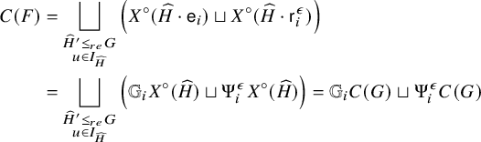
This completes the proof, as by Lemma 8.9
$\epsilon = -$
 if leaf i is a left child and
$+$
if leaf i is a left child and
$+$
 otherwise.
We can now complete the proof of Theorem 9.7.
Proof of Theorem 9.7
By Theorem 9.1,
$\mathrm {QFl}_{n}$
 is the disjoint union of the charts
$C(F)$
is the disjoint union of the charts
$C(F)$
 for
$F \in \operatorname {\mathsf {Forest}}_{n}$
for
$F \in \operatorname {\mathsf {Forest}}_{n}$
 . By Proposition 9.13, these charts are exactly the
$M_{\operatorname {NC}}(w)B$
. By Proposition 9.13, these charts are exactly the
$M_{\operatorname {NC}}(w)B$
 for
$w\in \operatorname {NC}_n$
for
$w\in \operatorname {NC}_n$
 , giving Equation (9.6). As
$M_{\operatorname {NC}}(w)B \subseteq M(w)B=BwB$
, giving Equation (9.6). As
$M_{\operatorname {NC}}(w)B \subseteq M(w)B=BwB$
 , and the
$B w B$
, and the
$B w B$
 form a partition of
$\mathrm {Fl}_{n}$
form a partition of
$\mathrm {Fl}_{n}$
 by (2.1), it follows that
$M_{\operatorname {NC}}(w)B = \mathrm {QFl}_n\cap M(w)B$
by (2.1), it follows that
$M_{\operatorname {NC}}(w)B = \mathrm {QFl}_n\cap M(w)B$
 .
.
Now for any
$w\in S_n$
 , the Schubert variety
$X^{w} = \overline {BwB}$
, the Schubert variety
$X^{w} = \overline {BwB}$
 consists of all
$BuB$
consists of all
$BuB$
 with
$u \le w$
with
$u \le w$
 in Bruhat order. It follows that
$X_{k} = \mathrm {QFl}_n\cap \big ( \bigcup _{i=1}^{k} X^{w_{i}} \big )$
in Bruhat order. It follows that
$X_{k} = \mathrm {QFl}_n\cap \big ( \bigcup _{i=1}^{k} X^{w_{i}} \big )$
 is closed, which concludes the proof.
10 Intrinsic characterizations of
$\mathrm {QFl}_n$

We now give two intrinsic characterizations of
$\mathrm {QFl}_n$
 . These characterizations are independent of one another and are presented in Sections 10.1 and 10.2.
10.1 Characterization with Plücker functions
This section proves Theorem B, which states that
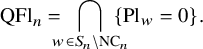
The proof is given at the end of the section. We begin with a classical observation, which can be found for instance in [Reference Lee, Masuda and Park35, Proposition 2.6].
Proposition 10.1. For
$\mathcal {F} \in \mathrm {Fl}_{n}$
 , the set of torus fixed points in
$\overline {T \cdot \mathcal {F}}$
, the set of torus fixed points in
$\overline {T \cdot \mathcal {F}}$
 is
$\{wB \;|\; \mathrm {Pl}_{w}(\mathcal {F}) \neq 0\}$
is
$\{wB \;|\; \mathrm {Pl}_{w}(\mathcal {F}) \neq 0\}$
 .
.
Every element of
$BwB$
 has a unique representative h in the set
$M(w)$
has a unique representative h in the set
$M(w)$
 defined in Section 9. Thus when restricted to
$BwB$
defined in Section 9. Thus when restricted to
$BwB$
 , we can view the Plücker functions as polynomials in the matrix entries which are not uniformly
$0$
, we can view the Plücker functions as polynomials in the matrix entries which are not uniformly
$0$
 or
$1$
or
$1$
 across all of
$M(w)$
across all of
$M(w)$
 , namely the
$h_{w(j), i}$
, namely the
$h_{w(j), i}$
 for
$(i, j) \in \operatorname {Inv}(w)$
for
$(i, j) \in \operatorname {Inv}(w)$
 . Going forward, we define a
$\mathbb Z^{n}$
. Going forward, we define a
$\mathbb Z^{n}$
 -grading on such polynomials by setting

where
$e_{k}$
 denotes the kth standard basis vector. This grading is the weight of the character of the T-action on each entry of
$M(w)$
denotes the kth standard basis vector. This grading is the weight of the character of the T-action on each entry of
$M(w)$
 under the action of T as described in Section 9.
Observation 10.2. Let
$w \in S_{n}$
 . Expressed in the entries of
$h \in M(w)$
. Expressed in the entries of
$h \in M(w)$
 ,
$\mathrm {Pl}_{u}(h)/\mathrm {Pl}_{w}(h)$
,
$\mathrm {Pl}_{u}(h)/\mathrm {Pl}_{w}(h)$
 is a homogeneous polynomial of degree
$\sum (u^{-1}(i)-w^{-1}(i))e_{n+1-i}$
is a homogeneous polynomial of degree
$\sum (u^{-1}(i)-w^{-1}(i))e_{n+1-i}$
 for each
$u \in S_{n}$
for each
$u \in S_{n}$
 .
.
Proof. We compute directly that
$\mathrm {Pl}_{w}(h) = 1$
 , so
$\mathrm {Pl}_{u}(h)/\mathrm {Pl}_{w}(h) = \mathrm {Pl}_{u}(h)$
, so
$\mathrm {Pl}_{u}(h)/\mathrm {Pl}_{w}(h) = \mathrm {Pl}_{u}(h)$
 has denominator
$1$
has denominator
$1$
 . The claim now follows from the fact that the Plücker functions are T-equivariant and the weight of the character by which T scales
$\mathrm {Pl}_{u}(h)/\mathrm {Pl}_{w}(h)$
. The claim now follows from the fact that the Plücker functions are T-equivariant and the weight of the character by which T scales
$\mathrm {Pl}_{u}(h)/\mathrm {Pl}_{w}(h)$
 is
$\sum u^{-1}(i)e_{n+1-i} - \sum w^{-1}(i)e_{n+1-i}$
is
$\sum u^{-1}(i)e_{n+1-i} - \sum w^{-1}(i)e_{n+1-i}$
 .
.
In order to perform a more granular analysis on the degree of each Plücker function, we establish some notation using the root system of type
$A_{n-1}$
 . The positive roots in this system are the vectors
$e_{i} - e_{j}$
. The positive roots in this system are the vectors
$e_{i} - e_{j}$
 for
$1 \le i < j \le n$
for
$1 \le i < j \le n$
 and the negative roots are
$e_{j} - e_{i}$
and the negative roots are
$e_{j} - e_{i}$
 for
$1 \le i < j \le n$
for
$1 \le i < j \le n$
 . Given
$F\in \operatorname {\mathsf {Forest}}_{n}$
. Given
$F\in \operatorname {\mathsf {Forest}}_{n}$
 , we define the polyhedral cone
$\operatorname {Cone}_{F}$
, we define the polyhedral cone
$\operatorname {Cone}_{F}$
 by
by

and for
$w\in \operatorname {NC}_n$
 we define
$\operatorname {Cone}_{w}= w \cdot \operatorname {Cone}_{F}$
we define
$\operatorname {Cone}_{w}= w \cdot \operatorname {Cone}_{F}$
 where
$F\in \operatorname {\mathsf {Forest}}_n$
where
$F\in \operatorname {\mathsf {Forest}}_n$
 is the unique forest such that
$w=\operatorname {ForToNC}(F)$
is the unique forest such that
$w=\operatorname {ForToNC}(F)$
 . In view of Proposition 9.9

Spreads are characterized by the fact that if
$(i, j)$
 is a spread in
$F \in \operatorname {\mathsf {Forest}}_{n}$
is a spread in
$F \in \operatorname {\mathsf {Forest}}_{n}$
 , then no spread has the form
$(j, k)$
, then no spread has the form
$(j, k)$
 . Such sets (and their associated cones) were first studied in [Reference Gelfand, Graev and Postnikov23] and are commonly known as
$\color {blue}{{noncrossing\, alternating\, forests}}$
. Such sets (and their associated cones) were first studied in [Reference Gelfand, Graev and Postnikov23] and are commonly known as
$\color {blue}{{noncrossing\, alternating\, forests}}$
 ; see, for example, [Reference Albenque and Nadeau1]. The following result can be found in [Reference Gelfand, Graev and Postnikov23, §6].
Proposition 10.3. For each
$w \in \operatorname {NC}_{n}$
 ,
$\operatorname {Cone}_{w}$
,
$\operatorname {Cone}_{w}$
 is simplicial and the only roots it contains are the generators
$e_{w(j)} - e_{w(i)}$
is simplicial and the only roots it contains are the generators
$e_{w(j)} - e_{w(i)}$
 for
$(i,j)\in \operatorname {Inv}_{\operatorname {NC}}(w)$
for
$(i,j)\in \operatorname {Inv}_{\operatorname {NC}}(w)$
 .
.
The sets
$(w(b), w(a))$
 for
$(a, b)$
for
$(a, b)$
 a spread in F also appear in the literature as a generalization of noncrossing alternating forests. Specifically, [Reference Josuat-Vergès and Nadeau31, §6] shows that these are canonically in bijection with the set of
$\boldsymbol {c}$
a spread in F also appear in the literature as a generalization of noncrossing alternating forests. Specifically, [Reference Josuat-Vergès and Nadeau31, §6] shows that these are canonically in bijection with the set of
$\boldsymbol {c}$
 -clusters.
Proof of Theorem B
First, we take
$\mathcal {F}\in \mathrm {QFl}_n$
 . By Theorem 6.1, the torus fixed points in
$\overline {T \cdot \mathcal {F}}$
. By Theorem 6.1, the torus fixed points in
$\overline {T \cdot \mathcal {F}}$
 are all noncrossing partitions. By Proposition 10.1, this means that the nonvanishing Plücker functions of
$\mathcal {F}$
are all noncrossing partitions. By Proposition 10.1, this means that the nonvanishing Plücker functions of
$\mathcal {F}$
 are also indexed by elements of
$\operatorname {NC}_{n}$
are also indexed by elements of
$\operatorname {NC}_{n}$
 .
.
Conversely, suppose that
$\mathrm {Pl}_{u}\mathcal {F} = 0$
 for all
$u\in S_n\setminus \operatorname {NC}_n$
for all
$u\in S_n\setminus \operatorname {NC}_n$
 . Let
$w\in S_n$
. Let
$w\in S_n$
 be such that
$\mathcal {F}\in BwB$
be such that
$\mathcal {F}\in BwB$
 and let
$h \in \mathrm {GL}_n$
and let
$h \in \mathrm {GL}_n$
 be the representative of
$\mathcal {F}$
be the representative of
$\mathcal {F}$
 in
$M(w)$
in
$M(w)$
 . As
$\mathrm {Pl}_w\mathcal {F}\ne 0$
. As
$\mathrm {Pl}_w\mathcal {F}\ne 0$
 on
$BwB$
on
$BwB$
 we conclude that
$w\in \operatorname {NC}_n$
we conclude that
$w\in \operatorname {NC}_n$
 . We now claim that for each
$(a, b)\in \operatorname {Inv}(w)\setminus \operatorname {Inv}_{\operatorname {NC}}(w)$
. We now claim that for each
$(a, b)\in \operatorname {Inv}(w)\setminus \operatorname {Inv}_{\operatorname {NC}}(w)$
 we have
$h_{w(b),a}=0$
we have
$h_{w(b),a}=0$
 .
.
We proceed by induction on
$w(a) - w(b)$
 . Let
$u = w(a\,b)$
. Let
$u = w(a\,b)$
 and let
$\alpha = (b-a)(e_{w(b)} - e_{w(a)})$
and let
$\alpha = (b-a)(e_{w(b)} - e_{w(a)})$
 . We consider the set S consisting of all multisubsets M of
$\operatorname {Inv}(w)$
. We consider the set S consisting of all multisubsets M of
$\operatorname {Inv}(w)$
 with the property that
$\sum _{(i, j) \in M} e_{w(j)} - e_{w(i)} = \alpha $
with the property that
$\sum _{(i, j) \in M} e_{w(j)} - e_{w(i)} = \alpha $
 so that by Observation 10.2 we have

We now describe some properties of the elements
$M \in S$
 . First, by considering the first and last nonzero coordinate in the sum
$\sum _{(i, j) \in M} e_{w(j)} - e_{w(i)} = \alpha $
. First, by considering the first and last nonzero coordinate in the sum
$\sum _{(i, j) \in M} e_{w(j)} - e_{w(i)} = \alpha $
 , every
$e_{w(j)} - e_{w(i)} \in M$
, every
$e_{w(j)} - e_{w(i)} \in M$
 has either
$w(j) - w(i) < w(b) - w(a)$
has either
$w(j) - w(i) < w(b) - w(a)$
 or
$(i, j) = (a, b)$
or
$(i, j) = (a, b)$
 . Second, by Proposition 10.3, M must contain at least one element of the form
$e_{w(j)} - e_{w(i)}$
. Second, by Proposition 10.3, M must contain at least one element of the form
$e_{w(j)} - e_{w(i)}$
 for
$(i, j) \in \operatorname {Inv}(w)\setminus \operatorname {Inv}_{\operatorname {NC}}(w)$
for
$(i, j) \in \operatorname {Inv}(w)\setminus \operatorname {Inv}_{\operatorname {NC}}(w)$
 . Finally, a direct computation of
$\mathrm {Pl}_{u}(h)/\mathrm {Pl}_{w}(h)$
. Finally, a direct computation of
$\mathrm {Pl}_{u}(h)/\mathrm {Pl}_{w}(h)$
 shows that the coefficient of
$(h_{w(b), a})^{b-a}$
shows that the coefficient of
$(h_{w(b), a})^{b-a}$
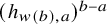 is nonzero: for
$i < a$
is nonzero: for
$i < a$
 or
$i \ge b$
or
$i \ge b$
 ,
$\det (h_{u(1), \ldots , u(i)}) = \det (h_{w(1), \ldots , w(i)}) = \pm 1$
,
$\det (h_{u(1), \ldots , u(i)}) = \det (h_{w(1), \ldots , w(i)}) = \pm 1$
 , while for
$a \le i < b$
, while for
$a \le i < b$
 ,
$\det (h_{u(1), \ldots , u(i)})$
,
$\det (h_{u(1), \ldots , u(i)})$
 contains
$h_{w(b), a}$
contains
$h_{w(b), a}$
 with a coefficient of
$\pm 1$
with a coefficient of
$\pm 1$
 . Thus by our assumption on
$\mathrm {Pl}_{u}$
. Thus by our assumption on
$\mathrm {Pl}_{u}$
 and our inductive hypothesis, we have
$0 = (h_{w(b), a})^{b-a}$
and our inductive hypothesis, we have
$0 = (h_{w(b), a})^{b-a}$
 . This proves the claim. This shows
$h\in M_{\operatorname {NC}}(w)$
. This proves the claim. This shows
$h\in M_{\operatorname {NC}}(w)$
 and finally
$\mathcal {F}\in \mathrm {QFl}_n$
and finally
$\mathcal {F}\in \mathrm {QFl}_n$
 by Proposition 9.13.
10.2 Characterization via equivalence of flags
We now give our second characterization of
$\mathrm {QFl}_{n}$
 as flags that can be obtained from
$\mathrm {id}_{\mathrm {Fl}_{n}}$
as flags that can be obtained from
$\mathrm {id}_{\mathrm {Fl}_{n}}$
 , the standard coordinate flag
$\{0\}\subset \{e_1\}\subset \{e_1,e_2\}\subset \cdots \subset \{e_1,\dots ,e_n\}$
, the standard coordinate flag
$\{0\}\subset \{e_1\}\subset \{e_1,e_2\}\subset \cdots \subset \{e_1,\dots ,e_n\}$
 , via certain elementary operations.
Definition 10.4. Define
$\sim $
 to be the equivalence relation on complete flags generated by the relations
$\sim _i$
to be the equivalence relation on complete flags generated by the relations
$\sim _i$
 for
$1\le i \le n-1$
for
$1\le i \le n-1$
 given by
$\mathcal {F}\sim _i \mathcal {G}$
given by
$\mathcal {F}\sim _i \mathcal {G}$
 if
if
-
(1) $\mathcal {F}_j=\mathcal {G}_{j}$
for all
$j\ne i$
, and -
(2) $e_i\in \mathcal {F}_{i+1}$
and
$\mathcal {F}_{i-1}\subset \{x_i=0\}$
.



We have that
$\mathcal {F}\sim _i \mathcal {G}$
 for
$1\leq i\leq n-1$
for
$1\leq i\leq n-1$
 if and only if there exists
$\mathcal {H}\in \mathrm {Fl}_{n-1}$
if and only if there exists
$\mathcal {H}\in \mathrm {Fl}_{n-1}$
 such that
$\mathcal {F},\mathcal {G}\in \mathbb {P}_{i}\mathcal {H}$
such that
$\mathcal {F},\mathcal {G}\in \mathbb {P}_{i}\mathcal {H}$
 , where
$\mathbb {P}_{i}$
, where
$\mathbb {P}_{i}$
 is defined in Section 3.2. In particular, note that
$\Psi _i^{-}\mathcal {H}\sim _i \Psi _i^{+}\mathcal {H}$
is defined in Section 3.2. In particular, note that
$\Psi _i^{-}\mathcal {H}\sim _i \Psi _i^{+}\mathcal {H}$
 .
.
Theorem 10.5. The quasisymmetric flag variety
$\mathrm {QFl}_n\subset \mathrm {Fl}_{n}$
 is the equivalence class of
$\sim $
is the equivalence class of
$\sim $
 containing the standard coordinate flag.
We prove this at the end of the subsection after a preparatory lemma.
Lemma 10.6. Let
$\widehat {F}\in \operatorname {BNestFor}_n$
 . Suppose there exists i such that every element
$w\in I_{\widehat {F}}$
. Suppose there exists i such that every element
$w\in I_{\widehat {F}}$
 satisfies
$i\in \{w(i),w(i+1)\}$
satisfies
$i\in \{w(i),w(i+1)\}$
 . Then we have
$X(\widehat {F})\subset \mathbb {P}_{i}X(\widehat {G})$
. Then we have
$X(\widehat {F})\subset \mathbb {P}_{i}X(\widehat {G})$
 for some
$\widehat {G}\in \operatorname {BNestFor}_{n-1}$
for some
$\widehat {G}\in \operatorname {BNestFor}_{n-1}$
 .
.
Proof. We will prove the following statements, from which the conclusion follows immediately.
-
(i) If $w(i)=i$
for all
$w\in I_{\widehat {F}}$
, then
$\widehat {F}=\widehat {G} \cdot \mathsf {r}_{i}^-$
for some
$\widehat {G} \in \operatorname {BNestFor}_{n-1}$
. -
(ii) If $w(i+1)=i$
for all
$w\in I_{\widehat {F}}$
, then
$\widehat {F}\overset {c}{\sim } \widehat {G}\cdot \mathsf {r}_{i}^+$
for some
$\widehat {G} \in \operatorname {BNestFor}_{n-1}$
. -
(iii) If $i\in \{w(i),w(i+1)\}$
for all
$w\in I_{\widehat {F}}$
, but we are not in a scenario covered by Cases (i) and (ii), then
$\widehat {F}\overset {c}{\sim } \widehat {G}\cdot \mathsf {e}_{i}$
for some
$\widehat {G} \in \operatorname {BNestFor}_{n-1}$
.










If we are in case (i), then
$\operatorname {NCPerm}(\widehat {F})\in I_{\widehat {F}}$
 has i as a fixed point, implying that the leaf labeled i is a singleton tree in
$\widehat {F}$
has i as a fixed point, implying that the leaf labeled i is a singleton tree in
$\widehat {F}$
 . This immediately yields
$\widehat {F}=\widehat {G}\cdot \mathsf {r}_{i}^-$
. This immediately yields
$\widehat {F}=\widehat {G}\cdot \mathsf {r}_{i}^-$
 .
.
Now suppose we are in a situation described in (ii). Let
$v\in \operatorname {IN}(\widehat {F})$
 have canonical label i. Let
$P_1$
have canonical label i. Let
$P_1$
 (respectively
$P_2$
(respectively
$P_2$
 ) be the path beginning from the leaf labeled i (respectively
$i+1$
) be the path beginning from the leaf labeled i (respectively
$i+1$
 ) and terminating in v. Observe that all but the final edge in
$P_1$
) and terminating in v. Observe that all but the final edge in
$P_1$
 connect a right child to its parent node and similarly all edges but the final edge in
$P_{2}$
connect a right child to its parent node and similarly all edges but the final edge in
$P_{2}$
 connect a left child to its parent. We claim that v must be white. Indeed, if v were black, then left edge deletion at v would result in an element in
$I_{\widehat {F}}$
connect a left child to its parent. We claim that v must be white. Indeed, if v were black, then left edge deletion at v would result in an element in
$I_{\widehat {F}}$
 that has i and
$i+1$
that has i and
$i+1$
 in different cycles. For similar reasons we infer that all nodes in
$P_2$
in different cycles. For similar reasons we infer that all nodes in
$P_2$
 are necessarily white. Thus we are in a situation depicted on the left in Figure 12 where the “half-filled” nodes could be black or white. By performing colored Tamari rotation as in Definition 8.3, first along
$P_1$
are necessarily white. Thus we are in a situation depicted on the left in Figure 12 where the “half-filled” nodes could be black or white. By performing colored Tamari rotation as in Definition 8.3, first along
$P_1$
 and then along
$P_2$
and then along
$P_2$
 as in Figure 12, one can obtain a bicolored nested forest wherein v has left and right children being leaves with labels i and
$i+1$
as in Figure 12, one can obtain a bicolored nested forest wherein v has left and right children being leaves with labels i and
$i+1$
 . Then as described in Definition 4.2, there exists a
$\widehat {G} \in \operatorname {BNestFor}_{n-1}$
. Then as described in Definition 4.2, there exists a
$\widehat {G} \in \operatorname {BNestFor}_{n-1}$
 satisfying
$\widehat {F}=\widehat {G}\cdot \mathsf {r}_{i}^+$
satisfying
$\widehat {F}=\widehat {G}\cdot \mathsf {r}_{i}^+$
 .
.
Case (ii) (left) and a bicolored nested forest that is colored Tamari equivalent. The half-filled nodes could be either black or white.
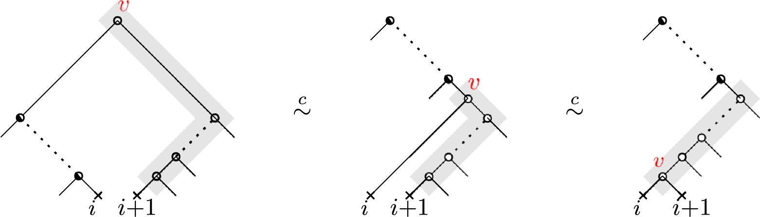
Finally we consider (iii). Let
$v\in \operatorname {IN}(\widehat {F})$
 have canonical label i, like before. For the condition in (iii) to hold, v must be black. Indeed, if v were white, then no element of
$I_{\widehat {F}}$
have canonical label i, like before. For the condition in (iii) to hold, v must be black. Indeed, if v were white, then no element of
$I_{\widehat {F}}$
 has i as a fixed point. For this same reason the left child of v is necessarily the leaf labeled i. As above, the path from the leaf labeled
$i+1$
has i as a fixed point. For this same reason the left child of v is necessarily the leaf labeled i. As above, the path from the leaf labeled
$i+1$
 to v can only contain white nodes, as this ensures that i and
$i+1$
to v can only contain white nodes, as this ensures that i and
$i+1$
 are in the same cycle if i is not a fixed point. We use colored Tamari rotations exactly as in Case (ii) to obtain a bicolored nested forest where v has left and right children given by i and
$i+1$
are in the same cycle if i is not a fixed point. We use colored Tamari rotations exactly as in Case (ii) to obtain a bicolored nested forest where v has left and right children given by i and
$i+1$
 . Left edge deletion at v now gives
$\widehat {G}\in \operatorname {BNestFor}_{n-1}$
. Left edge deletion at v now gives
$\widehat {G}\in \operatorname {BNestFor}_{n-1}$
 satisfying
$\widehat {F}=\widehat {G}\cdot \mathsf {e}_{i}$
satisfying
$\widehat {F}=\widehat {G}\cdot \mathsf {e}_{i}$
 . Figure 13 outlines this case.
Case (iii) (left) and a bicolored nested forest that is colored Tamari equivalent.
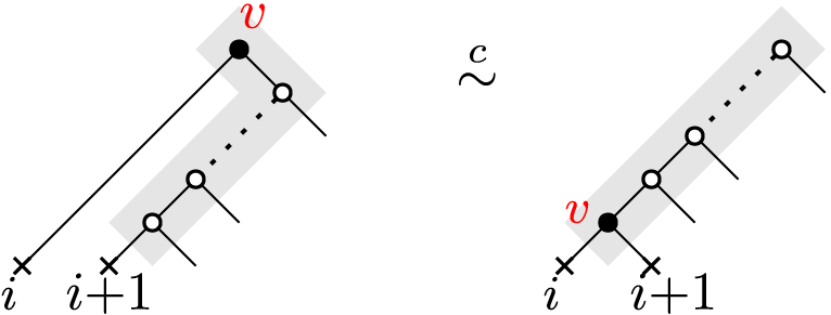
Proof of Theorem 10.5
First, we show that
$\mathrm {QFl}_n$
 is closed under these relations. Suppose first that
$\mathcal {F}\in \mathrm {QFl}_{n}$
is closed under these relations. Suppose first that
$\mathcal {F}\in \mathrm {QFl}_{n}$
 satisfies condition (2) in Definition 10.4 for a fixed i, which means that
$\mathcal {F}\in \mathbb {P}_i\mathrm {Fl}_{n-1}$
satisfies condition (2) in Definition 10.4 for a fixed i, which means that
$\mathcal {F}\in \mathbb {P}_i\mathrm {Fl}_{n-1}$
 .
.
We claim that in that case
$\mathcal {F}\in \mathbb {P}_i\mathrm {QFl}_{n-1}$
 . Condition (2) is closed and invariant under the action of T, so it is satisfied by all elements of the torus-orbit closure
$\overline {T \cdot \mathcal {F}}$
. Condition (2) is closed and invariant under the action of T, so it is satisfied by all elements of the torus-orbit closure
$\overline {T \cdot \mathcal {F}}$
 . By Theorem 5.1,
$\overline {T \cdot \mathcal {F}}=X(\widehat {F})$
. By Theorem 5.1,
$\overline {T \cdot \mathcal {F}}=X(\widehat {F})$
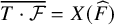 for some
$\widehat {F} \in \operatorname {BNestFor}_{n}$
for some
$\widehat {F} \in \operatorname {BNestFor}_{n}$
 , so the conditions (2) also apply to the set of torus fixed points
$I_{\widehat {F}}\subset \operatorname {NC}_n$
, so the conditions (2) also apply to the set of torus fixed points
$I_{\widehat {F}}\subset \operatorname {NC}_n$
 . This means that i is a fixed point or
$i,i+1$
. This means that i is a fixed point or
$i,i+1$
 are in the same cycle for each element of
$I_{\widehat {F}}$
are in the same cycle for each element of
$I_{\widehat {F}}$
 , so Lemma 10.6 guarantees the existence of
$\widehat {G} \in \operatorname {BNestFor}_{n-1}$
, so Lemma 10.6 guarantees the existence of
$\widehat {G} \in \operatorname {BNestFor}_{n-1}$
 such that
$X(\widehat {F})\subset \mathbb {P}_{i}X(\widehat {G})$
such that
$X(\widehat {F})\subset \mathbb {P}_{i}X(\widehat {G})$
 . This proves the claim since
$\mathcal {F} \in X(\widehat {F})$
. This proves the claim since
$\mathcal {F} \in X(\widehat {F})$
 and
$X(\widehat {G})\subset \mathrm {QFl}_{n-1}$
and
$X(\widehat {G})\subset \mathrm {QFl}_{n-1}$
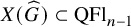 .
.
Now if
$\mathcal {F}\sim _i\mathcal {H}$
 , then by condition (1) we get
$\mathcal {H}\in \mathbb {P}_iX(\widehat {G})\subset \mathbb {P}_i\mathrm {QFl}_{n-1}$
, then by condition (1) we get
$\mathcal {H}\in \mathbb {P}_iX(\widehat {G})\subset \mathbb {P}_i\mathrm {QFl}_{n-1}$
 as well, and thus
$\mathcal {H}\in \mathrm {QFl}_{n}$
as well, and thus
$\mathcal {H}\in \mathrm {QFl}_{n}$
 .
.
Conversely, we now show that we can reduce every element of
$\mathrm {QFl}_n$
 to
$\operatorname {id}_{\mathrm {Fl}_{n}}$
to
$\operatorname {id}_{\mathrm {Fl}_{n}}$
 using these relations. We do this by induction on n, the case
$n=2$
using these relations. We do this by induction on n, the case
$n=2$
 being trivial.
Let
$\mathcal {F}\in \mathrm {QFl}_n$
 . Since
$\mathrm {QFl}_n=\mathbb {P}_1\mathrm {QFl}_{n-1}\cup \cdots \cup \mathbb {P}_{n-1}\mathrm {QFl}_{n-1}$
. Since
$\mathrm {QFl}_n=\mathbb {P}_1\mathrm {QFl}_{n-1}\cup \cdots \cup \mathbb {P}_{n-1}\mathrm {QFl}_{n-1}$
 and every element of
$\mathbb {P}_i\mathcal {H}$
and every element of
$\mathbb {P}_i\mathcal {H}$
 is
$\sim _i$
is
$\sim _i$
 -equivalent to
$\Psi _i^-\mathcal {H}$
-equivalent to
$\Psi _i^-\mathcal {H}$
 , there exist
$j\in \{1,\ldots ,n-1\}$
, there exist
$j\in \{1,\ldots ,n-1\}$
 and
$\mathcal {G}\in \mathrm {QFl}_{n-1}$
and
$\mathcal {G}\in \mathrm {QFl}_{n-1}$
 such that
$\mathcal {F}\sim _j\Psi _j^-\mathcal {G}$
such that
$\mathcal {F}\sim _j\Psi _j^-\mathcal {G}$
 . By the inductive hypothesis we know that
$\mathcal {G}\sim \operatorname {id}_{\mathrm {Fl}_{n-1}}$
. By the inductive hypothesis we know that
$\mathcal {G}\sim \operatorname {id}_{\mathrm {Fl}_{n-1}}$
 .
.
We claim that for any i,
$\mathcal {H}\sim _i \mathcal {H}'$
 in
$\mathrm {QFl}_{n-1}$
in
$\mathrm {QFl}_{n-1}$
 implies
$\Psi _j^-\mathcal {H}\sim \Psi _j^-\mathcal {H}'$
implies
$\Psi _j^-\mathcal {H}\sim \Psi _j^-\mathcal {H}'$
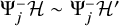 in
$\mathrm {QFl}_n$
in
$\mathrm {QFl}_n$
 . To prove this, we let
$\mathcal {K}\in \mathrm {QFl}_{n-2}$
. To prove this, we let
$\mathcal {K}\in \mathrm {QFl}_{n-2}$
 be such that
$\mathcal {H},\mathcal {H}'\in \mathbb {P}_i\mathcal {K}$
be such that
$\mathcal {H},\mathcal {H}'\in \mathbb {P}_i\mathcal {K}$
 and consider different cases.
-
(i) If $i\ge j$
, then by Lemma 4.6 we have
$\Psi _j^-\mathbb {P}_i\mathcal {K}=\mathbb {P}_{i+1}\Psi _{j}^-\mathcal {K}$
and so
$\Psi _j^-\mathcal {H}\sim _{i+1}\Psi _j^-\mathcal {H}'$
. -
(ii) If $j\ge i+2$
, then by Lemma 4.6 we have
$\Psi _j^-\mathbb {P}_i\mathcal {K}=\mathbb {P}_i\Psi _{j-1}^-\mathcal {K}$
and so
$\Psi _j^-\mathcal {H}\sim _i\Psi _j^-\mathcal {H}'$
. -
(iii) Finally, suppose $j=i+1$
. By Lemma 8.2 we have
$\Psi _{i+1}^+\mathbb {P}_i\mathcal {K}=\mathbb {P}_i\Psi _{i}^+\mathcal {K}$
. This in turn implies $$\begin{align*}\Psi_{i+1}^-\mathcal{H}\sim_{i+1}\Psi_{i+1}^+\mathcal{H}\sim_i\Psi_{i+1}^+\mathcal{H}'\sim_{i+1} \Psi_{i+1}^-\mathcal{H}'. \end{align*}$$





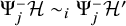



Thus
$\Psi _j^{-}\mathcal {H}\sim \Psi _{j}^{-}\mathcal {H}'$
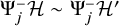 in all cases and the claim is proved. By induction, we get that if
$\mathcal {H}\sim \mathcal {H}'$
in all cases and the claim is proved. By induction, we get that if
$\mathcal {H}\sim \mathcal {H}'$
 in
$\mathrm {QFl}_{n-1}$
in
$\mathrm {QFl}_{n-1}$
 then
$\Psi _j^-\mathcal {H}\sim \Psi _j^-\mathcal {H}'$
then
$\Psi _j^-\mathcal {H}\sim \Psi _j^-\mathcal {H}'$
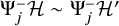 . We apply this to
$\mathcal {G}$
. We apply this to
$\mathcal {G}$
 and
$\operatorname {id}_{\mathrm {Fl}_{n-1}}$
and
$\operatorname {id}_{\mathrm {Fl}_{n-1}}$
 and get
$\Psi _j^-\mathcal {G}\sim \Psi _j^-\operatorname {id}_{\mathrm {Fl}_{n-1}}=\operatorname {id}_{\mathrm {Fl}_{n}}$
and get
$\Psi _j^-\mathcal {G}\sim \Psi _j^-\operatorname {id}_{\mathrm {Fl}_{n-1}}=\operatorname {id}_{\mathrm {Fl}_{n}}$
 , which concludes the proof since
$\mathcal {F}\sim _j\Psi _j^-\mathcal {G}$
, which concludes the proof since
$\mathcal {F}\sim _j\Psi _j^-\mathcal {G}$
 .
.
11 The GKM presentation of
$H^{\bullet }_{T_{n}}(\mathrm {QFl}_{n})$

In this section we give a presentation of
$H^{\bullet }_{T_n}(\mathrm {QFl}_n)$
 and
$H^{\bullet }(\mathrm {QFl}_n)$
and
$H^{\bullet }(\mathrm {QFl}_n)$
 in terms of a certain combinatorially defined “graph cohomology ring,” and describe a free
$\mathbb Z[\textbf {t}_n]$
in terms of a certain combinatorially defined “graph cohomology ring,” and describe a free
$\mathbb Z[\textbf {t}_n]$
 -basis for this ring. These results will be used in the next section to give a Borel-type presentation.
We appeal to GKM theory, which is a technique for computing the equivariant cohomology ring of a variety X under the action of an algebraic torus under suitable hypotheses. While originally developed for rational cohomology by Goresky, Kottwitz, and MacPherson [Reference Goresky, Kottwitz and MacPherson25] with inspiration from Chang and Skjelbred [Reference Chang and Skjelbred17], we present a variant with stricter hypotheses that computes integral cohomology.
Throughout we use the case
$X = \mathrm {Fl}_{n}$
 as a motivating example.
11.1 The GKM ring
Without loss of generality we take
$T = T_{n}$
 . As is standard in algebraic combinatorics, we denote by
$t_{i}$
. As is standard in algebraic combinatorics, we denote by
$t_{i}$
 the negative first Chern class
$-c_{1}^{T}(\mathbb C_{\chi _{i}}) \in H^{2}_{T_{n}}(\operatorname {pt})$
the negative first Chern class
$-c_{1}^{T}(\mathbb C_{\chi _{i}}) \in H^{2}_{T_{n}}(\operatorname {pt})$
 . We then have a homomorphism of abelian groups

The equivariant cohomology ring of a point is freely generated by the
$t_{i}$
 and we identify
$H^{\bullet }_{T_{n}}(\operatorname {pt}) = \mathbb Z[\textbf {t}_{n}]$
and we identify
$H^{\bullet }_{T_{n}}(\operatorname {pt}) = \mathbb Z[\textbf {t}_{n}]$
 , so that all
$T_n$
, so that all
$T_n$
 -equivariant cohomology rings are
$\mathbb Z[\textbf {t}_{n}]$
-equivariant cohomology rings are
$\mathbb Z[\textbf {t}_{n}]$
 -algebras.
For an edge labeled graph G with vertices V, edges E, and edge labels given by a function

we define the
$\color {blue}{{graph\, cohomology\, ring}}$
 for G to be the
$H^{\bullet }_{T_n}(\operatorname {pt})$
for G to be the
$H^{\bullet }_{T_n}(\operatorname {pt})$
 -algebra

with multiplication defined pointwise.
We now describe sufficient conditions for
$H_{T_n}^{\bullet }(G)$
 to be the cohomology ring for a variety X. Say that X has a
$\color {blue}{{good\, affine\, paving}}$
to be the cohomology ring for a variety X. Say that X has a
$\color {blue}{{good\, affine\, paving}}$
 if there is a filtration
$\varnothing =X_0\subset X_1\subset X_2\subset \cdots \subset X_{\ell }=X$
if there is a filtration
$\varnothing =X_0\subset X_1\subset X_2\subset \cdots \subset X_{\ell }=X$
 by closed subvarieties
$X_{i}$
by closed subvarieties
$X_{i}$
 such that for each
$i\ge 1$
such that for each
$i\ge 1$
 the following hold.
-
1. The set $X_i\setminus X_{i-1}$
contains a unique T-fixed point
$p_i$
, and there is a T-equivariant isomorphism of algebraic varieties
$X_i\setminus X_{i-1}\cong V_i$
for some linear T-representation
$V_i$
. -
2. The representation $V_i$
decomposes into a direct sum of one-dimensional T-representations $$\begin{align*}V_i=\bigoplus_{j\in A_i}V_{i,j} \qquad\text{where}\qquad A_i\subset \{1,\ldots,i-1\} \end{align*}$$such that $\overline {V_{i,j}}=V_{i,j}\cup \{p_j\}$
and topologically
$\overline {V_{i,j}}\cong \mathbb {P}^1$
.
-
3. For each $j \in A_{i}$
,
$f_{i,j}=-c_1^T(V_{i, j}) \in H^{\bullet }_{T_n}(G)$
satisfies:-
(a) $f_{i, j} \neq \pm f_{i, k}$
for
$j \neq k$
, and -
(b) $f_{i, j}$
is reduced, meaning that if
$f_{i, j} = a_{1} t_{1} + a_{2} t_{2} + \cdots + a_{n} t_{n}$
, then
$\gcd (a_{1}, a_{2}, \ldots , a_{n}) = 1$
.
-














A good affine paving on X defines a
$\color {blue}{{GKM\, graph}}$
 , which is an undirected, edge-labeled graph
$G_{X}$
, which is an undirected, edge-labeled graph
$G_{X}$
 with vertex set given by the fixed points
$X^{T} = \{p_{1}, \ldots , p_{\ell }\}$
with vertex set given by the fixed points
$X^{T} = \{p_{1}, \ldots , p_{\ell }\}$
 . For each one-dimensional summand
$V_{i, j}$
. For each one-dimensional summand
$V_{i, j}$
 in (2),
$G_{X}$
in (2),
$G_{X}$
 has an edge
$p_{i}p_{j}$
has an edge
$p_{i}p_{j}$
 , and this edge is labeled by
$-c_{1}^T(V_{i, j})$
, and this edge is labeled by
$-c_{1}^T(V_{i, j})$
 .
.
Example 11.1. Let
$X = \mathrm {Fl}_{n}$
 . For any total order
$w_{1}, \ldots , w_{n!}$
. For any total order
$w_{1}, \ldots , w_{n!}$
 of
$S_{n}$
of
$S_{n}$
 that extends the Bruhat order,
$X_{k} = \bigcup _{i = 1}^{k} Bw_{i}B$
that extends the Bruhat order,
$X_{k} = \bigcup _{i = 1}^{k} Bw_{i}B$
 defines a good affine paving. Then
$V_{i} \cong M(w)$
defines a good affine paving. Then
$V_{i} \cong M(w)$
 with
$p_{k} = w_{k}B$
with
$p_{k} = w_{k}B$
 , and following Equation (9.5) we have
$j \in A_{i}$
, and following Equation (9.5) we have
$j \in A_{i}$
 if and only if
$w_{j} = w_{i}(a\,b)$
if and only if
$w_{j} = w_{i}(a\,b)$
 for
$(a, b) \in \operatorname {Inv}(w)$
for
$(a, b) \in \operatorname {Inv}(w)$
 and
$f_{i, j} = t_{w(b)} - t_{w(a)}$
and
$f_{i, j} = t_{w(b)} - t_{w(a)}$
 . It follows that the GKM graph is obtained from
$\operatorname {Cayley}(S_{n})$
. It follows that the GKM graph is obtained from
$\operatorname {Cayley}(S_{n})$
 by labeling edges of the form w to
$(i, j)w$
by labeling edges of the form w to
$(i, j)w$
 by
$t_{j} - t_{i}$
by
$t_{j} - t_{i}$
 .
.
We now consider
$\mathrm {QFl}_{n}$
 . Let
$\operatorname {Cayley}(\operatorname {NC}_{n})$
. Let
$\operatorname {Cayley}(\operatorname {NC}_{n})$
 denote the Hasse diagram of the Kreweras order on
$\operatorname {NC}_{n}$
denote the Hasse diagram of the Kreweras order on
$\operatorname {NC}_{n}$
 as defined in Section 2.2, which is an induced subgraph of
$\operatorname {Cayley}(S_{n})$
as defined in Section 2.2, which is an induced subgraph of
$\operatorname {Cayley}(S_{n})$
 .
.
Theorem 11.2. Theorem 9.7 gives a good affine paving of
$\mathrm {QFl}_{n}$
 , and its GKM graph is obtained from
$\operatorname {Cayley}(\operatorname {NC}_{n})$
, and its GKM graph is obtained from
$\operatorname {Cayley}(\operatorname {NC}_{n})$
 by labeling edges of the form w to
$(i, j)w$
by labeling edges of the form w to
$(i, j)w$
 by
$t_{j} - t_{i}$
by
$t_{j} - t_{i}$
 .
.
Proof. Theorem 9.7 verifies condition (1) directly and shows that
$\mathrm {QFl}_{n}^{T_{n}} = \{wB \;|\; w \in \operatorname {NC}_{n}\}$
 . Conditions (2) and (3) then follow from the fact that our filtration is obtained by intersecting
$\mathrm {QFl}_{n}$
. Conditions (2) and (3) then follow from the fact that our filtration is obtained by intersecting
$\mathrm {QFl}_{n}$
 with a good affine paving for
$\mathrm {Fl}_{n}$
with a good affine paving for
$\mathrm {Fl}_{n}$
 . The same reasoning computes the edges and edge labels for the GKM graph.
Theorem 11.3. If X has a good affine paving, then:
-
1. X has a T-invariant homology basis given by the classes $[\overline {X_i\setminus X_{i-1}}]\in H_\bullet (X)$
, -
2. $H^{\bullet }_T(X)\cong H^{\bullet }_T(G_X)$
, the graph cohomology ring, and -
3. if $H^{\bullet }_T(X)$
is a free
$\mathbb Z[\textbf {t}_n]$
-module, then
$H^{\bullet }_T(X)/\langle t_1,\ldots ,t_n\rangle\cong H^{\bullet }(X)$
.





While variants of Theorem 11.3 appear as [Reference Harada, Henriques and Holm28, Theorem 2.3] and [Reference Goresky, Kottwitz and MacPherson25, Theorem 1.2.2], we did not find the exact statement required for
$\mathrm {QFl}_{n}$
 . Therefore we include a proof for completeness.
Proof. The first part follows from [Reference Fulton21, see Example 1.9.1 and 19.1.11] (in fact the existence of the filtration where each
$X_i\setminus X_{i-1}$
 is isomorphic to an affine space suffices). The second part follows from [Reference Harada, Henriques and Holm28, Theorem 3.1]. The last part follows from the implication
$(iii)\implies (i)$
is isomorphic to an affine space suffices). The second part follows from [Reference Harada, Henriques and Holm28, Theorem 3.1]. The last part follows from the implication
$(iii)\implies (i)$
 of [Reference Franz and Puppe20, Theorem 1.1] after noting that
$(S^1)^n$
of [Reference Franz and Puppe20, Theorem 1.1] after noting that
$(S^1)^n$
 -equivariant cohomology is identical to
$T_n$
-equivariant cohomology is identical to
$T_n$
 -equivariant cohomology because
$\mathbb {C}^\ast \cong \mathbb {R}\times S^1$
-equivariant cohomology because
$\mathbb {C}^\ast \cong \mathbb {R}\times S^1$
 and
$\mathbb {R}$
and
$\mathbb {R}$
 is contractible.
Example 11.4. By Theorem 11.3,
$H^{\bullet }_{T_{n}}(\mathrm {Fl}_{n})$
 is isomorphic to the graph cohomology ring

Moreover, the
$[X^{w}] = [\overline {BwB}]$
 give a homology basis for
$H_{\bullet }(\mathrm {Fl}_{n})$
give a homology basis for
$H_{\bullet }(\mathrm {Fl}_{n})$
 .
.
From Theorem 11.2, we obtain the following corollary about
$\mathrm {QFl}_{n}$
 .
.
Corollary 11.5. We have

Further recall that the affine charts from Proposition 9.13 have closures
$X(F)$
 for
$F \in \operatorname {\mathsf {Forest}}_{n}$
for
$F \in \operatorname {\mathsf {Forest}}_{n}$
 .
.
Corollary 11.6. The homology group
$H_{\bullet }(\mathrm {QFl}_{n})$
 has a homology basis
$[X(F)]$
has a homology basis
$[X(F)]$
 for
$F \in \operatorname {\mathsf {Forest}}_{n}$
for
$F \in \operatorname {\mathsf {Forest}}_{n}$
 .
.
Remark 11.7. Simple generalizations of Theorem 11.3 exist to compute generalized cohomology theories such as equivariant K-theory. However, determining a good basis for the resulting rings is a combinatorially specific task which does not transfer easily between theories.
11.2 Flowup bases and double forest polynomials
The following definition characterizes a distinguished subset of
$H_{T_n}^{\bullet }(G)$
 ; the reader should compare this to the definition of generating family by Guillemin–Zara [Reference Guillemin and Zara27, Definition 2.3] or that of canonical classes by Tymoczko [Reference Tymoczko45, §2.2].
Definition 11.8. Let
$G=(V,E,\chi )$
 be a GKM graph. Given a partial ordering
$\le $
be a GKM graph. Given a partial ordering
$\le $
 on V, a
$\color {blue}{{flowup\, basis}}$
on V, a
$\color {blue}{{flowup\, basis}}$
 for
$H_{T_n}^{\bullet }(G)$
for
$H_{T_n}^{\bullet }(G)$
 is a collection of elements
$\{f_v\;|\; v\in V\}\subset H^{\bullet }_{T_n}(G)$
is a collection of elements
$\{f_v\;|\; v\in V\}\subset H^{\bullet }_{T_n}(G)$
 such that
-
(1) $(f_v)_w=0$
if
$v\not \le w$
, and -
(2) $(f_v)_v=\pm \prod _{uv\in E\text { and }u\le v} \chi (uv)$
.



The following fact is classical and a key tool for producing
$\mathbb Z[\textbf {t}_n]$
 -bases for
$H^{\bullet }_{T_n}(G)$
-bases for
$H^{\bullet }_{T_n}(G)$
 .
.
Proposition 11.9. Any flowup basis is a free
$\mathbb Z[\textbf {t}_n]$
 -basis for
$H^{\bullet }_{T_n}(G)$
-basis for
$H^{\bullet }_{T_n}(G)$
 .
.
Proof. An outline of the classical proof can be found in [Reference Tymoczko45, §2.2].
In this section we describe a flowup basis for
$H^{\bullet }_{T_{n}}(\mathrm {QFl}_{n})$
 using the double forest polynomials defined in [Reference Bergeron, Gagnon, Nadeau, Spink and Tewari6]. For
$w \in S_{n}$
using the double forest polynomials defined in [Reference Bergeron, Gagnon, Nadeau, Spink and Tewari6]. For
$w \in S_{n}$
 , let
, let

Example 11.10. Consider the graph cohomology ring for
$\mathrm {Fl}_{n}$
 from Example 11.4. Taking
$\le $
from Example 11.4. Taking
$\le $
 to be the Bruhat order on
$S_{n}$
to be the Bruhat order on
$S_{n}$
 , we have a flowup basis with

where
$\mathfrak {S}_{v}(\textbf {x}_{n}; \textbf {t}_{n})$
 is the double Schubert polynomial; see Section 12.1. The fact that conditions (1) and (2) in Definition 11.8 are met is nontrivial but follows from the AJS–Billey theorem [Reference Andersen, Jantzen and Soergel2, Reference Billey12].
The analogous statement for
$\mathrm {QFl}_{n}$
 makes use of the double forest polynomials defined in [Reference Bergeron, Gagnon, Nadeau, Spink and Tewari6, §4], which we denote by
$\mathfrak {P}_{F}(\textbf {x}_{n}, \textbf {t}_{n}) \in \mathbb Z[\textbf {x}_{n}][\textbf {t}_{n}]$
makes use of the double forest polynomials defined in [Reference Bergeron, Gagnon, Nadeau, Spink and Tewari6, §4], which we denote by
$\mathfrak {P}_{F}(\textbf {x}_{n}, \textbf {t}_{n}) \in \mathbb Z[\textbf {x}_{n}][\textbf {t}_{n}]$
 for each
$F \in \operatorname {\mathsf {Forest}}_{n}$
for each
$F \in \operatorname {\mathsf {Forest}}_{n}$
 . As with Schubert polynomials, we postpone a precise definition of double forest polynomials to Section 12.2.
Theorem 11.11. Taking
$\le $
 to be the Bruhat order restricted to
$\operatorname {NC}_{n}$
to be the Bruhat order restricted to
$\operatorname {NC}_{n}$
 , double forest polynomials define a flowup basis for the graph cohomology ring
$H^{\bullet }_{T_{n}}(\operatorname {Cayley}(\operatorname {NC}_{n}))$
, double forest polynomials define a flowup basis for the graph cohomology ring
$H^{\bullet }_{T_{n}}(\operatorname {Cayley}(\operatorname {NC}_{n}))$
 . Specifically, for
$v,w\in \operatorname {NC}_n$
. Specifically, for
$v,w\in \operatorname {NC}_n$
 we have

where
$F\in \operatorname {\mathsf {Forest}}_n$
 is the unique forest such that
$v=\operatorname {ForToNC}(F)$
is the unique forest such that
$v=\operatorname {ForToNC}(F)$
 .
.
Proof. The claim follows from the analogue of the AJS–Billey theorem for double forest polynomials proved in [Reference Bergeron, Gagnon, Nadeau, Spink and Tewari6, §8]. In particular, [Reference Bergeron, Gagnon, Nadeau, Spink and Tewari6, Theorem 8.14] shows that
$(f_{v})_{w} = 0$
 whenever
$v \not \le w$
whenever
$v \not \le w$
 , and [Reference Bergeron, Gagnon, Nadeau, Spink and Tewari6, Theorem 8.17] shows that
$(f_{v})_{v} = \prod _{(i, j) \in \operatorname {Inv}_{\operatorname {NC}}(v)}( t_{v(j)} - t_{v(i)})$
, and [Reference Bergeron, Gagnon, Nadeau, Spink and Tewari6, Theorem 8.17] shows that
$(f_{v})_{v} = \prod _{(i, j) \in \operatorname {Inv}_{\operatorname {NC}}(v)}( t_{v(j)} - t_{v(i)})$
 .
.
Figure 14 shows one element of the flowup basis for
$H^{\bullet }_{T_{n}}(\operatorname {Cayley}(\operatorname {NC}_{n}))$
 .
.
The flowup basis element of
$H^{\bullet }_{T_{4}}(\operatorname {Cayley}(\operatorname {NC}_{4}))$
 indexed by
$(4\, 3\, 1)$
indexed by
$(4\, 3\, 1)$
 . This is an evaluation of the double forest polynomial for
$F = \widehat {F}(\mathsf {r}_{1}^{-}\mathsf {e}_{1}\mathsf {e}_{1}\mathsf {e}_{2})$
. This is an evaluation of the double forest polynomial for
$F = \widehat {F}(\mathsf {r}_{1}^{-}\mathsf {e}_{1}\mathsf {e}_{1}\mathsf {e}_{2})$
 . For clarity we have set
$\alpha _{ij}:= t_j-t_i$
. For clarity we have set
$\alpha _{ij}:= t_j-t_i$
 .
.
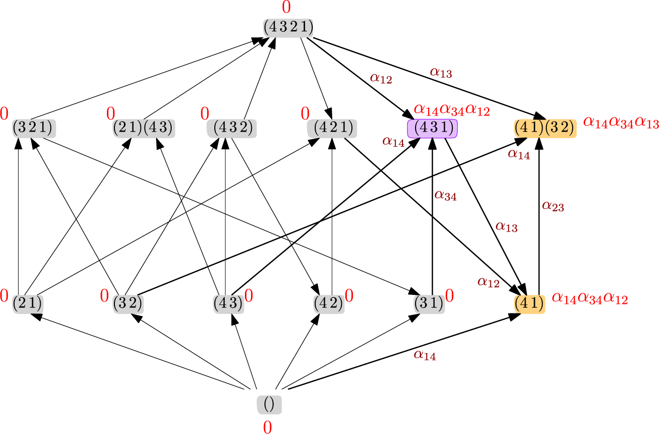
Figure 14 Long description
The diagram consists of nodes arranged in four horizontal levels connected by directed arrows.
* Level 1 (Bottom): A single grey node labeled ( ) with a red 0 below it. Six arrows point upward to Level 2.
* Level 2: Six nodes from left to right. Grey nodes (2 1), (3 2), (4 3), (4 2), and (3 1) all have a red 0 to their left or right. The rightmost node (4 1) is highlighted in orange with a red label alpha sub 1 4 alpha sub 3 4 alpha sub 1 2. An arrow labeled alpha sub 1 4 points from ( ) to (4 1).
* Level 3: Six nodes. From left to right, grey nodes (3 2 1), (2 1)(4 3), (4 3 2), and (4 2 1) all have red 0 labels. The fifth node (4 3 1) is highlighted in purple with a red label alpha sub 1 4 alpha sub 3 4 alpha sub 1 2. The sixth node (4 1)(3 2) is highlighted in orange with a red label alpha sub 1 4 alpha sub 3 4 alpha sub 1 3.
* Level 4 (Top): A single grey node labeled (4 3 2 1) with a red 0 above it.
Key edge labels include alpha sub 1 2 and alpha sub 1 3 pointing from the top node down to the orange and purple nodes. Other internal edges are labeled with alpha sub 1 4, alpha sub 3 4, alpha sub 1 2, alpha sub 1 3, and alpha sub 2 3, indicating the flow of polynomial evaluations between the indexed basis elements.
12 The Borel presentation of
$H^{\bullet }_{T_{n}}(\mathrm {QFl}_{n})$

12.1 Recollections on the equivariant cohomology of
$\mathrm {Fl}_{m}$

We begin by briefly reviewing key aspects of the equivariant cohomology of the complete flag variety that are relevant to us. The reader is referred to [Reference Anderson and Fulton3] for a more complete exposition.
The following is due to Borel [Reference Borel15]. The equivariant cohomology ring
$H^{\bullet }_{T_{m}}(\mathrm {Fl}_{m})$
 is generated by the character lattice of
$T_{m}$
is generated by the character lattice of
$T_{m}$
 and the Chern classes
$c_1^{T_{m}}(\mathcal {F}_i/\mathcal {F}_{i-1})\in H^{2}_{T_{m}}(\mathrm {Fl}_{m})$
and the Chern classes
$c_1^{T_{m}}(\mathcal {F}_i/\mathcal {F}_{i-1})\in H^{2}_{T_{m}}(\mathrm {Fl}_{m})$
 . We therefore have a map
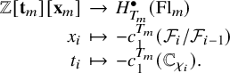
The kernel of this map is the ideal
$\operatorname {ESym}_{m}^+ = \langle f(x_1,\ldots ,x_m)-f(t_1,\ldots ,t_m):f\in \operatorname {Sym}_{m}\rangle$
 , where
$\operatorname {Sym}_{m}$
, where
$\operatorname {Sym}_{m}$
 denotes the ring of symmetric polynomials in
$\textbf {x}_{m}$
denotes the ring of symmetric polynomials in
$\textbf {x}_{m}$
 . Thus, going forward, we identify

In light of the GKM presentation of
$H^{\bullet }_{T_{m}}(\mathrm {Fl}_{m})$
 given in Example 11.4, Borel’s presentation has the following meaning. The inclusion of each torus fixed point
$wB \in \mathrm {Fl}_{m}$
given in Example 11.4, Borel’s presentation has the following meaning. The inclusion of each torus fixed point
$wB \in \mathrm {Fl}_{m}$
 gives a pullback map

In Borel’s presentation, we have
$\operatorname {ev}_{w}(x_{i}) = t_{w(i)}$
 and
$\operatorname {ev}_{w}(t_{i}) = t_{i}$
and
$\operatorname {ev}_{w}(t_{i}) = t_{i}$
 , so we can identify
$\operatorname {ev}_{w}$
, so we can identify
$\operatorname {ev}_{w}$
 with the map of the same name defined on polynomials in (11.1). In other words, the map

surjects onto the graph cohomology ring
$H^{\bullet }_{T_{m}}(\operatorname {Cayley}(S_{m})) \subseteq \mathbb Z[\textbf {t}_{m}]^{\oplus S_{m}}$
 .
.
Now let X be an algebraic variety with an action of
$T_{m}$
 and
$Z \subseteq X$
and
$Z \subseteq X$
 a
$T_{m}$
a
$T_{m}$
 -invariant subvariety. For a cohomology class
$f \in H^{\bullet }_{T_{m}}(X)$
-invariant subvariety. For a cohomology class
$f \in H^{\bullet }_{T_{m}}(X)$
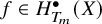 , we denote the
$T_{m}$
, we denote the
$T_{m}$
 -equivariant degree of f on Z by

where
$\kappa ^Z$
 denotes the unique map
$Z \to \operatorname {pt}$
denotes the unique map
$Z \to \operatorname {pt}$
 ,
$\mathbb {1}_{Z} \in H^{\bullet }_{T_{m}}(X)$
,
$\mathbb {1}_{Z} \in H^{\bullet }_{T_{m}}(X)$
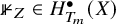 is the pushforward of
$1\in {H^{\bullet }_{T_{m}}(Z)}$
is the pushforward of
$1\in {H^{\bullet }_{T_{m}}(Z)}$
 along the inclusion
$\iota : Z \to X$
along the inclusion
$\iota : Z \to X$
 , and the equality
$\kappa ^Z_*(\iota ^*f)=\kappa ^X_{\ast } (\mathbb {1}_{Z} f)$
, and the equality
$\kappa ^Z_*(\iota ^*f)=\kappa ^X_{\ast } (\mathbb {1}_{Z} f)$
 is the push–pull formula.
Borel’s presentation provides a simple way to compute the degree on a Schubert variety using the
$\color {blue}{{divided\, difference\, operations}}\, \partial _{i}: \mathbb Z[\textbf {t}_{m}][\textbf {x}_{m}] \to \mathbb Z[\textbf {t}_{m}][\textbf {x}_{m}]$
 defined by

Recall the forgetful map
$\pi _{i} \colon \mathrm {Fl}_{n}\to \mathrm {GL}_{m}/P_i$
 from Section 3.2. The following is due to Bernstein–Gelfand–Gelfand [Reference Bernšteĭn, Gelfand and Gelfand8] and Demazure [Reference Demazure19]; see [Reference Anderson and Fulton3, Chapter 10, Lemma 6.5] for textbook treatment.
Proposition 12.1. The map
$(\pi _i)^*(\pi _i)_*:H^{\bullet }_{T_{m}}(\mathrm {Fl}_{m})\to H^{\bullet }_{T_{m}}(\mathrm {Fl}_{m})$
 is given by
$f\mapsto \partial _i f$
is given by
$f\mapsto \partial _i f$
 . Moreover, for
$w \in S_{m}$
. Moreover, for
$w \in S_{m}$
 with
$w(i) < w(i+1)$
with
$w(i) < w(i+1)$
 , we have
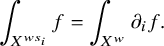
The
$\color {blue}{{double\, Schubert\, polynomials}}$
 are the unique family of polynomials
$\{\mathfrak {S}_{w}(\textbf {x}_{m}; \textbf {t}_{m}) \;|\; w \in S_{m}\}$
are the unique family of polynomials
$\{\mathfrak {S}_{w}(\textbf {x}_{m}; \textbf {t}_{m}) \;|\; w \in S_{m}\}$
 such that each
$\mathfrak {S}_{w}(\textbf {x}_{m}; \textbf {t}_{m})$
such that each
$\mathfrak {S}_{w}(\textbf {x}_{m}; \textbf {t}_{m})$
 does not depend on
$x_{m}$
does not depend on
$x_{m}$
 and moreover satisfies

We therefore have a
$T_{m}$
 -equivariant Kronecker duality between double Schubert polynomials and the homology basis of Schubert cycles
$[X^{w}]$
-equivariant Kronecker duality between double Schubert polynomials and the homology basis of Schubert cycles
$[X^{w}]$
 described in Example 11.4, as we have
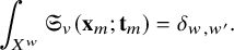
In the following subsections, we tell a parallel story for
$\mathrm {QFl}_{m}$
 using equivariantly quasisymmetric polynomials and double forest polynomials.
Remark 12.2. Borel’s presentation for ordinary cohomology is
$H^{\bullet }(\mathrm {Fl}_{m}) \cong \mathbb Z[\textbf {x}_{m}]/\operatorname {Sym}_{m}^+$
 , which can be recovered from the equivariant version by setting
$t_{i} \mapsto 0$
, which can be recovered from the equivariant version by setting
$t_{i} \mapsto 0$
 , as is formalized in Theorem 11.3.
12.2 Borel’s theorem for equivariant quasisymmetry
In order to state our analogue of Borel’s theorem, we review several aspects of equivariant quasisymmetry from [Reference Bergeron, Gagnon, Nadeau, Spink and Tewari6]. In Section 12.3, we will give geometric interpretations which motivate these definitions. We define the
$\color {blue}{{equivariant\, Bergeron{-}Sottile\, maps}}$


and the
$\color {blue}{{equivariant\, quasisymmetric\, divided\, difference}}$


The
$\color {blue}{{double\, forest\, polynomials}}$
 are then the unique family of polynomials
$\{\mathfrak {P}_{F}(\textbf {x}_n;\textbf {t}_n)\;|\; F\in \operatorname {\mathsf {Forest}}_{n} \}$
are then the unique family of polynomials
$\{\mathfrak {P}_{F}(\textbf {x}_n;\textbf {t}_n)\;|\; F\in \operatorname {\mathsf {Forest}}_{n} \}$
 such that each
$\mathfrak {P}_{F}(\textbf {x}_{n};\textbf {t}_{n})$
such that each
$\mathfrak {P}_{F}(\textbf {x}_{n};\textbf {t}_{n})$
 does not depend on
$x_{n}$
does not depend on
$x_{n}$
 and moreover satisfies

where
$\textbf {t}_{[n]/\{i\}} = (t_{1}, \ldots , t_{i-1}, t_{i+1}, \ldots , t_{n})$
 .
.
Remark 12.3. While it is not immediately obvious from the definition, [Reference Bergeron, Gagnon, Nadeau, Spink and Tewari6, Corollary 4.8] shows that double forest polynomials have the following stability property: for each
$F \in \operatorname {\mathsf {Forest}}_{n-1}$
 , we have
$\mathfrak {P}_{F}(\textbf {x}_{n-1}; \textbf {t}_{n-1}) = \mathfrak {P}_{F \cdot \mathsf {r}_{n}^{-}}(\textbf {x}_{n}; \textbf {t}_{n})$
, we have
$\mathfrak {P}_{F}(\textbf {x}_{n-1}; \textbf {t}_{n-1}) = \mathfrak {P}_{F \cdot \mathsf {r}_{n}^{-}}(\textbf {x}_{n}; \textbf {t}_{n})$
 as polynomials.
The ring of
$\color {blue}{{equivariantly\, quasisymmetric\, polynomials}}\, \text{EQSym}_{n}$
 is
is

which is a subring of
$\mathbb Z[\textbf {t}_{n}][\textbf {x}_{n}]$
 . We also denote
$\text{EQSym}_{n}^+ = \langle f(\textbf {x}_{n}; \textbf {t}_{n}) - f(\textbf {t}_{n}; \textbf {t}_{n}) \;|\; f \in \text{EQSym}_{n} \rangle$
. We also denote
$\text{EQSym}_{n}^+ = \langle f(\textbf {x}_{n}; \textbf {t}_{n}) - f(\textbf {t}_{n}; \textbf {t}_{n}) \;|\; f \in \text{EQSym}_{n} \rangle$
 .
.
Theorem 12.4. We have

and moreover the double forest polynomials
$\mathfrak {P}_{F}(\textbf {x}_{n}; \textbf {t}_{n})$
 where
$F\in \operatorname {\mathsf {Forest}}_n$
where
$F\in \operatorname {\mathsf {Forest}}_n$
 give a free
$\mathbb Z[\textbf {t}_{n}]$
give a free
$\mathbb Z[\textbf {t}_{n}]$
 -basis for this ring.
Our proof primarily relies on results from Section 11, but we make use of one result which is deferred to Appendix A for ease of exposition.
Proof. By Theorem 11.3, we know that
$H^{\bullet }_{T_{n}}(\mathrm {QFl}_{n})$
 is isomorphic to the graph cohomology ring
$H^{\bullet }_{T_{n}}(\operatorname {Cayley}(\operatorname {NC}_{n})) \subseteq \mathbb Z[\textbf {t}_{n}]^{\operatorname {NC}_{n}}$
is isomorphic to the graph cohomology ring
$H^{\bullet }_{T_{n}}(\operatorname {Cayley}(\operatorname {NC}_{n})) \subseteq \mathbb Z[\textbf {t}_{n}]^{\operatorname {NC}_{n}}$
 . We prove the theorem by showing that the map

induces the desired isomorphism onto the graph cohomology ring.
The image of
$\mathbf {ev}_{\operatorname {NC}}$
 is contained in the graph cohomology ring, as for any permutation w,
$t_{b} - t_{a}$
is contained in the graph cohomology ring, as for any permutation w,
$t_{b} - t_{a}$
 divides
$\operatorname {ev}_{w}(f) - \operatorname {ev}_{(a\,b)w}(f)$
divides
$\operatorname {ev}_{w}(f) - \operatorname {ev}_{(a\,b)w}(f)$
 . Moreover, by Theorem 11.11, the double forest polynomials map to a free (flowup) basis of
$H^{\bullet }_{T_{n}}(\operatorname {Cayley}(\operatorname {NC}_{n}))$
. Moreover, by Theorem 11.11, the double forest polynomials map to a free (flowup) basis of
$H^{\bullet }_{T_{n}}(\operatorname {Cayley}(\operatorname {NC}_{n}))$
 , so
$\mathbf {ev}_{\operatorname {NC}}$
, so
$\mathbf {ev}_{\operatorname {NC}}$
 is surjective.
What remains is to show that
$\ker (\mathbf {ev}_{\operatorname {NC}}) = \text{EQSym}_{n}^+$
 , which is Theorem A.1 in Appendix A.
We finally consider ordinary cohomology, proving Theorem A. As in the introduction, write
$\text{QSym}_{n}^+$
 for the ideal generated by quasisymmetric polynomials with no constant term.
Corollary 12.5. We have

Moreover, the forest polynomials
$\mathfrak {P}_{F}(\textbf {x}_{n}; 0)$
 where
$F\in \operatorname {\mathsf {Forest}}_n$
where
$F\in \operatorname {\mathsf {Forest}}_n$
 give a free
$\mathbb Z$
give a free
$\mathbb Z$
 -basis for this ring.
Proof. By Theorem 11.3, we can obtain
$H^{\bullet }(\mathrm {QFl}_{n})$
 from
$H^{\bullet }_{T_{n}}(\mathrm {QFl}_{n})$
from
$H^{\bullet }_{T_{n}}(\mathrm {QFl}_{n})$
 by performing a change of scalars along the homomorphism
$\mathbb Z[\textbf {t}_{n}] \to \mathbb Z$
by performing a change of scalars along the homomorphism
$\mathbb Z[\textbf {t}_{n}] \to \mathbb Z$
 given by
$t_{i} \mapsto 0$
given by
$t_{i} \mapsto 0$
 . Applying this base change to our Borel presentation, we have a canonical identification between the images of
$\mathbb Z[\textbf {t}_{n}][\textbf {x}_{n}]$
. Applying this base change to our Borel presentation, we have a canonical identification between the images of
$\mathbb Z[\textbf {t}_{n}][\textbf {x}_{n}]$
 ,
$\text{EQSym}_{n}$
,
$\text{EQSym}_{n}$
 ,
$\text{EQSym}_{n}^+$
,
$\text{EQSym}_{n}^+$
 , and
$\mathfrak {P}_{F}(\textbf {x}_{n}; \textbf {t}_{n})$
, and
$\mathfrak {P}_{F}(\textbf {x}_{n}; \textbf {t}_{n})$
 with
$\mathbb Z[\textbf {x}_{n}]$
with
$\mathbb Z[\textbf {x}_{n}]$
 ,
$\text{QSym}_{n}$
,
$\text{QSym}_{n}$
 ,
$\text{QSym}_{n}^+$
,
$\text{QSym}_{n}^+$
 , and
$\mathfrak {P}_{F}(\textbf {x}_{n}; 0)$
, and
$\mathfrak {P}_{F}(\textbf {x}_{n}; 0)$
 .
.
12.3 Geometric realizations of
$\mathsf {R}_{i}^{\pm }$
and
${\mathsf {E}_{i}}$


We now show that the equivariant Bergeron–Sottile maps correspond to equivariant cohomology operations that are adjoint to the building maps
$\Psi _{i,j}$
 and
$\mathbb {P}_i$
and
$\mathbb {P}_i$
 defined in Section 3.
Fact 12.6. Let
$\gamma :T\to T'$
 be a coordinate projection between two algebraic tori T and
$T'$
be a coordinate projection between two algebraic tori T and
$T'$
 . For X a variety with a T-action, we have

Furthermore, if
$\Phi :X\to Y$
 is a
$T'$
is a
$T'$
 -equivariant map of varieties with a
$T'$
-equivariant map of varieties with a
$T'$
 -action, then
$\Phi ^*:H^{\bullet }_{T}(Y)\to H^{\bullet }_{T}(X)$
-action, then
$\Phi ^*:H^{\bullet }_{T}(Y)\to H^{\bullet }_{T}(X)$
 and
$\Phi _*:H^{\bullet }_{T}(X)\to H^{\bullet }_{T}(Y)$
and
$\Phi _*:H^{\bullet }_{T}(X)\to H^{\bullet }_{T}(Y)$
 are given by extending the corresponding maps on
$T'$
are given by extending the corresponding maps on
$T'$
 -equivariant cohomology by the identity map on
$H^{\bullet }_{T}(\operatorname {pt})$
-equivariant cohomology by the identity map on
$H^{\bullet }_{T}(\operatorname {pt})$
 .
.
As in Definition 3.2, we write
$\gamma _{i}: T_{m} \to T_{m-1}$
 for the i-th coordinate projection and
$\mathrm {Fl}_{m-1}^{\gamma _i}$
for the i-th coordinate projection and
$\mathrm {Fl}_{m-1}^{\gamma _i}$
 for
$\mathrm {Fl}_{m-1}$
for
$\mathrm {Fl}_{m-1}$
 with the action of
$T_{m}$
with the action of
$T_{m}$
 induced by
$\gamma _{i}$
induced by
$\gamma _{i}$
 . With Fact 12.6, the GKM presentation of the
$T_{m-1}$
. With Fact 12.6, the GKM presentation of the
$T_{m-1}$
 -equivariant cohomology of
$\mathrm {Fl}_{m-1}$
-equivariant cohomology of
$\mathrm {Fl}_{m-1}$
 implies that

and the Borel presentation similarly implies

The isomorphism between these two presentations is given by

Proposition 12.7. The pullback map
$\Psi _{i,j}^*\colon H^{\bullet }_{T_m}(\mathrm {Fl}_{m})\to H^{\bullet }_{T_m}(\mathrm {Fl}_{m-1}^{\gamma _i})$
 sends
$t_k\mapsto t_k$
sends
$t_k\mapsto t_k$
 for all k, and
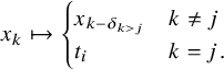
Proof. We have that
$\Psi _{i,j}^*t_k=t_k$
 holds since
$\Psi _{i,j}$
holds since
$\Psi _{i,j}$
 is a
$T_m$
is a
$T_m$
 -equivariant map, so it suffices to show the result for
$x_k$
-equivariant map, so it suffices to show the result for
$x_k$
 . To avoid notational overlap, we will let
$x_1^{\gamma _i},\ldots ,x_{m-1}^{\gamma _i}$
. To avoid notational overlap, we will let
$x_1^{\gamma _i},\ldots ,x_{m-1}^{\gamma _i}$
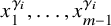 denote the
$x_i$
denote the
$x_i$
 generators in
$\mathrm {Fl}_{m-1}^{\gamma _i}$
generators in
$\mathrm {Fl}_{m-1}^{\gamma _i}$
 . It suffices to show that for all
$w \in S_{m-1}$
. It suffices to show that for all
$w \in S_{m-1}$


Note that
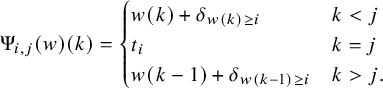
For
$w\in S_{m-1}$
 we have
$\operatorname {ev}_{w}(x_\ell ^{\gamma _i}) =\gamma _i^* t_{w(\ell )}=t_{w(\ell )+\delta _{w(\ell )\ge i}}$
we have
$\operatorname {ev}_{w}(x_\ell ^{\gamma _i}) =\gamma _i^* t_{w(\ell )}=t_{w(\ell )+\delta _{w(\ell )\ge i}}$
 , and therefore for
$k\ne j$
, and therefore for
$k\ne j$
 we have

On the other hand, because
$\operatorname {ev}_w$
 and
$\operatorname {ev}_{\Psi _{i,j}(w)}$
and
$\operatorname {ev}_{\Psi _{i,j}(w)}$
 are pullbacks under the inclusions
$\{w\}\hookrightarrow \mathrm {Fl}_{m-1}^{\gamma _i}$
are pullbacks under the inclusions
$\{w\}\hookrightarrow \mathrm {Fl}_{m-1}^{\gamma _i}$
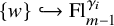 and
$\{\Psi _{i,j}(w)\}\hookrightarrow \mathrm {Fl}_{m}$
and
$\{\Psi _{i,j}(w)\}\hookrightarrow \mathrm {Fl}_{m}$
 , we have

Proposition 12.8. The maps
$(\Psi _i^{\pm })^*:H^{\bullet }_{T_m}(\mathrm {Fl}_{m})\to H^{\bullet }_{T_m}(\mathrm {Fl}_{m-1}^{\gamma _i})$
 are given by

The map
$(\Psi _i^{\pm })^*(\pi _i)^*(\pi _i)_*:H^{\bullet }_{T_m}(\mathrm {Fl}_{m})\to H^{\bullet }_{T_m}(\mathrm {Fl}_{m-1}^{\gamma _i})$
 is given by

Proof. Specializing the computation of
$\Psi _{i,j}^*$
 in Proposition 12.7 to
$j=i,i+1$
in Proposition 12.7 to
$j=i,i+1$
 gives (12.2). Since
$(\pi _i)^*(\pi _i)_*$
gives (12.2). Since
$(\pi _i)^*(\pi _i)_*$
 computes
$\partial _i$
computes
$\partial _i$
 by Proposition 12.1, we obtain (12.3) from the identity
${\mathsf {E}_{i}}f=\mathsf {R}_{i}^{\pm }\partial _if$
by Proposition 12.1, we obtain (12.3) from the identity
${\mathsf {E}_{i}}f=\mathsf {R}_{i}^{\pm }\partial _if$
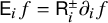 .
.
Theorem 12.9. Let
$Z\subset \mathrm {Fl}_{m-1}^{\gamma _i}$
 be a
$T_{m}$
be a
$T_{m}$
 -invariant subvariety. Then for
$f\in H^{\bullet }_{T_m}(\mathrm {Fl}_{m})$
-invariant subvariety. Then for
$f\in H^{\bullet }_{T_m}(\mathrm {Fl}_{m})$
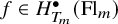 , we have equalities of
$T_{m}$
, we have equalities of
$T_{m}$
 -equivariant degrees

Proof. As the
$\Psi _i^{\pm }$
 are closed embeddings we have
$\mathbb {1}_{\Psi _i^{\pm }Z} = (\Psi _{i}^{\pm })_* \mathbb {1}_{Z}\in H^{\bullet }_{T_m}(\mathrm {Fl}_{m})$
are closed embeddings we have
$\mathbb {1}_{\Psi _i^{\pm }Z} = (\Psi _{i}^{\pm })_* \mathbb {1}_{Z}\in H^{\bullet }_{T_m}(\mathrm {Fl}_{m})$
 . The first degree equation now comes from

where we used the push-pull formula in all three equalities. For the second degree equation, because the
$\pi _i\Psi _i$
 are closed embeddings, we have

Therefore using a similar argument as above,

where the last equality uses (12.3). This establishes the second part of (12.4).
12.4 The degree on
$X(\widehat {F})$
using the
$\star $
-monoid


We now describe a combinatorial procedure for computing the degree on the
$X(\widehat {F})$
 varieties using the
$\color {blue}{\star{-}\textit{monoid}\, \mathcal {S}}$
varieties using the
$\color {blue}{\star{-}\textit{monoid}\, \mathcal {S}}$
 from [Reference Bergeron, Gagnon, Nadeau, Spink and Tewari6, §9.2]. For each
$A \subseteq [n]$
from [Reference Bergeron, Gagnon, Nadeau, Spink and Tewari6, §9.2]. For each
$A \subseteq [n]$
 , writing
$A=(i_1<\cdots < i_k)$
, writing
$A=(i_1<\cdots < i_k)$
 , we define a map

the coordinate projection away from
$i_1,\ldots ,i_k$
 . To compose these maps, we define an operation on subsets
$A,B\subset [n]$
. To compose these maps, we define an operation on subsets
$A,B\subset [n]$
 with
$|A| + |B| \le n$
with
$|A| + |B| \le n$
 :
:

where
$([n] \setminus B)_i$
 denotes the i-th element of
$[n] \setminus B$
denotes the i-th element of
$[n] \setminus B$
 in increasing order. The following proposition is straightforward and we omit the proof.
Proposition 12.10. For
$A, B \subseteq [n]$
 with
$|A| + |B| \le n$
with
$|A| + |B| \le n$
 ,
$\gamma _{A} \circ \gamma _{B} = \gamma _{A\star B}$
,
$\gamma _{A} \circ \gamma _{B} = \gamma _{A\star B}$
 . In particular,
$\gamma _i \circ \gamma _A =\gamma _{i \star A}$
. In particular,
$\gamma _i \circ \gamma _A =\gamma _{i \star A}$
 .
.
We let
$\mathrm {Fl}_{[n]/A}$
 denote
$\mathrm {Fl}_{n-|A|}^{\gamma _A}$
denote
$\mathrm {Fl}_{n-|A|}^{\gamma _A}$
 , and let
$X(\widehat {G})_{[n]/A}$
, and let
$X(\widehat {G})_{[n]/A}$
 denote
$X(\widehat {G})\subset \mathrm {Fl}_{n-|A|}^{\gamma _A}$
denote
$X(\widehat {G})\subset \mathrm {Fl}_{n-|A|}^{\gamma _A}$
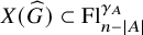 equipped with the torus action of
$T_{n}$
equipped with the torus action of
$T_{n}$
 induced by
$\gamma _A$
induced by
$\gamma _A$
 . Taken in conjunction with Fact 12.6, this allows us to transfer our results about the
$T_m$
. Taken in conjunction with Fact 12.6, this allows us to transfer our results about the
$T_m$
 -varieties
$\mathrm {Fl}_{m}$
-varieties
$\mathrm {Fl}_{m}$
 and
$\mathrm {Fl}_{m-1}^{\gamma _i}$
and
$\mathrm {Fl}_{m-1}^{\gamma _i}$
 to results about the
$T_n$
to results about the
$T_n$
 -varieties
$\mathrm {Fl}_{[n]/A}$
-varieties
$\mathrm {Fl}_{[n]/A}$
 and
$\mathrm {Fl}_{[n]/(i\star A)}$
and
$\mathrm {Fl}_{[n]/(i\star A)}$
 .
.
For
$A \subseteq [n]$
 , we denote
$t_{i, A} = t_{([n] \setminus A)_{i}}$
, we denote
$t_{i, A} = t_{([n] \setminus A)_{i}}$
 and
$\textbf {t}_{[n]/A} = (t_{1, A}, t_{2, A}, \ldots , t_{n-|A|, A})$
and
$\textbf {t}_{[n]/A} = (t_{1, A}, t_{2, A}, \ldots , t_{n-|A|, A})$
 . We have isomorphisms

and a GKM presentation

with the isomorphism between the Borel presentation and the GKM presentation given by

For
$f\in \mathbb Z[\textbf {t}_n][\textbf {x}_n]$
 define
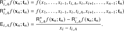
Definition 12.11. For
$A \subseteq [n]$
 and
$\Omega \in \mathrm {RESeq}_{n - |A|}$
and
$\Omega \in \mathrm {RESeq}_{n - |A|}$
 , let
, let
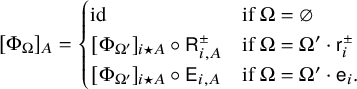
For
$\Omega \in \mathrm {RESeq}_{n}$
 we write
$[\Phi _{\Omega }] = [\Phi _{\Omega }]_{\varnothing }$
we write
$[\Phi _{\Omega }] = [\Phi _{\Omega }]_{\varnothing }$
 .
.
As was shown in [Reference Bergeron, Gagnon, Nadeau, Spink and Tewari6, Theorem 10.5], the operation
$[\Phi _{\Omega }]$
 only depends on the colored Tamari equivalence class of the bicolored nested forest
$\widehat {F}(\Omega )$
only depends on the colored Tamari equivalence class of the bicolored nested forest
$\widehat {F}(\Omega )$
 associated to
$\Omega $
associated to
$\Omega $
 ; we can write
$[\Phi _{\widehat {F}}]$
; we can write
$[\Phi _{\widehat {F}}]$
 for
$\widehat {F} \in \operatorname {BNestFor}_{n}$
for
$\widehat {F} \in \operatorname {BNestFor}_{n}$
 without ambiguity.
Theorem 12.12. For
$\widehat {F}\in \operatorname {BNestFor}_n$
 and
$f \in H^{\bullet }_{T_{n}}(\mathrm {Fl}_{n})$
and
$f \in H^{\bullet }_{T_{n}}(\mathrm {Fl}_{n})$
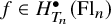 , we have
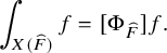
In particular, the double forest polynomials
$\mathfrak {P}_{F}(\textbf {x}_{n}; \textbf {t}_{n})$
 are Kronecker dual to the homology basis
$[X(F)]$
are Kronecker dual to the homology basis
$[X(F)]$
 of
$H^{\bullet }_{T_{n}}(\mathrm {QFl}_{n})$
of
$H^{\bullet }_{T_{n}}(\mathrm {QFl}_{n})$
 given in Corollary 11.6.
Proof. By Theorem 12.9, we have that for
$A\subset [n]$
 and
$\widehat {F} = \widehat {G} \cdot \mathsf {x}_{i} \in \operatorname {BNestFor}_{n-|A|}$
and
$\widehat {F} = \widehat {G} \cdot \mathsf {x}_{i} \in \operatorname {BNestFor}_{n-|A|}$
 , we have

after which the theorem follows recursively from the definition of
$[\Phi _{\widehat {F}}]$
 ; see [Reference Bergeron, Gagnon, Nadeau, Spink and Tewari6, §10] for more details on applying these operators to double forest polynomials.
Example 12.13. Let
$\Omega =\mathsf {r}_{1}^{-}\mathsf {r}_{1}^{+}\mathsf {e}_{2}\mathsf {e}_{1}\mathsf {r}_{2}^+\mathsf {e}_{3}$
 . Then

A polynomial
$a(\textbf {t}_{n})\in \mathbb Z[\textbf {t}_{n}]$
 is called
$\color {blue}{{Graham{-}positive}}$
is called
$\color {blue}{{Graham{-}positive}}$
 if it lies in
$\mathbb Z_{\geq 0}[t_2-t_1,\dots , t_{n} - t_{n-1}]$
if it lies in
$\mathbb Z_{\geq 0}[t_2-t_1,\dots , t_{n} - t_{n-1}]$
 . As shown by Graham [Reference Graham26], for any T-invariant subvariety
$X\subset \mathrm {Fl}_{n}$
. As shown by Graham [Reference Graham26], for any T-invariant subvariety
$X\subset \mathrm {Fl}_{n}$
 , the decomposition

into Schubert cycles has Graham-positive coefficients
$a_w(\textbf {t}_{n})=\int _X\mathfrak {S}_{w}(\textbf {x}_n;\textbf {t}_n)$
 . The Graham-positivity of
$[\Phi _{\widehat {F}}]\mathfrak {S}_{w}(\textbf {x}_n;\textbf {t}_n)$
. The Graham-positivity of
$[\Phi _{\widehat {F}}]\mathfrak {S}_{w}(\textbf {x}_n;\textbf {t}_n)$
 was shown through purely combinatorial means in [Reference Bergeron, Gagnon, Nadeau, Spink and Tewari6, Theorem 11.4], which we can now interpret geometrically.
Corollary 12.14 [Reference Bergeron, Gagnon, Nadeau, Spink and Tewari6, Theorem 11.4]
For
$F \in \operatorname {\mathsf {Forest}}_{n}$
 , the coefficient

is Graham-positive.
Remark 12.15. In [Reference Bergeron, Gagnon, Nadeau, Spink and Tewari6, Theorem 11.6] we also show that the product of two double forest polynomials has a Graham-positive expansion as a sum of double forest polynomials for combinatorial reasons. While the analogous result for double Schubert polynomials has a geometric explanation due to Graham [Reference Graham26], we do not have a geometric explanation for this positivity. We also show in [Reference Bergeron, Gagnon, Nadeau, Spink and Tewari6, Theorem 11.4] that
$[\Phi _{\widehat {F}}]\mathfrak {P}_{G}(\textbf {x}_n;\textbf {t}_n)$
 is Graham-positive, and we also do not have a geometric explanation for this positivity.
A Double forest polynomials
The purpose of this appendix is to give an alternative description for the ideal
$\text{EQSym}_{n}^+$
 as the kernel of the map

Theorem A.1. We have
$\text{EQSym}_{n}^+ = \ker (\mathbf {ev}_{\operatorname {NC}})$
 and, as a consequence,

The proof appears at the end of the appendix.
Remark A.2. Theorem A.1 belongs to a family of results known as “Orbit Harmonics.” In [Reference Bergeron and Gagnon5], the first two authors show that
$\mathbb Q \otimes _{\mathbb Z} \text{QSCoinv}_{n}$
 is the associated graded of the coordinate ring for the set of noncrossing partitions, considered as points using one-line notation. Specializing
$t_{i} \mapsto i$
is the associated graded of the coordinate ring for the set of noncrossing partitions, considered as points using one-line notation. Specializing
$t_{i} \mapsto i$
 in Theorem A.1, we recover this result and find a new cohomological interpretation for it.
We begin by extending the definition of forest polynomials to a basis of the full polynomial ring
$\mathbb Z[\textbf {t}_{n}][\textbf {x}_{n}]$
 . First define

so that we identify two forests if they differ only by some number of trailing isolated leaves. There is an obvious bijection between the internal nodes of any two forests identified in this manner, so we can speak of the internal nodes of
$F \in \operatorname {\mathsf {Forest}}$
 without ambiguity. Say that an internal node v of
$F \in \operatorname {\mathsf {Forest}}$
without ambiguity. Say that an internal node v of
$F \in \operatorname {\mathsf {Forest}}$
 is
$\color {blue}{{terminal}}$
is
$\color {blue}{{terminal}}$
 if both of its children are leaves, and let

so that
$i \in \mathrm {LTer}(F)$
 if and only if
$F = G \cdot \mathsf {e}_{i}$
if and only if
$F = G \cdot \mathsf {e}_{i}$
 for some
$G \in \operatorname {\mathsf {Forest}}$
for some
$G \in \operatorname {\mathsf {Forest}}$
 . We then define

We now consider double forest polynomials indexed by
$\mathrm {LTForest}_{n}$
 . Recall that as described in Remark 12.3, we have
$\mathfrak {P}_{F}(\textbf {x}_{m}; \textbf {t}_{m}) = \mathfrak {P}_{F \cdot (\mathsf {r}_{m+1}^{-})^{k}}(\textbf {x}_{m+k}; \textbf {t}_{m+k})$
. Recall that as described in Remark 12.3, we have
$\mathfrak {P}_{F}(\textbf {x}_{m}; \textbf {t}_{m}) = \mathfrak {P}_{F \cdot (\mathsf {r}_{m+1}^{-})^{k}}(\textbf {x}_{m+k}; \textbf {t}_{m+k})$
 for all
$m, k \ge 0$
for all
$m, k \ge 0$
 and
$F \in \operatorname {\mathsf {Forest}}_{m}$
and
$F \in \operatorname {\mathsf {Forest}}_{m}$
 . Thus each class
$F \in \mathrm {LTForest}_{n}$
. Thus each class
$F \in \mathrm {LTForest}_{n}$
 defines a unique forest polynomial in any set of x and t variables
$(\textbf {x}_{m}; \textbf {t}_{m})$
defines a unique forest polynomial in any set of x and t variables
$(\textbf {x}_{m}; \textbf {t}_{m})$
 such that
$m \ge \max \operatorname {supp}{F}$
such that
$m \ge \max \operatorname {supp}{F}$
 .
.
Definition A.3. For
$F \in \mathrm {LTForest}_{n}$
 , the
$\color {blue}{{n{-}truncated\, double\, forest\, polynomial}}$
, the
$\color {blue}{{n{-}truncated\, double\, forest\, polynomial}}$
 is defined to be

where the right-hand side is the specialization of the unique forest polynomial defined by F.
The truncated forest polynomials have the property that

for
$1 \le i \le n$
 , where
${\mathsf {E}_{1}}, \ldots , {\mathsf {E}_{n-1}}$
, where
${\mathsf {E}_{1}}, \ldots , {\mathsf {E}_{n-1}}$
 are as defined in Section 12.2 and

In [Reference Bergeron, Gagnon, Nadeau, Spink and Tewari6, Corollary 4.7 (2)] we show that

Thus, as a consequence, we obtain a
$\mathbb Z$
 -basis of
$\mathbb Z[\textbf {x}_{n}]$
-basis of
$\mathbb Z[\textbf {x}_{n}]$
 consisting of (single) forest polynomials

We prove in [Reference Bergeron, Gagnon, Nadeau, Spink and Tewari6, Corollary 4.6] that these are the same forest polynomials studied in [Reference Nadeau, Spink and Tewari39, Reference Nadeau and Tewari41].
Theorem A.4 [Reference Nadeau, Spink and Tewari39, Theorem 9.7], [Reference Nadeau and Tewari41, Theorem 3.7]
The forest polynomials
$\mathfrak {P}_{F}(\textbf {x}_n;0)$
 with
$F \in \mathrm {LTForest}_{n}$
with
$F \in \mathrm {LTForest}_{n}$
 and
$n \in \mathrm {LTer}(F)$
and
$n \in \mathrm {LTer}(F)$
 are a
$\mathbb Z$
are a
$\mathbb Z$
 -basis for
$\text{QSym}_{n}^+$
-basis for
$\text{QSym}_{n}^+$
 .
.
We also define the set of
$\color {blue}{{zigzag\, forests}}$
 to be
to be

The
$\mathfrak {P}_{F}(\textbf {x}_{n}; \textbf {t}_{n})$
 for
$F \in \mathsf{ZigZag}_{n}$
for
$F \in \mathsf{ZigZag}_{n}$
 are called
$\color {blue}{{double\, fundamental\, quasisymmetric\, polynomials}}$
are called
$\color {blue}{{double\, fundamental\, quasisymmetric\, polynomials}}$
 , and in [Reference Bergeron, Gagnon, Nadeau, Spink and Tewari6, §4 and §7] we show that they form a basis for
$\text{EQSym}_{n}$
, and in [Reference Bergeron, Gagnon, Nadeau, Spink and Tewari6, §4 and §7] we show that they form a basis for
$\text{EQSym}_{n}$
 . Via [Reference Nadeau, Spink and Tewari39], [Reference Bergeron, Gagnon, Nadeau, Spink and Tewari6] also show that the
$\mathfrak {P}_{F}(\textbf {x}_{n}; 0)$
. Via [Reference Nadeau, Spink and Tewari39], [Reference Bergeron, Gagnon, Nadeau, Spink and Tewari6] also show that the
$\mathfrak {P}_{F}(\textbf {x}_{n}; 0)$
 are the classical fundamental quasisymmetric basis for
$\text{QSym}_{n}$
are the classical fundamental quasisymmetric basis for
$\text{QSym}_{n}$
 .
.
Proof of Theorem A.1
Theorem 11.11 shows that

so we only need to show that
$\text{EQSym}_{n}^+ = \ker (\mathbf {ev}_{\operatorname {NC}})$
 . By (A.2), it suffices to show the inclusions

For the second inclusion in Equation (A.3) we use the fact, proved in [Reference Bergeron, Gagnon, Nadeau, Spink and Tewari6, Theorem 7.1], that if
$f(\textbf {x}_n;\textbf {t}_n)\in \text{EQSym}_{n}$
 then
$\operatorname {ev}_{w}f=\operatorname {ev}_{\operatorname {id}}f$
then
$\operatorname {ev}_{w}f=\operatorname {ev}_{\operatorname {id}}f$
 for all
$w \in \operatorname {NC}_n$
for all
$w \in \operatorname {NC}_n$
 , so clearly

We now establish the first inclusion by showing that for all
$F \in \mathrm {LTForest}_{n}\setminus \operatorname {\mathsf {Forest}}_n$
 we have
$\mathfrak {P}_{F}(\textbf {x}_n;\textbf {t}_n) \in \text{EQSym}_{n}^+$
we have
$\mathfrak {P}_{F}(\textbf {x}_n;\textbf {t}_n) \in \text{EQSym}_{n}^+$
 . We proceed by induction on
$|F|$
. We proceed by induction on
$|F|$
 . Our base case is
$|F|=1$
. Our base case is
$|F|=1$
 , wherein the assumption
$n \in \mathrm {LTer}(T)$
, wherein the assumption
$n \in \mathrm {LTer}(T)$
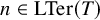 implies that
$F = (\mathsf {r}_{1}^{-})^{n-1}\cdot \mathsf {e}_{n}$
implies that
$F = (\mathsf {r}_{1}^{-})^{n-1}\cdot \mathsf {e}_{n}$
 , so that
$\mathfrak {P}_{F}(\textbf {x}_n;\textbf {t}_n) \in \text{EQSym}_{n}$
, so that
$\mathfrak {P}_{F}(\textbf {x}_n;\textbf {t}_n) \in \text{EQSym}_{n}$
 as
$F\in \mathsf{ZigZag}_{n}$
as
$F\in \mathsf{ZigZag}_{n}$
 (alternatively as
$\mathfrak {P}_{F}(\textbf {x}_n;\textbf {t}_n)=x_1+\cdots +x_n-t_1-\cdots -t_n$
(alternatively as
$\mathfrak {P}_{F}(\textbf {x}_n;\textbf {t}_n)=x_1+\cdots +x_n-t_1-\cdots -t_n$
 ).
).
Now assume that
$|F|> 1$
 . By [Reference Nadeau, Spink and Tewari39, Theorem 9.7], the (single) forest polynomial
$\mathfrak {P}_{F}(\textbf {x}_n)$
. By [Reference Nadeau, Spink and Tewari39, Theorem 9.7], the (single) forest polynomial
$\mathfrak {P}_{F}(\textbf {x}_n)$
 lies in
$\text{QSym}_{n}^+$
lies in
$\text{QSym}_{n}^+$
 , which is generated by the fundamental quasisymmetric polynomials
$\mathfrak {P}_{G}(\textbf {x}_n)$
, which is generated by the fundamental quasisymmetric polynomials
$\mathfrak {P}_{G}(\textbf {x}_n)$
 for
$\varnothing \ne G \in \mathsf{ZigZag}_{n}$
for
$\varnothing \ne G \in \mathsf{ZigZag}_{n}$
 . One may then write

As the double fundamental quasisymmetric polynomial
$\mathfrak {P}_{G}(\textbf {x}_n;\textbf {t}_n)$
 lies in
$\text{EQSym}_{n}^+$
lies in
$\text{EQSym}_{n}^+$
 for
$\varnothing \neq G\in \mathsf{ZigZag}_{n}$
for
$\varnothing \neq G\in \mathsf{ZigZag}_{n}$
 , the difference

can be written as a
$\mathbb Z[\textbf {t}_{n}]$
 -linear combination of double forest polynomials
$\mathfrak {P}_{H}(\textbf {x}_n; \textbf {t}_{n})$
-linear combination of double forest polynomials
$\mathfrak {P}_{H}(\textbf {x}_n; \textbf {t}_{n})$
 with
$H\in \mathrm {LTForest}_{n}\setminus \operatorname {\mathsf {Forest}}_n$
with
$H\in \mathrm {LTForest}_{n}\setminus \operatorname {\mathsf {Forest}}_n$
 . Furthermore, the difference (A.4) contains no monomials consisting entirely of x-variables, so each H must have
$|H| < |F|$
. Furthermore, the difference (A.4) contains no monomials consisting entirely of x-variables, so each H must have
$|H| < |F|$
 . By induction, we have now expressed
$\mathfrak {P}_{F}(\textbf {x}_n;\textbf {t}_n)$
. By induction, we have now expressed
$\mathfrak {P}_{F}(\textbf {x}_n;\textbf {t}_n)$
 as an element of
$\text{EQSym}_{n}^+$
as an element of
$\text{EQSym}_{n}^+$
 , completing the proof.
Acknowledgments
We are very grateful to Allen Knutson and Alex Fink for numerous helpful conversations and their generous sharing of ideas. VT owes a lot to enlightening conversations with Dave Anderson. Thanks also go out to Sara Billey, Alexander Woo, and Alejandro Morales for pointers to relevant results in the literature. Finally, we thank the referees for their insightful feedback.
Competing interests
The authors have no competing interests to declare.
Funding statement
NB and LG were supported by the Natural Sciences and Engineering Research Council of Canada (NSERC) and York Research Chair in Applied Algebra. PN was partially supported by French ANR grant ANR-19-CE48-0011 (COMBINÉ). HS and VT acknowledge the support of the NSERC [RGPIN-2024-04181] and [RGPIN-2024-05433], respectively.


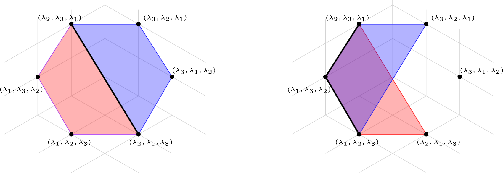






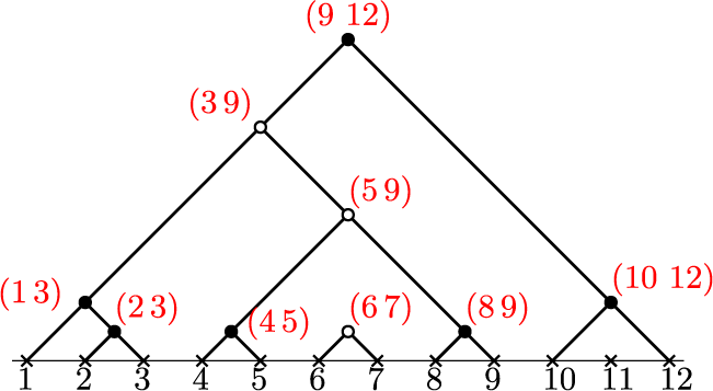


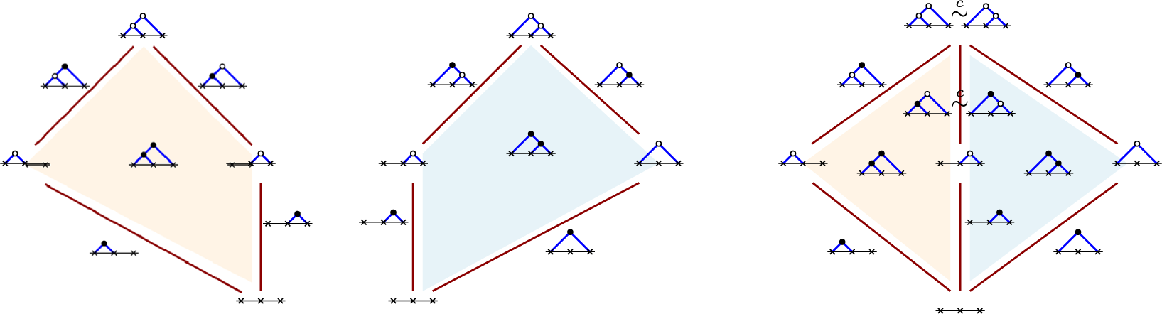


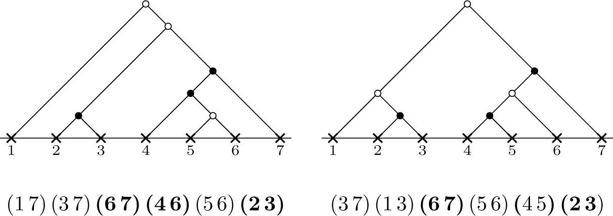

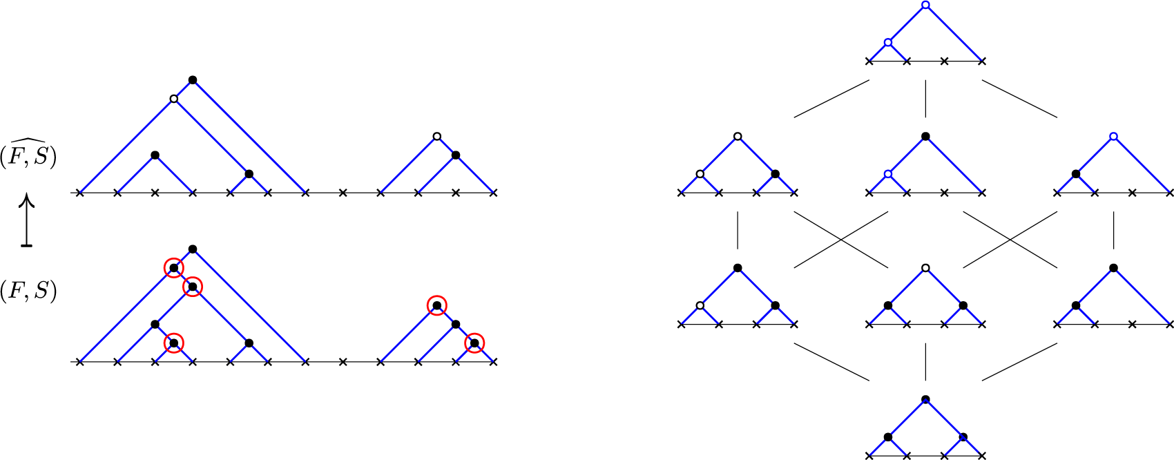


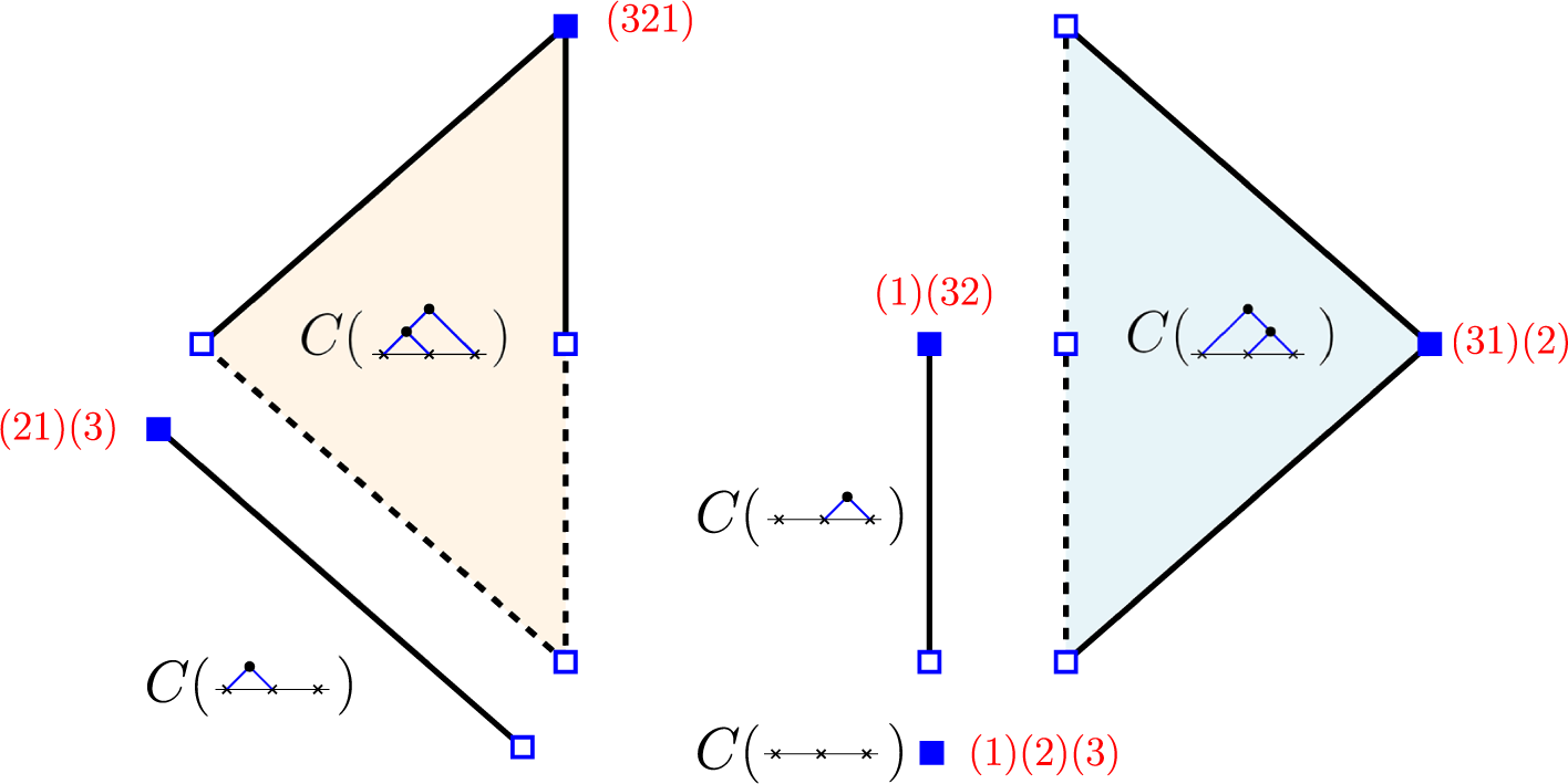


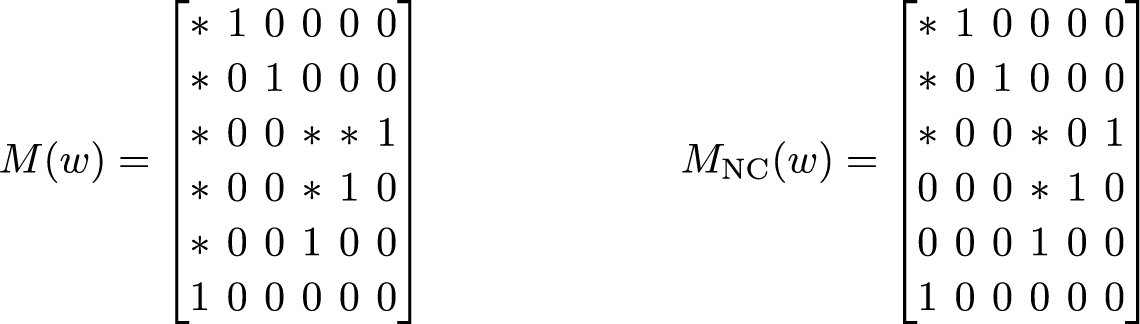

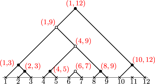
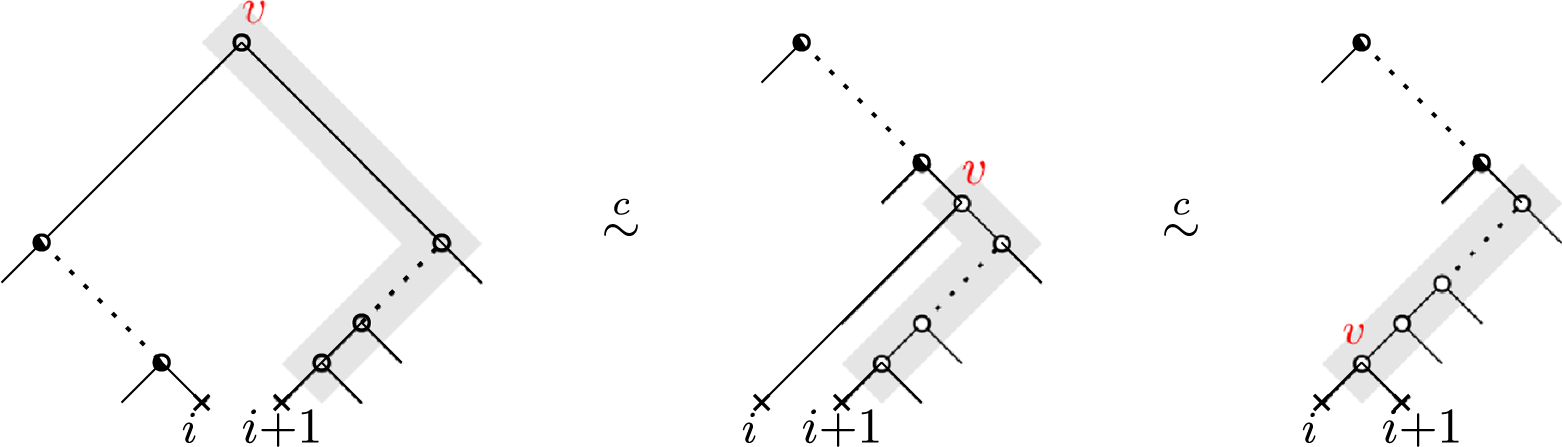
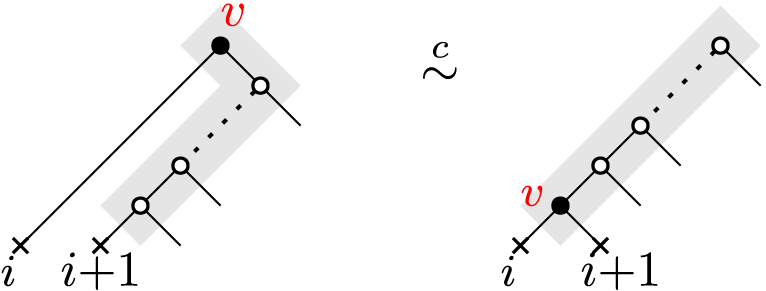
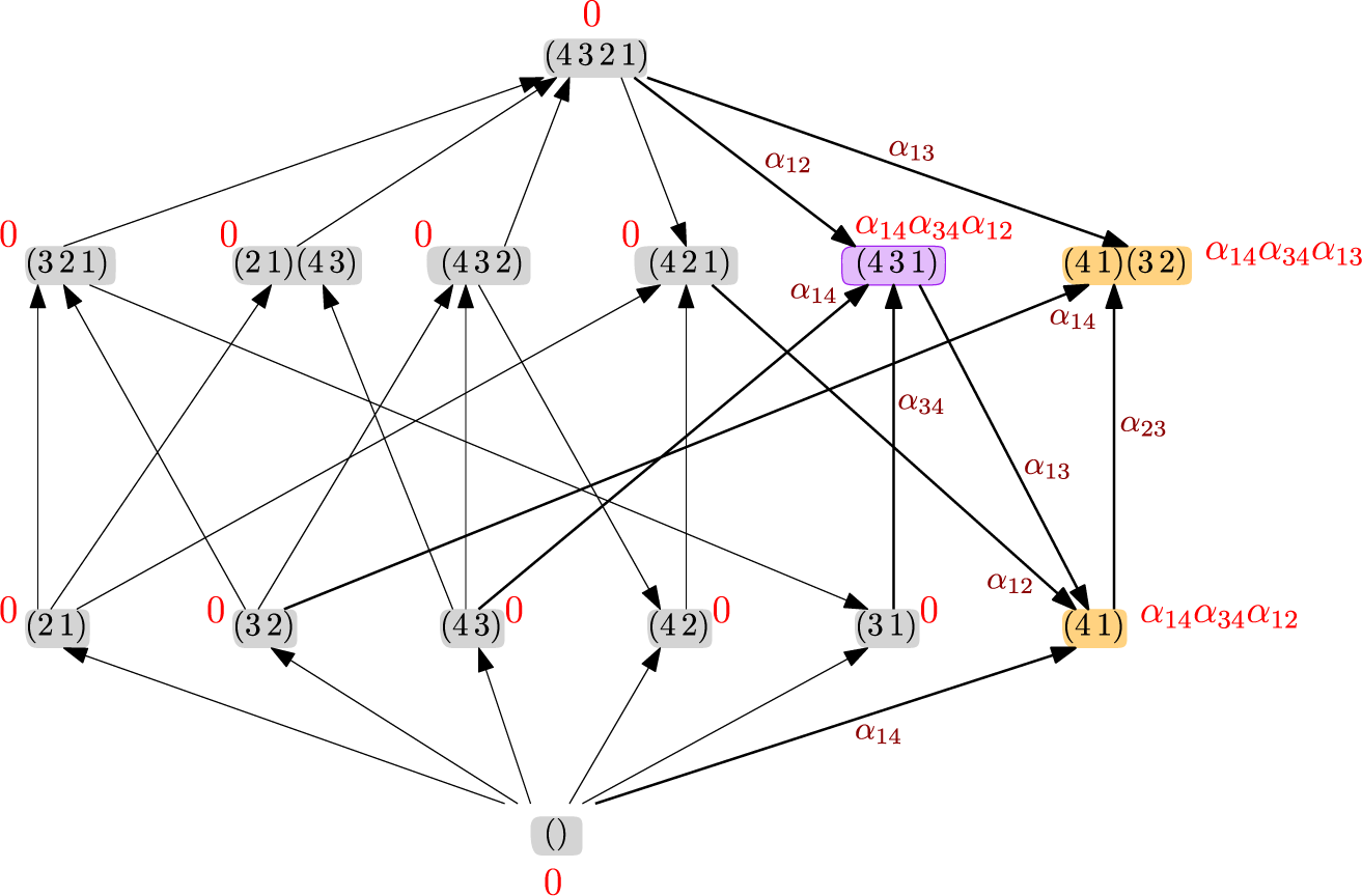


 Open access

