


1 Introduction
Increasing energy efficiency by reducing aerodynamic drag is a challenging task for the design and manufacture of future aircraft, wind turbines and turbomachinery. An approach to enhance the aerodynamic efficiency is to extend the regions of laminar boundary-layer flow on the aerodynamic surfaces (laminar flow control) to reduce the skin-friction drag.
On swept aircraft wings and turbomachinery/wind-turbine blades a three-dimensional boundary-layer flow develops due to the chordwise acceleration/deceleration of the flow. Inside the boundary layer a crossflow (CF) velocity component perpendicular to the local potential-flow direction arises. The CF velocity profile is inflectional, causing an inviscid instability and as a consequence exponential amplification of both steady and travelling CF-vortex modes. At low free-stream turbulence conditions as in free flight, steady CF vortices are most efficiently forced by surface roughness and prevail in the linear and nonlinear stages of transition. The amplification rates of travelling modes are higher than those of steady modes, and travelling CF vortices dominate in environments with non-negligible free-stream turbulence conditions, for example in turbomachinery and wind-turbine applications or in cases with other unsteady excitation. Steady or travelling CF vortices generate localized high-shear layers and trigger a (co-running) strong secondary instability, causing rapid transition to turbulence. For details of CF-vortex-induced transition, see e.g. Bippes (Reference Bippes1999), Wassermann & Kloker (Reference Wassermann and Kloker2002), Saric, Reed & White (Reference Saric, Reed and White2003), Wassermann & Kloker (Reference Wassermann and Kloker2003), Downs & White (Reference Downs and White2013), Li et al. (Reference Li, Choudhari, Duan and Chang2014), Serpieri & Kotsonis (Reference Serpieri and Kotsonis2016) or Borodulin, Ivanov & Kachanov (Reference Borodulin, Ivanov and Kachanov2017).
In laminar flow control, a significant delay of transition can be achieved by a reduction of the basic CF velocity using slot-panel or hole-panel suction systems. Detailed overviews of experiments and flight campaigns are given by Joslin (Reference Joslin1998a ,Reference Joslin b ); see Messing & Kloker (Reference Messing and Kloker2010) for a summary. Saric, Carrillo & Reibert (Reference Saric, Carrillo and Reibert1998) proposed another method using distributed roughness elements. A spanwise row of regularly distributed roughness elements is employed to excite steady ‘subcritical’ CF-vortex modes that are spaced more narrowly than the integrally most amplified mode. Without causing significant secondary instability, the resulting steady, narrowly spaced CF vortices induce a beneficial mean-flow distortion and hinder the growth of the naturally most amplified modes. Hence, transition to turbulence is delayed. The applicability of the technique to control transition induced by complex disturbance fields that include both steady and travelling primary disturbances was shown by Hosseini et al. (Reference Hosseini, Tempelmann, Hanifi and Henningson2013). The same concept, however named upstream flow deformation (UFD) and not necessarily based on roughness elements, was proposed by Wassermann & Kloker (Reference Wassermann and Kloker2002) using direct numerical simulations (DNS). Their detailed analysis showed that the three-dimensional part of the control vortices weakens mainly the receptivity, whereas the mean-flow distortion reduces the growth rate of amplified modes. Recently, this approach was implemented in an experiment by Lohse, Barth & Nitsche (Reference Lohse, Barth and Nitsche2016) employing pneumatic actuators with either weak steady suction or blowing. Further experimental investigations were performed by Borodulin et al. (Reference Borodulin, Ivanov, Kachanov and Hanifi2016) using complementary excitation of an acoustic field in addition to distributed roughness elements and by Ivanov, Mischenko & Ustinov (Reference Ivanov, Mischenko and Ustinov2018) using rows of oblique surface non-uniformities.
Interest in the application of plasma actuators for laminar flow control emerged in the last decade. The alternating-current dielectric-barrier-discharge plasma actuator is the most frequently used actuator type. Operated in a quasi-steady fashion without modulation of the high-frequency driving, it generates a steady volume force that locally accelerates the surrounding fluid, whereas unsteady operation with driving-frequency modulation can excite (anti-phased) control disturbances of appropriate frequency. Further details of the actuators’ working principle and ongoing research are provided in recent overview articles, see e.g. Benard & Moreau (Reference Benard and Moreau2014), Kotsonis (Reference Kotsonis2015) and Kriegseis, Simon & Grundmann (Reference Kriegseis, Simon and Grundmann2016). Most of the works on laminar flow control focused on two-dimensional, spanwise symmetric boundary-layer flows. Various control approaches were applied, such as (i) the stabilization of the (longitudinal) velocity profile, see e.g. Grundmann & Tropea (Reference Grundmann and Tropea2007), Riherd & Roy (Reference Riherd and Roy2013), Dörr & Kloker (Reference Dörr and Kloker2015a ), (ii) the active cancellation of Tollmien–Schlichting waves, see e.g. Grundmann & Tropea (Reference Grundmann and Tropea2008), Kotsonis et al. (Reference Kotsonis, Giepmann, Hulshoff and Veldhuis2013), (iii) the damping of boundary-layer streaks, see Hanson et al. (Reference Hanson, Bade, Belson, Lavoie, Naguib and Rowley2014), Riherd & Roy (Reference Riherd and Roy2014), or (iv) the spanwise modulation of the flow field, see Barckmann, Tropea & Grundmann (Reference Barckmann, Tropea and Grundmann2015), Dörr & Kloker (Reference Dörr and Kloker2018).
Three-dimensional boundary-layer control using plasma actuators began more recently. Schuele, Corke & Matlis (Reference Schuele, Corke and Matlis2013) and Serpieri, Yadala Venkata & Kotsonis (Reference Serpieri, Yadala Venkata and Kotsonis2017) excited ‘subcritical’ CF-vortex control modes by a spanwise row of plasma actuators in experiments; however, no conclusive transition delay has been reported so far with three-dimensional actuators. Note that the dielectric-barrier-discharge plasma actuators used seem to cause an unsteady low-frequency component in the flow, even if the driving frequency has been chosen high enough to lie outside the primarily amplified frequency range (cf. Serpieri et al. Reference Serpieri, Yadala Venkata and Kotsonis2017). A low-frequency component is negligible for Tollmien–Schlichting instability but not for CF instability. Applying DNS, successful delay of transition induced by steady CF vortices employing the UFD technique was achieved by Dörr & Kloker (Reference Dörr and Kloker2017) using ‘classical’ plasma actuators; Shahriari, Kollert & Hanifi (Reference Shahriari, Kollert and Hanifi2018) investigated ring-type plasma actuators based on the work by Choi & Kim (Reference Choi and Kim2018). Note that both DNS studies were based on steady volume-force models. Similar to the application of homogeneous suction, Dörr & Kloker (Reference Dörr and Kloker2015b ) and Chernyshev et al. (Reference Chernyshev, Gamirullin, Khomich, Kuryachii, Litinov, Manuilovich, Moshkunov, Rebrov, Rusyanov and Yamshchikov2016) numerically investigated plasma actuators to stabilize a three-dimensional boundary-layer flow by base-flow manipulation: the plasma actuators are then used to reduce the basic CF velocity and hence the growth of both steady and unsteady primary CF instabilities. Recently, Yadala et al. (Reference Yadala, Hehner, Serpieri, Benard, Dörr, Kloker and Kotsonis2018) showed the success of this approach employing two-dimensional plasma actuators in experiments. Akin to the pinpoint-suction concept (Friederich & Kloker Reference Friederich and Kloker2012), Dörr & Kloker (Reference Dörr and Kloker2016) demonstrated that three-dimensional plasma actuators can be used to directly attenuate nonlinear steady CF vortices. Positioning the actuators at selected spanwise positions to weaken oncoming vortices and thus the connected secondary instability, transition to turbulence is delayed; see also the work of Wang, Wang & Fu (Reference Wang, Wang and Fu2017) who followed up the investigations by Dörr & Kloker (Reference Dörr and Kloker2016).
In the current work the potential of plasma actuators operated unsteadily at low frequency is investigated to control the CF-induced transition. Travelling CF-vortex modes have not been considered so far as subcritical control modes for UFD, and here the physical mechanisms of this approach are scrutinized. Effects of single travelling control modes, excited by blowing/suction, on the flow instabilities are investigated at first. Based on the findings from this fundamental study, an effective configuration using plasma-actuator volume forcing is designed to control transition induced by both steady or travelling CF vortices. The investigated base flow resembles the redesigned DLR-Göttingen swept flat-plate experiment, a model flow for the three-dimensional boundary-layer flow as it develops in the front region on the upper side of a swept wing; see Lohse et al. (Reference Lohse, Barth and Nitsche2016) and Barth, Hein & Rosemann (Reference Barth, Hein and Rosemann2017) for further details of the set-up of the base flow.
The paper is structured as follows: § 2 describes the numerical set-up. Base-flow characteristics and reference cases are presented in § 3. In § 4, the UFD method using travelling control modes is discussed in detail.
2 Numerical set-up
2.1 Basic set-up
Integration domain and coordinate systems.
The DNS are performed with our compressible, high-order, finite-difference code NS3D; see e.g. Dörr & Kloker (Reference Dörr and Kloker2015b
) for details. The vector
 $\boldsymbol{u}=[u,v,w]^{\text{T}}$
denotes the velocity components in the chordwise, wall-normal and spanwise directions
$\boldsymbol{u}=[u,v,w]^{\text{T}}$
denotes the velocity components in the chordwise, wall-normal and spanwise directions
 $x$
,
$x$
,
 $y$
and
$y$
and
 $z$
, respectively. Velocities and length scales are normalized by the chordwise reference velocity
$z$
, respectively. Velocities and length scales are normalized by the chordwise reference velocity
 $\bar{U}_{\infty }$
and the reference length
$\bar{U}_{\infty }$
and the reference length
 $\bar{L}$
, respectively, with the overbar denoting dimensional values; further, the reference density is
$\bar{L}$
, respectively, with the overbar denoting dimensional values; further, the reference density is
 $\bar{\unicode[STIX]{x1D70C}}_{\infty }$
and the reference temperature
$\bar{\unicode[STIX]{x1D70C}}_{\infty }$
and the reference temperature
 $\bar{T}_{\infty }$
. In the experiments the Mach number based on the chordwise free-stream velocity
$\bar{T}_{\infty }$
. In the experiments the Mach number based on the chordwise free-stream velocity
 $\bar{U}_{\infty ,exp}=22.66~\text{m}~\text{s}^{-1}$
is
$\bar{U}_{\infty ,exp}=22.66~\text{m}~\text{s}^{-1}$
is
 $Ma_{\infty ,exp}=0.066$
. The reference length is defined as
$Ma_{\infty ,exp}=0.066$
. The reference length is defined as
 $\bar{L}_{exp}=0.1~\text{m}$
. For the simulations a computationally non-prohibitive Mach number
$\bar{L}_{exp}=0.1~\text{m}$
. For the simulations a computationally non-prohibitive Mach number
 $Ma_{\infty }=0.2$
is chosen, keeping the ambient conditions and the Reynolds number range identical. The reference values in the simulations are then
$Ma_{\infty }=0.2$
is chosen, keeping the ambient conditions and the Reynolds number range identical. The reference values in the simulations are then
 $\bar{U}_{\infty }=68.871~\text{m}~\text{s}^{-1}$
,
$\bar{U}_{\infty }=68.871~\text{m}~\text{s}^{-1}$
,
 $\bar{L}=0.033~\text{m}$
,
$\bar{L}=0.033~\text{m}$
,
 $\bar{\unicode[STIX]{x1D70C}}_{\infty }=1.181~\text{kg}~\text{m}^{-3}$
and
$\bar{\unicode[STIX]{x1D70C}}_{\infty }=1.181~\text{kg}~\text{m}^{-3}$
and
 $\bar{T}_{\infty }=\bar{T}_{wall}=295.0~\text{K}$
. For details of the base-flow generation for the DNS, see Dörr & Kloker (Reference Dörr and Kloker2017); note that the reference length
$\bar{T}_{\infty }=\bar{T}_{wall}=295.0~\text{K}$
. For details of the base-flow generation for the DNS, see Dörr & Kloker (Reference Dörr and Kloker2017); note that the reference length
 $\bar{L}_{exp}$
is not the length of the plate
$\bar{L}_{exp}$
is not the length of the plate
 $\bar{L}_{plate,exp}=0.6~\text{m}$
in the experiments.
$\bar{L}_{plate,exp}=0.6~\text{m}$
in the experiments.
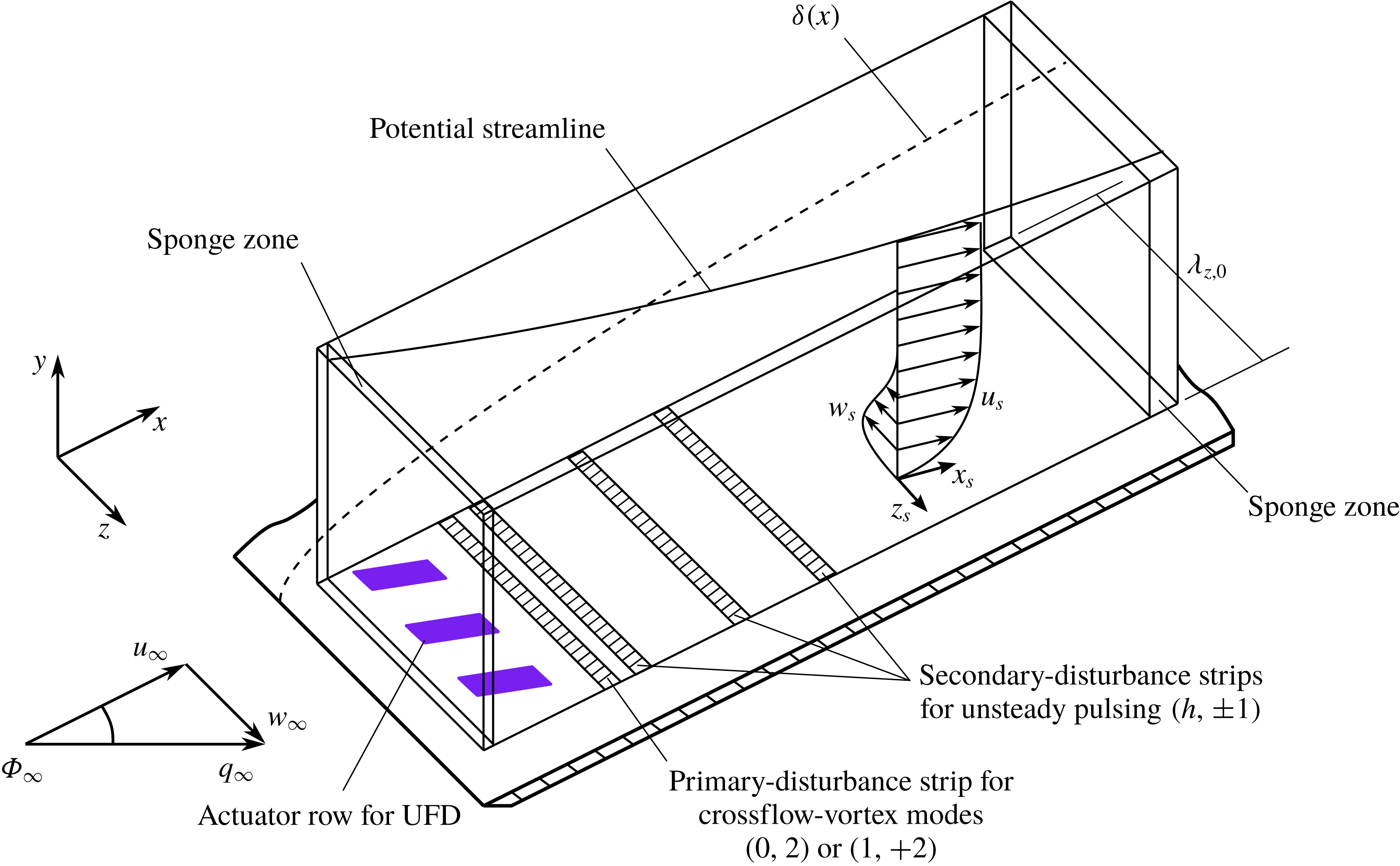
A rectangular integration domain with a block-structured Cartesian grid is considered for the simulations (see figure 1). The inflow and outflow are treated with characteristic boundary conditions. In addition, sponge layers based on a volume-forcing term and a spatial compact tenth-order low-pass filter are employed to further minimize disturbances. To allow mass flow through the free-stream boundary for the simulations including the plasma actuators, the conditions there are as follows: the base-flow values for
 $\unicode[STIX]{x1D70C}$
and
$\unicode[STIX]{x1D70C}$
and
 $T$
are kept and
$T$
are kept and
 $\text{d}u/\text{d}y|_{e}=\text{d}w/\text{d}y|_{e}=0$
allows
$\text{d}u/\text{d}y|_{e}=\text{d}w/\text{d}y|_{e}=0$
allows
 $u_{e}$
and
$u_{e}$
and
 $w_{e}$
to adapt, where the subscript
$w_{e}$
to adapt, where the subscript
 $e$
denotes the values at the upper boundary of the domain; in addition,
$e$
denotes the values at the upper boundary of the domain; in addition,
 $v_{e}$
is calculated according to
$v_{e}$
is calculated according to
 $\text{d}v/\text{d}y|_{e}=-(\text{d}(\unicode[STIX]{x1D70C}_{e}u_{e})/\text{d}x+\text{d}(\unicode[STIX]{x1D70C}_{e}w_{e})/\text{d}z)/\unicode[STIX]{x1D70C}_{e}$
, assuming
$\text{d}v/\text{d}y|_{e}=-(\text{d}(\unicode[STIX]{x1D70C}_{e}u_{e})/\text{d}x+\text{d}(\unicode[STIX]{x1D70C}_{e}w_{e})/\text{d}z)/\unicode[STIX]{x1D70C}_{e}$
, assuming
 $\text{d}\unicode[STIX]{x1D70C}/\text{d}y|_{e}=0$
. For more details, see Dörr & Kloker (Reference Dörr and Kloker2016). At the lateral boundaries periodicity conditions are prescribed. The fundamental spanwise wavelength is
$\text{d}\unicode[STIX]{x1D70C}/\text{d}y|_{e}=0$
. For more details, see Dörr & Kloker (Reference Dörr and Kloker2016). At the lateral boundaries periodicity conditions are prescribed. The fundamental spanwise wavelength is
 $\unicode[STIX]{x1D706}_{z,0}=0.180$
, corresponding to the fundamental spanwise wavenumber
$\unicode[STIX]{x1D706}_{z,0}=0.180$
, corresponding to the fundamental spanwise wavenumber
 $\unicode[STIX]{x1D6FE}_{0}=2\unicode[STIX]{x03C0}/\unicode[STIX]{x1D706}_{z,0}=35.0$
. Explicit finite differences of eighth order are used for the discretization in the
$\unicode[STIX]{x1D6FE}_{0}=2\unicode[STIX]{x03C0}/\unicode[STIX]{x1D706}_{z,0}=35.0$
. Explicit finite differences of eighth order are used for the discretization in the
 $x$
-direction and
$x$
-direction and
 $y$
-direction, and a Fourier spectral ansatz is used for the
$y$
-direction, and a Fourier spectral ansatz is used for the
 $z$
-direction. In the chordwise direction
$z$
-direction. In the chordwise direction
 $x$
, an equally spaced grid with 2604 points is used, covering
$x$
, an equally spaced grid with 2604 points is used, covering
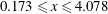 $0.173\leqslant x\leqslant 4.078$
, with
$0.173\leqslant x\leqslant 4.078$
, with
 $\unicode[STIX]{x0394}x=1.5\times 10^{-3}$
. In the wall-normal direction
$\unicode[STIX]{x0394}x=1.5\times 10^{-3}$
. In the wall-normal direction
 $y$
, a stretched grid with 152 points is employed,
$y$
, a stretched grid with 152 points is employed,
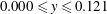 $0.000\leqslant y\leqslant 0.121$
, with
$0.000\leqslant y\leqslant 0.121$
, with
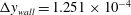 $\unicode[STIX]{x0394}y_{wall}=1.251\times 10^{-4}$
and
$\unicode[STIX]{x0394}y_{wall}=1.251\times 10^{-4}$
and
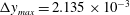 $\unicode[STIX]{x0394}y_{max}=2.135\times 10^{-3}$
. The fundamental spanwise wavelength
$\unicode[STIX]{x0394}y_{max}=2.135\times 10^{-3}$
. The fundamental spanwise wavelength
 $\unicode[STIX]{x1D706}_{z,0}$
is discretized with 64 points (
$\unicode[STIX]{x1D706}_{z,0}$
is discretized with 64 points (
 $K=21$
de-aliased Fourier modes), yielding
$K=21$
de-aliased Fourier modes), yielding
 $\unicode[STIX]{x0394}z=2.805\times 10^{-3}$
. An explicit fourth-order Runge–Kutta scheme is employed for the time integration. The fundamental angular frequency is
$\unicode[STIX]{x0394}z=2.805\times 10^{-3}$
. An explicit fourth-order Runge–Kutta scheme is employed for the time integration. The fundamental angular frequency is
 $\unicode[STIX]{x1D714}_{0}=6.0$
, and the time step is
$\unicode[STIX]{x1D714}_{0}=6.0$
, and the time step is
 $\unicode[STIX]{x0394}t=8.727\times 10^{-6}$
.
$\unicode[STIX]{x0394}t=8.727\times 10^{-6}$
.
A disturbance strip at the wall with synthetic blowing and suction, centred at
 $x=0.800$
,
$x=0.800$
,
 $0.766\leqslant x\leqslant 0.835$
, and alternating in spanwise direction
$0.766\leqslant x\leqslant 0.835$
, and alternating in spanwise direction
 $z$
, is employed to excite the primary CF vortex disturbances
$z$
, is employed to excite the primary CF vortex disturbances
 $(0,2)$
or
$(0,2)$
or
 $(1,+2)$
; the double-spectral notation (
$(1,+2)$
; the double-spectral notation (
 $h\unicode[STIX]{x1D714}_{0}$
,
$h\unicode[STIX]{x1D714}_{0}$
,
 $k\unicode[STIX]{x1D6FE}_{0}$
) is used. To initiate controlled laminar breakdown, two additional disturbance strips are positioned farther downstream to excite pulse-like (background) disturbances (
$k\unicode[STIX]{x1D6FE}_{0}$
) is used. To initiate controlled laminar breakdown, two additional disturbance strips are positioned farther downstream to excite pulse-like (background) disturbances (
 $h,\pm 1$
), with
$h,\pm 1$
), with
 $h=1{-}50$
. The disturbances are forced near
$h=1{-}50$
. The disturbances are forced near
 $x=1.0$
,
$x=1.0$
,
 $x=2.0$
and
$x=2.0$
and
 $x=2.5$
with a strip extension of 0.045, respectively. Note that the modes
$x=2.5$
with a strip extension of 0.045, respectively. Note that the modes
 $|k|\geqslant 2$
are nonlinearly generated at once by the primary modes.
$|k|\geqslant 2$
are nonlinearly generated at once by the primary modes.
2.2 Modelling of the plasma actuator
(a) Schematic of plasma actuator and planar volume-force distribution. (b) Angle
 $\unicode[STIX]{x1D6FD}_{PA}$
for rotation about the wall-normal axis
$\unicode[STIX]{x1D6FD}_{PA}$
for rotation about the wall-normal axis
 $y$
; see Dörr & Kloker (Reference Dörr and Kloker2017).
$y$
; see Dörr & Kloker (Reference Dörr and Kloker2017).
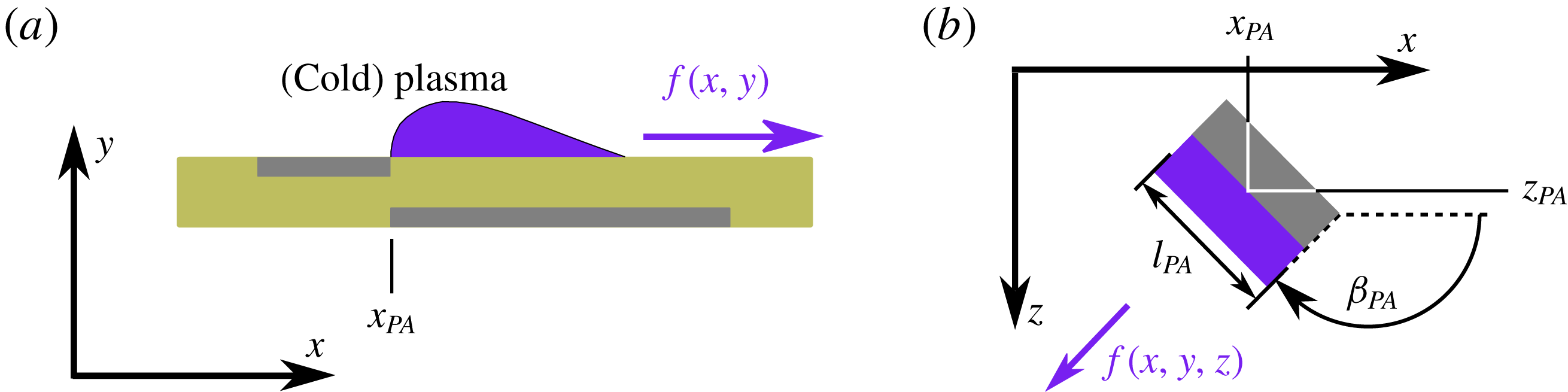
Based on the empirical model given by Maden et al. (Reference Maden, Maduta, Kriegseis, Jakirlić, Schwarz, Grundmann and Tropea2013), a non-dimensional wall-parallel volume-force distribution
 $f(x,y)$
in the plane perpendicular to the electrode axis is prescribed. The three-dimensional distribution of the volume force
$f(x,y)$
in the plane perpendicular to the electrode axis is prescribed. The three-dimensional distribution of the volume force
 $f(x,y,z)$
produced by a plasma actuator with electrode length
$f(x,y,z)$
produced by a plasma actuator with electrode length
 $l_{PA}$
is then modelled by extrusion of
$l_{PA}$
is then modelled by extrusion of
 $f(x,y)$
along the electrode axis, as sketched in figure 2. At the lateral edges a fifth-order polynomial is imposed over a range of 10 % of the electrode length to smooth the changeover from zero to maximum forcing. The angle
$f(x,y)$
along the electrode axis, as sketched in figure 2. At the lateral edges a fifth-order polynomial is imposed over a range of 10 % of the electrode length to smooth the changeover from zero to maximum forcing. The angle
 $\unicode[STIX]{x1D6FD}_{PA}$
defines the clockwise rotation of the actuator about the wall-normal axis through
$\unicode[STIX]{x1D6FD}_{PA}$
defines the clockwise rotation of the actuator about the wall-normal axis through
 $(x_{PA},z_{PA})$
. According to previous investigations by Dörr & Kloker (Reference Dörr and Kloker2015b
) and Dörr & Kloker (Reference Dörr and Kloker2016), the effect of the wall-normal force component is negligible.
$(x_{PA},z_{PA})$
. According to previous investigations by Dörr & Kloker (Reference Dörr and Kloker2015b
) and Dörr & Kloker (Reference Dörr and Kloker2016), the effect of the wall-normal force component is negligible.
Based on the alternating-current operation of plasma actuators, an unsteady volume force with alternating direction (push and pull events with non-zero time mean) is inherently induced. If the frequency of the operating voltage is set clearly above the unstable frequency range of the boundary layer, the high-frequency unsteadiness can be neglected, and only the steady mean force resulting from the asymmetric push and pull events has to be taken into consideration. In the present study, in contrast, we simulate plasma actuators with low-frequency operation and make full use of the unsteady nature for the excitation of unsteady CF-vortex modes, resembling the direct-frequency mode for active wave cancellation investigated by Kurz et al. (Reference Kurz, Tropea, Grundmann, Forte, Vermeersch, Seraudie, Arnal, Goldin and King2012). To mimic the resulting unsteady volume force,
 $f(x,y,z)$
is multiplied by a sinusoidal modulating factor
$f(x,y,z)$
is multiplied by a sinusoidal modulating factor
 $$\begin{eqnarray}Z(t)=c_{s}+c_{u}\sin (\unicode[STIX]{x1D714}_{PA}t+\unicode[STIX]{x1D719}_{PA}),\end{eqnarray}$$
with angular frequency
 $\unicode[STIX]{x1D714}_{PA}$
and phase
$\unicode[STIX]{x1D714}_{PA}$
and phase
 $\unicode[STIX]{x1D719}_{PA}$
, yielding
$\unicode[STIX]{x1D719}_{PA}$
, yielding
 $f(x,y,z,t)=f(x,y,z)Z(t)$
. The parameters
$f(x,y,z,t)=f(x,y,z)Z(t)$
. The parameters
 $c_{s}$
and
$c_{s}$
and
 $c_{u}$
denote the amplitude of the steady and the unsteady component, respectively. In fact, the unsteady fluctuating part can be up to about ten times the steady mean value. See e.g. Benard & Moreau (Reference Benard and Moreau2014) for further details about the unsteady aspects of the plasma actuation.
$c_{u}$
denote the amplitude of the steady and the unsteady component, respectively. In fact, the unsteady fluctuating part can be up to about ten times the steady mean value. See e.g. Benard & Moreau (Reference Benard and Moreau2014) for further details about the unsteady aspects of the plasma actuation.
The actuator parameters for the current investigations are provided in table 1. To give additional information on the actuation strength, the maximal actuation momentum coefficient
 $c_{\unicode[STIX]{x1D707},L_{exp}}$
based on the reference length
$c_{\unicode[STIX]{x1D707},L_{exp}}$
based on the reference length
 $\bar{L}_{exp}$
is calculated using equations (3) and (4) in Dörr & Kloker (Reference Dörr and Kloker2016);
$\bar{L}_{exp}$
is calculated using equations (3) and (4) in Dörr & Kloker (Reference Dörr and Kloker2016);
 $c_{\unicode[STIX]{x1D707},\unicode[STIX]{x1D703}_{s}}$
based on the local momentum thickness
$c_{\unicode[STIX]{x1D707},\unicode[STIX]{x1D703}_{s}}$
based on the local momentum thickness
 $\bar{\unicode[STIX]{x1D703}}_{s}$
in the streamline-oriented system is calculated as
$\bar{\unicode[STIX]{x1D703}}_{s}$
in the streamline-oriented system is calculated as
 $c_{\unicode[STIX]{x1D707},\unicode[STIX]{x1D703}_{s}}=c_{\unicode[STIX]{x1D707},L_{exp}}\bar{L}_{exp}/\bar{\unicode[STIX]{x1D703}}_{s}$
. For further details of the volume-force model and a discussion on its limitations, see Dörr & Kloker (Reference Dörr and Kloker2016) and Dörr & Kloker (Reference Dörr and Kloker2015a
).
$c_{\unicode[STIX]{x1D707},\unicode[STIX]{x1D703}_{s}}=c_{\unicode[STIX]{x1D707},L_{exp}}\bar{L}_{exp}/\bar{\unicode[STIX]{x1D703}}_{s}$
. For further details of the volume-force model and a discussion on its limitations, see Dörr & Kloker (Reference Dörr and Kloker2016) and Dörr & Kloker (Reference Dörr and Kloker2015a
).
3 Base-flow characteristics and reference cases
3.1 Base-flow characteristics
(a) Base-flow parameters in the streamline-oriented coordinate system (the
 $x_{s}$
-direction points in the local potential-flow direction; see figure 1). Reynolds number
$x_{s}$
-direction points in the local potential-flow direction; see figure 1). Reynolds number
 $Re_{\unicode[STIX]{x1D6FF}_{1,s}}$
is given on the right ordinate. (b) Spatial chordwise amplification rates
$Re_{\unicode[STIX]{x1D6FF}_{1,s}}$
is given on the right ordinate. (b) Spatial chordwise amplification rates
 $\unicode[STIX]{x1D6FC}_{i}$
(coloured), wave-vector angle
$\unicode[STIX]{x1D6FC}_{i}$
(coloured), wave-vector angle
 $\unicode[STIX]{x1D719}_{\unicode[STIX]{x1D6FC}}$
(spanned by the
$\unicode[STIX]{x1D719}_{\unicode[STIX]{x1D6FC}}$
(spanned by the
 $x$
-axis and the wave vector
$x$
-axis and the wave vector
 $(\unicode[STIX]{x1D6FC}_{r},0,\unicode[STIX]{x1D6FE})^{\text{T}}$
, dotted white lines) and
$(\unicode[STIX]{x1D6FC}_{r},0,\unicode[STIX]{x1D6FE})^{\text{T}}$
, dotted white lines) and
 $n$
-factors (solid black lines) of unstable steady CF-instability modes. Spatial chordwise amplification rate
$n$
-factors (solid black lines) of unstable steady CF-instability modes. Spatial chordwise amplification rate
 $\unicode[STIX]{x1D6FC}_{i}=\text{d}(\ln A)/\text{d}x$
, where
$\unicode[STIX]{x1D6FC}_{i}=\text{d}(\ln A)/\text{d}x$
, where
 $A$
is the disturbance amplitude.
$A$
is the disturbance amplitude.

Plasma-actuator volume-force parameters for the simulations presented;
 $\bar{f}=f(\bar{\unicode[STIX]{x1D70C}}_{\infty }\bar{U}_{\infty }^{2}/\bar{L})=f(\bar{\unicode[STIX]{x1D70C}}_{\infty }^{2}\bar{U}_{\infty }^{3}/Re\bar{\unicode[STIX]{x1D707}}_{\infty })$
,
$\bar{f}=f(\bar{\unicode[STIX]{x1D70C}}_{\infty }\bar{U}_{\infty }^{2}/\bar{L})=f(\bar{\unicode[STIX]{x1D70C}}_{\infty }^{2}\bar{U}_{\infty }^{3}/Re\bar{\unicode[STIX]{x1D707}}_{\infty })$
,
 $\max \{\bar{f}\}=\max \{[\bar{f}_{x}^{2}+\bar{f}_{z}^{2}]^{1/2}\}$
.
$\max \{\bar{f}\}=\max \{[\bar{f}_{x}^{2}+\bar{f}_{z}^{2}]^{1/2}\}$
.
Figure 3(a) shows the evolution of boundary-layer parameters. Note that the subscript
 $s$
denotes the variables in the streamline-oriented coordinate system. The flow is strongly accelerated near the leading edge, with weak but continuous flow acceleration over the whole length of the plate. The local angle of the external streamline
$s$
denotes the variables in the streamline-oriented coordinate system. The flow is strongly accelerated near the leading edge, with weak but continuous flow acceleration over the whole length of the plate. The local angle of the external streamline
 $\unicode[STIX]{x1D719}_{e}$
varies from
$\unicode[STIX]{x1D719}_{e}$
varies from
 $70.0^{\circ }$
to
$70.0^{\circ }$
to
 $45.2^{\circ }$
. The Reynolds number
$45.2^{\circ }$
. The Reynolds number
 $Re_{\unicode[STIX]{x1D6FF}_{1},s}$
based on the streamwise displacement thickness rises from 263 to 1180 and the shape factor
$Re_{\unicode[STIX]{x1D6FF}_{1},s}$
based on the streamwise displacement thickness rises from 263 to 1180 and the shape factor
 $H_{12,s}$
is about 2.45. The stability properties with respect to the steady modes and low-frequency unsteady modes with
$H_{12,s}$
is about 2.45. The stability properties with respect to the steady modes and low-frequency unsteady modes with
 $\unicode[STIX]{x1D714}=3$
and
$\unicode[STIX]{x1D714}=3$
and
 $\unicode[STIX]{x1D714}=6$
resulting from linear stability analysis are shown in figures 3(b) and 4, respectively. The investigated primary modes
$\unicode[STIX]{x1D714}=6$
resulting from linear stability analysis are shown in figures 3(b) and 4, respectively. The investigated primary modes
 $(0,2)$
and
$(0,2)$
and
 $(1,+2)$
with
$(1,+2)$
with
 $\unicode[STIX]{x1D6FE}=70$
are the integrally most amplified steady and unsteady modes, respectively. A higher
$\unicode[STIX]{x1D6FE}=70$
are the integrally most amplified steady and unsteady modes, respectively. A higher
 $n$
-factor,
$n$
-factor,
 $n=\int _{x_{0}}^{x}-\unicode[STIX]{x1D6FC}_{i}\,\text{d}x$
, is found for the unsteady mode
$n=\int _{x_{0}}^{x}-\unicode[STIX]{x1D6FC}_{i}\,\text{d}x$
, is found for the unsteady mode
 $(1,+2)$
, travelling against the CF, i.e. travelling rightwards if looking downstream on a
$(1,+2)$
, travelling against the CF, i.e. travelling rightwards if looking downstream on a
 $yz$
-plane.
$yz$
-plane.
Like figure 3(b) but for unsteady CF-instability modes with (a)
 $\unicode[STIX]{x1D714}=3$
and (b)
$\unicode[STIX]{x1D714}=3$
and (b)
 $\unicode[STIX]{x1D714}=6$
.
$\unicode[STIX]{x1D714}=6$
.

Spatial chordwise amplification rates
 $\unicode[STIX]{x1D6FC}_{i}$
(coloured) at (a)
$\unicode[STIX]{x1D6FC}_{i}$
(coloured) at (a)
 $x=1.0$
and (b)
$x=1.0$
and (b)
 $x=2.0$
of unstable CF-instability modes as function of the spanwise wave number
$x=2.0$
of unstable CF-instability modes as function of the spanwise wave number
 $\unicode[STIX]{x1D6FE}$
and the angular frequency
$\unicode[STIX]{x1D6FE}$
and the angular frequency
 $\unicode[STIX]{x1D714}$
.
$\unicode[STIX]{x1D714}$
.
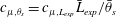
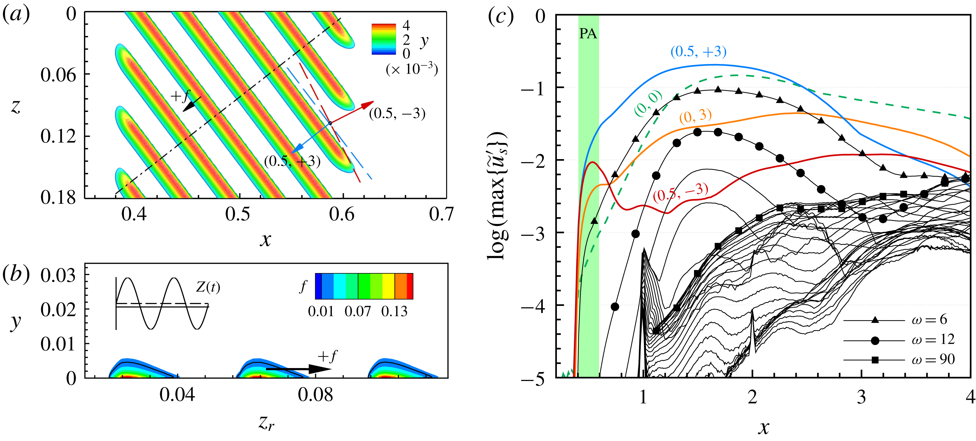
For a successful UFD, the control CF vortices have to be (i) narrowly spaced so that they possibly saturate with lower amplitude without invoking significant secondary instability and (ii) strongly amplified at first so that they can dominate the primary state and generate a beneficial mean-flow distortion. Among the candidates, the narrowly spaced, rightward-travelling CF-vortex modes
 $(0.5,+3)$
and
$(0.5,+3)$
and
 $(1,+3)$
are strongly amplified in the leading-edge region but damped for
$(1,+3)$
are strongly amplified in the leading-edge region but damped for
 $x>2.9$
and
$x>2.9$
and
 $x>2.4$
, respectively. The leftward-travelling modes
$x>2.4$
, respectively. The leftward-travelling modes
 $(0.5,-3)$
and
$(0.5,-3)$
and
 $(1,-3)$
are amplified over a longer distance but their maximal amplification rates are distinctly lower. For an overview of the stability properties of the CF-vortex modes with higher frequencies, the dependence of the spatial amplification rate
$(1,-3)$
are amplified over a longer distance but their maximal amplification rates are distinctly lower. For an overview of the stability properties of the CF-vortex modes with higher frequencies, the dependence of the spatial amplification rate
 $\unicode[STIX]{x1D6FC}_{i}$
on
$\unicode[STIX]{x1D6FC}_{i}$
on
 $\unicode[STIX]{x1D6FE}$
and
$\unicode[STIX]{x1D6FE}$
and
 $\unicode[STIX]{x1D714}$
at two chordwise positions is shown in figure 5. The rightward-travelling modes are generally more unstable. At
$\unicode[STIX]{x1D714}$
at two chordwise positions is shown in figure 5. The rightward-travelling modes are generally more unstable. At
 $x=1.0$
the highest amplification is found for
$x=1.0$
the highest amplification is found for
 $\unicode[STIX]{x1D714}\approx 12$
and
$\unicode[STIX]{x1D714}\approx 12$
and
 $\unicode[STIX]{x1D6FE}\approx 80$
. Farther downstream at
$\unicode[STIX]{x1D6FE}\approx 80$
. Farther downstream at
 $x=2.0$
, the unstable wavenumber range shrinks stronger with increasing frequency. As also proven by preliminary investigations using DNS, the CF-vortex modes with higher frequencies are amplified only in a short region and strongly damped downstream. Hence, the mean-flow distortion generated is not sufficient to effectively stabilize the flow. Further findings of our preliminary investigations of the influence of
$x=2.0$
, the unstable wavenumber range shrinks stronger with increasing frequency. As also proven by preliminary investigations using DNS, the CF-vortex modes with higher frequencies are amplified only in a short region and strongly damped downstream. Hence, the mean-flow distortion generated is not sufficient to effectively stabilize the flow. Further findings of our preliminary investigations of the influence of
 $\unicode[STIX]{x1D6FE}$
and
$\unicode[STIX]{x1D6FE}$
and
 $\unicode[STIX]{x1D714}$
are summarized at the end of § 4.1.
$\unicode[STIX]{x1D714}$
are summarized at the end of § 4.1.
3.2 Reference cases
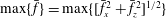
Downstream development of modal
 $\tilde{u} _{s,(h,k)}^{\prime }$
and
$\tilde{u} _{s,(h,k)}^{\prime }$
and
 $\tilde{u} _{s,(h)}^{\prime }$
amplitudes for (a) case REF-S and (b) case REF-U from Fourier analysis (maximum over
$\tilde{u} _{s,(h)}^{\prime }$
amplitudes for (a) case REF-S and (b) case REF-U from Fourier analysis (maximum over
 $y$
or
$y$
or
 $y$
and
$y$
and
 $z$
,
$z$
,
 $6\leqslant \unicode[STIX]{x1D714}\leqslant 180$
,
$6\leqslant \unicode[STIX]{x1D714}\leqslant 180$
,
 $\unicode[STIX]{x0394}\unicode[STIX]{x1D714}=6$
).
$\unicode[STIX]{x0394}\unicode[STIX]{x1D714}=6$
).
Definition of investigated cases.
We provide two reference cases with a single steady or unsteady mode as primary disturbance input, respectively. In both cases the plasma actuators are inactive. Table 2 summarizes the disturbance inputs for the various cases presented in this paper. For case REF-S the most amplified steady mode
 $(0,2)$
is excited by the primary disturbance strip. In figure 6, the modal amplitude development of the streamline-oriented disturbance velocity component
$(0,2)$
is excited by the primary disturbance strip. In figure 6, the modal amplitude development of the streamline-oriented disturbance velocity component
 $\tilde{u} _{s}^{\prime }=u_{s}^{\prime }/u_{B,s,e}=(u_{s}-u_{B,s})/u_{B,s,e}$
is shown. The amplitude of the mode
$\tilde{u} _{s}^{\prime }=u_{s}^{\prime }/u_{B,s,e}=(u_{s}-u_{B,s})/u_{B,s,e}$
is shown. The amplitude of the mode
 $(0,2)$
surpasses
$(0,2)$
surpasses
 $10\,\%$
of
$10\,\%$
of
 $u_{B,s,e}$
at
$u_{B,s,e}$
at
 $x\approx 2.2$
while the amplification rate progressively decreases proceeding further into the saturation state. Convective secondary instability is triggered by the large-amplitude CF vortices for
$x\approx 2.2$
while the amplification rate progressively decreases proceeding further into the saturation state. Convective secondary instability is triggered by the large-amplitude CF vortices for
 $x>2.5$
. The strong secondary growth of the high-frequency mode
$x>2.5$
. The strong secondary growth of the high-frequency mode
 $\unicode[STIX]{x1D714}=90$
is followed by further amplification of higher-frequency unsteady components, leading to the transition to turbulence. Figure 7(a) shows the vortical structures in the rotated reference system
$\unicode[STIX]{x1D714}=90$
is followed by further amplification of higher-frequency unsteady components, leading to the transition to turbulence. Figure 7(a) shows the vortical structures in the rotated reference system
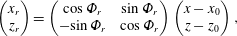 $$\begin{eqnarray}\displaystyle \left(\begin{array}{@{}c@{}}x_{r}\\ z_{r}\end{array}\right)=\left(\begin{array}{@{}cc@{}}\cos \unicode[STIX]{x1D6F7}_{r} & \sin \unicode[STIX]{x1D6F7}_{r}\\ -\sin \,\unicode[STIX]{x1D6F7}_{r} & \cos \unicode[STIX]{x1D6F7}_{r}\end{array}\right)\left(\begin{array}{@{}c@{}}x-x_{0}\\ z-z_{0}\end{array}\right), & & \displaystyle\end{eqnarray}$$
with
 $x_{0}=0.4$
,
$x_{0}=0.4$
,
 $z_{0}=0$
and
$z_{0}=0$
and
 $\unicode[STIX]{x1D6F7}=45^{\circ }$
. In the physical space, steady CF vortices corresponding to the mode
$\unicode[STIX]{x1D6F7}=45^{\circ }$
. In the physical space, steady CF vortices corresponding to the mode
 $(0,2)$
appear, with axes nearly parallel to the potential-flow streamlines. The finger-like high-frequency secondary structures emerge on the main CF vortices and convect downstream, finally developing into turbulence spots.
$(0,2)$
appear, with axes nearly parallel to the potential-flow streamlines. The finger-like high-frequency secondary structures emerge on the main CF vortices and convect downstream, finally developing into turbulence spots.
Vortex visualization (snapshots,
 $\unicode[STIX]{x1D706}_{2}=-4$
, colour indicates
$\unicode[STIX]{x1D706}_{2}=-4$
, colour indicates
 $y$
) for case REF-S at
$y$
) for case REF-S at
 $t/T_{0}=18$
(a) and case REF-U at
$t/T_{0}=18$
(a) and case REF-U at
 $t/T_{0}=17.25$
(b), 17.5 (c), 17.75 (d) and 18 (e). The rotated reference system according to (3.1) is used. Note the compression of the
$t/T_{0}=17.25$
(b), 17.5 (c), 17.75 (d) and 18 (e). The rotated reference system according to (3.1) is used. Note the compression of the
 $x_{r}$
-axis (
$x_{r}$
-axis (
 $z_{r}:x_{r}=2:1$
).
$z_{r}:x_{r}=2:1$
).
In case REF-U the most amplified unsteady mode
 $(1,+2)$
is excited as primary disturbance. The forcing amplitude of the primary disturbance strip is chosen such that the amplitude of the primary mode
$(1,+2)$
is excited as primary disturbance. The forcing amplitude of the primary disturbance strip is chosen such that the amplitude of the primary mode
 $(1,+2)$
reaches the same level at
$(1,+2)$
reaches the same level at
 $x=2.2$
as that of mode
$x=2.2$
as that of mode
 $(0,2)$
in REF-S; see figure 6(b). In accordance with results of linear stability analysis, the amplification of the unsteady mode
$(0,2)$
in REF-S; see figure 6(b). In accordance with results of linear stability analysis, the amplification of the unsteady mode
 $(1,+2)$
is significantly stronger, i.e. only a smaller initial amplitude of the mode
$(1,+2)$
is significantly stronger, i.e. only a smaller initial amplitude of the mode
 $(1,+2)$
is required;
$(1,+2)$
is required;
 $(1,+2)$
saturates earlier than
$(1,+2)$
saturates earlier than
 $(0,2)$
in REF-S and triggers somewhat stronger secondary instability at about the same
$(0,2)$
in REF-S and triggers somewhat stronger secondary instability at about the same
 $x$
-position. The background disturbances rise explosively downstream of their forcing, leading to rapid transition. In figure 7(b–e), snapshots of the vortical structures at four time instances within a fundamental period
$x$
-position. The background disturbances rise explosively downstream of their forcing, leading to rapid transition. In figure 7(b–e), snapshots of the vortical structures at four time instances within a fundamental period
 $T_{0}$
are presented. The CF vortices are travelling in positive spanwise and
$T_{0}$
are presented. The CF vortices are travelling in positive spanwise and
 $x_{r}$
direction. The finger-like structures emerge on the main CF vortices and ride along them.
$x_{r}$
direction. The finger-like structures emerge on the main CF vortices and ride along them.
4 Investigations of control
The inherent unsteady force production of plasma actuators provides good opportunities for exciting narrowly spaced travelling CF-vortex modes as UFD control modes. However, whereas a comprehensive fundamental study of the mechanism of the steady UFD technique has already been conducted by Wassermann & Kloker (Reference Wassermann and Kloker2002), the potential of the narrowly spaced, travelling CF-vortex modes as UFD control modes has not been clarified so far. In § 4.1 we first investigate the modification of the flow field by single travelling CF-vortex modes as UFD modes, excited by blowing/suction, and the resulting stability properties of the two-dimensional mean flow. Secondly, unsteady volume-force actuators are set based on the findings of this fundamental study. The flow deformation by unsteady volume forcing and its ability to delay the transition are discussed in §§ 4.2 and 4.3, respectively.
4.1 Single travelling UFD modes excited by blowing/suction
In cases BS-UFD-R and BS-UFD-L, the actuator row for UFD is set at
 $x=0.5$
by an additional blowing/suction strip extending over
$x=0.5$
by an additional blowing/suction strip extending over
 $0.481\leqslant x\leqslant 0.520$
, exciting the single control mode
$0.481\leqslant x\leqslant 0.520$
, exciting the single control mode
 $(0.5,+3)$
or
$(0.5,+3)$
or
 $(0.5,-3)$
, respectively. The amplitude of the blowing/suction is kept identical for both cases. To clarify the pure effect of the travelling UFD modes, the strip for primary (‘test-mode’) disturbance input at
$(0.5,-3)$
, respectively. The amplitude of the blowing/suction is kept identical for both cases. To clarify the pure effect of the travelling UFD modes, the strip for primary (‘test-mode’) disturbance input at
 $x=0.8$
is deactivated. For indication of secondary instabilities that might possibly arise farther upstream, (background) pulsing at
$x=0.8$
is deactivated. For indication of secondary instabilities that might possibly arise farther upstream, (background) pulsing at
 $x=1.0$
and
$x=1.0$
and
 $x=2.0$
is introduced for both cases.
$x=2.0$
is introduced for both cases.
4.1.1 Development of disturbance amplitudes
Like figure 6 but for (a) case BS-UFD-R and (b) case BS-UFD-L.
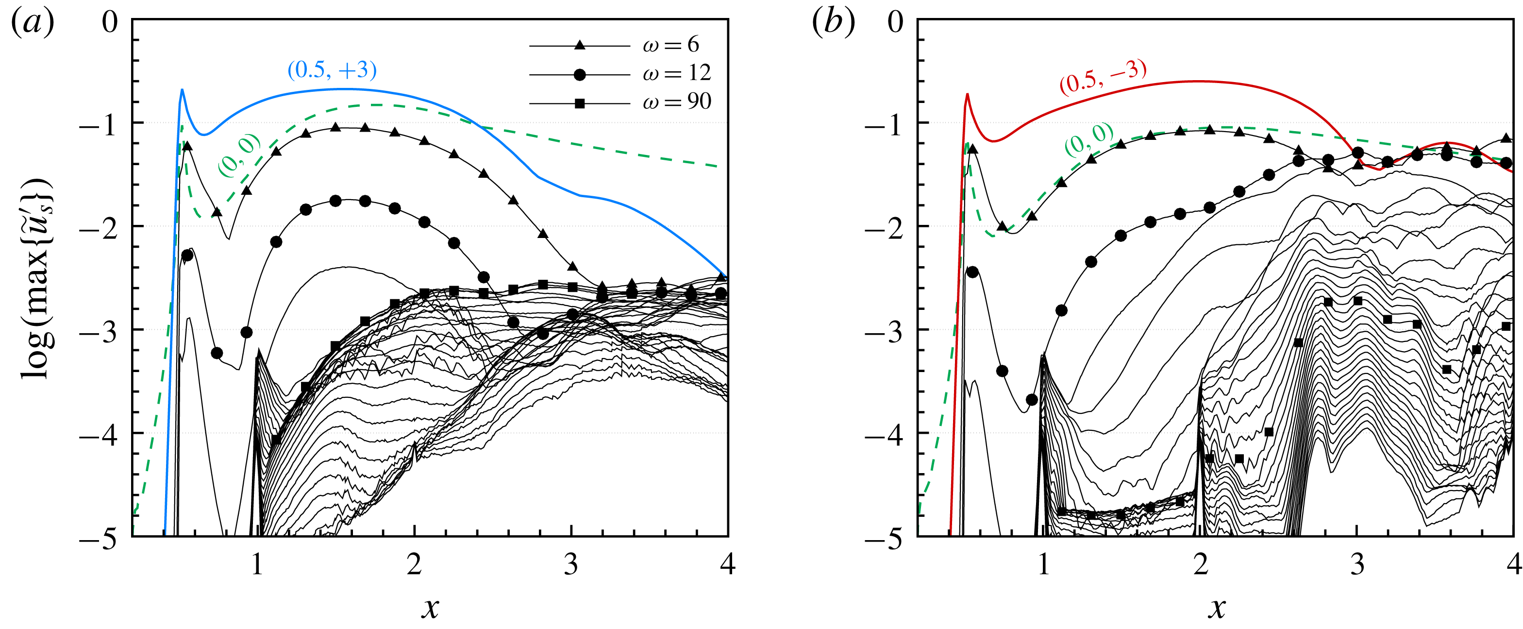
In case BS-UFD-R the rightward-travelling mode
 $(0.5,+3)$
saturates at
$(0.5,+3)$
saturates at
 $x\approx 1.6$
with an amplitude level of 21 %; see figure 8(a). Upstream of the secondary pulsing, the superharmonics of
$x\approx 1.6$
with an amplitude level of 21 %; see figure 8(a). Upstream of the secondary pulsing, the superharmonics of
 $(0.5,+3)$
are represented by the lower-frequency curves resulting from the
$(0.5,+3)$
are represented by the lower-frequency curves resulting from the
 $t$
-modal decomposition. In addition, a strong mean-flow distortion
$t$
-modal decomposition. In addition, a strong mean-flow distortion
 $(0,0)$
is nonlinearly generated. According to linear stability analysis, the mode
$(0,0)$
is nonlinearly generated. According to linear stability analysis, the mode
 $(0.5,+3)$
is damped only downstream of
$(0.5,+3)$
is damped only downstream of
 $x\approx 2.9$
. However, due to the stabilizing effect of the mean-flow distortion
$x\approx 2.9$
. However, due to the stabilizing effect of the mean-flow distortion
 $(0,0)$
as discussed in § 4.1.3, the damping of
$(0,0)$
as discussed in § 4.1.3, the damping of
 $(0.5,+3)$
occurs earlier. It decays monotonically to an amplitude level of 0.3 % at the end of the considered domain, whereas the mean-flow distortion
$(0.5,+3)$
occurs earlier. It decays monotonically to an amplitude level of 0.3 % at the end of the considered domain, whereas the mean-flow distortion
 $(0,0)$
is more persistent. Unlike the reference cases REF-S and REF-U, no strong, persistent secondary instability is triggered. At the end of the domain all unsteady modes fall far below 1 %. In case BS-UFD-L, as shown in figure 8(b), the leftward-travelling mode
$(0,0)$
is more persistent. Unlike the reference cases REF-S and REF-U, no strong, persistent secondary instability is triggered. At the end of the domain all unsteady modes fall far below 1 %. In case BS-UFD-L, as shown in figure 8(b), the leftward-travelling mode
 $(0.5,-3)$
is amplified more weakly than
$(0.5,-3)$
is amplified more weakly than
 $(0.5,+3)$
and attains saturation with an amplitude of 25 % at
$(0.5,+3)$
and attains saturation with an amplitude of 25 % at
 $x\approx 2.0$
, farther downstream than
$x\approx 2.0$
, farther downstream than
 $(0.5,+3)$
. Nevertheless, the maximal amplitude of the nonlinearly generated mean-flow distortion
$(0.5,+3)$
. Nevertheless, the maximal amplitude of the nonlinearly generated mean-flow distortion
 $(0,0)$
is significantly lower than in case BS-UFD-R. Farther downstream, a significant growth of all unsteady disturbance components is observed. Since both the superharmonics of the unsteady primary mode and the secondarily unstable modes may contribute to this growth, secondary instabilities cannot be clearly identified.
$(0,0)$
is significantly lower than in case BS-UFD-R. Farther downstream, a significant growth of all unsteady disturbance components is observed. Since both the superharmonics of the unsteady primary mode and the secondarily unstable modes may contribute to this growth, secondary instabilities cannot be clearly identified.
Downstream development of modal
 $\tilde{u} _{s,m(l)}^{\prime }$
amplitudes in moving systems for (a) case BS-UFD-R and (b) case BS-UFD-L from Fourier analysis (maximum over
$\tilde{u} _{s,m(l)}^{\prime }$
amplitudes in moving systems for (a) case BS-UFD-R and (b) case BS-UFD-L from Fourier analysis (maximum over
 $y$
and
$y$
and
 $z$
,
$z$
,
 $\unicode[STIX]{x1D714}_{m}=0$
and
$\unicode[STIX]{x1D714}_{m}=0$
and
 $5\leqslant \unicode[STIX]{x1D714}_{m}\leqslant 179$
,
$5\leqslant \unicode[STIX]{x1D714}_{m}\leqslant 179$
,
 $\unicode[STIX]{x0394}\unicode[STIX]{x1D714}_{m}=6$
). (c) Illustration of the connection between the (
$\unicode[STIX]{x0394}\unicode[STIX]{x1D714}_{m}=6$
). (c) Illustration of the connection between the (
 $t$
–
$t$
–
 $z$
)-modal decomposition in the fixed system and the
$z$
)-modal decomposition in the fixed system and the
 $t$
-modal decomposition in the Galilean-transformed system moving with the mode
$t$
-modal decomposition in the Galilean-transformed system moving with the mode
 $(0.5,+3)$
(left) and
$(0.5,+3)$
(left) and
 $(0.5,-3)$
(right), respectively. The frequency factor in the moving system is denoted by
$(0.5,-3)$
(right), respectively. The frequency factor in the moving system is denoted by
 $l$
instead of
$l$
instead of
 $h$
with
$h$
with
 $\unicode[STIX]{x1D714}_{m}=l\unicode[STIX]{x1D714}_{0}$
.
$\unicode[STIX]{x1D714}_{m}=l\unicode[STIX]{x1D714}_{0}$
.
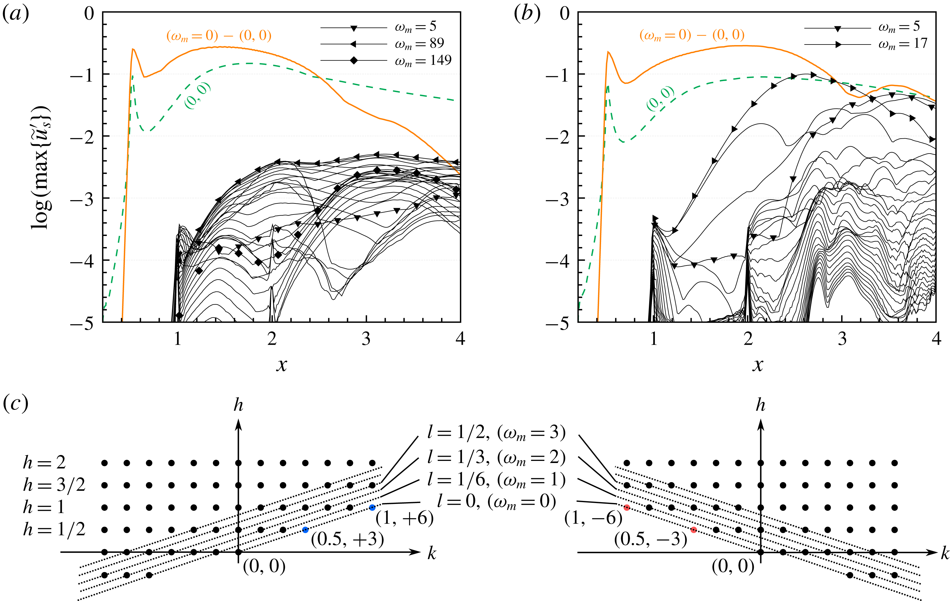
In order to unambiguously clarify the secondary instabilities triggered, we analyse the amplitude development referring to a Galilean-transformed system
 $(x,y,z_{m})$
, see Wassermann & Kloker (Reference Wassermann and Kloker2003),
$(x,y,z_{m})$
, see Wassermann & Kloker (Reference Wassermann and Kloker2003),
 $z_{m}=z-c_{(0.5,\pm 3)}t$
, where
$z_{m}=z-c_{(0.5,\pm 3)}t$
, where
 $c_{(0.5,\pm 3)}=\pm 0.5\unicode[STIX]{x1D714}_{0}/(3\unicode[STIX]{x1D6FE}_{0})$
is the spanwise phase velocity of the primary mode
$c_{(0.5,\pm 3)}=\pm 0.5\unicode[STIX]{x1D714}_{0}/(3\unicode[STIX]{x1D6FE}_{0})$
is the spanwise phase velocity of the primary mode
 $(0.5,\pm 3)$
. With respect to the transformed moving system, the primary state becomes steady. The modal component
$(0.5,\pm 3)$
. With respect to the transformed moving system, the primary state becomes steady. The modal component
 $\unicode[STIX]{x1D714}_{m}=0$
consists of a spanwise mean
$\unicode[STIX]{x1D714}_{m}=0$
consists of a spanwise mean
 $(0,0)$
and a purely three-dimensional component
$(0,0)$
and a purely three-dimensional component
 $(\unicode[STIX]{x1D714}_{m}=0)-(0,0)$
that can be recomposed by the primary mode and its superharmonics; see figure 9(c). Furthermore, other (
$(\unicode[STIX]{x1D714}_{m}=0)-(0,0)$
that can be recomposed by the primary mode and its superharmonics; see figure 9(c). Furthermore, other (
 $t$
–
$t$
–
 $z$
)-modal components belonging to the same secondary instability mode carried by the primary wave, i.e. on the same diagonal as sketched in figure 9(c), are recombined. The secondary-instability behaviour is directly indicated by the modal components
$z$
)-modal components belonging to the same secondary instability mode carried by the primary wave, i.e. on the same diagonal as sketched in figure 9(c), are recombined. The secondary-instability behaviour is directly indicated by the modal components
 $\unicode[STIX]{x1D714}_{m}\neq 0$
.
$\unicode[STIX]{x1D714}_{m}\neq 0$
.
For case BS-UFD-R (figure 9
a), secondary instabilities are observed in a short region downstream of the pulsing at
 $x=1.0$
. The leading mode
$x=1.0$
. The leading mode
 $\unicode[STIX]{x1D714}_{m}=89$
reaches an amplitude of 0.4 % at
$\unicode[STIX]{x1D714}_{m}=89$
reaches an amplitude of 0.4 % at
 $x=2.1$
and becomes virtually stable farther downstream. For
$x=2.1$
and becomes virtually stable farther downstream. For
 $2.0<x<3.0$
a distinct secondary growth is found for the modes with higher frequencies. At the end of the domain, the three-dimensional flow deformation dies out, and almost all unsteady components are stable. Within the considered domain, none of the secondary instability modes exceeds an amplitude of 0.5 %. For case BS-UFD-L (figure 9
b), some low-frequency modes undergo a strong amplification. Farther downstream, the leading mode with
$2.0<x<3.0$
a distinct secondary growth is found for the modes with higher frequencies. At the end of the domain, the three-dimensional flow deformation dies out, and almost all unsteady components are stable. Within the considered domain, none of the secondary instability modes exceeds an amplitude of 0.5 %. For case BS-UFD-L (figure 9
b), some low-frequency modes undergo a strong amplification. Farther downstream, the leading mode with
 $\unicode[STIX]{x1D714}_{m}=17$
becomes nonlinear, significantly alters the primary state downstream and possibly drives the filling up of the perturbation spectrum. Compared to the rightward-travelling UFD mode
$\unicode[STIX]{x1D714}_{m}=17$
becomes nonlinear, significantly alters the primary state downstream and possibly drives the filling up of the perturbation spectrum. Compared to the rightward-travelling UFD mode
 $(0.5,+3)$
or the steady mode
$(0.5,+3)$
or the steady mode
 $(0,3)$
, the mode
$(0,3)$
, the mode
 $(0.5,-3)$
seems more susceptible to low-frequency secondary instability.
$(0.5,-3)$
seems more susceptible to low-frequency secondary instability.
When examining the normalized modal
 $u_{r}^{\prime }$
amplitude distribution in crosscuts in the rotated moving system
$u_{r}^{\prime }$
amplitude distribution in crosscuts in the rotated moving system
 $$\begin{eqnarray}\displaystyle \left(\begin{array}{@{}c@{}}x_{r,m}\\ z_{r,m}\end{array}\right)=\left(\begin{array}{@{}cc@{}}\cos \unicode[STIX]{x1D6F7}_{r} & \sin \unicode[STIX]{x1D6F7}_{r}\\ -\sin \,\unicode[STIX]{x1D6F7}_{r} & \cos \unicode[STIX]{x1D6F7}_{r}\end{array}\right)\left(\begin{array}{@{}c@{}}x-x_{0}\\ z-c_{(0.5,\pm 3)}t-z_{0}\end{array}\right), & & \displaystyle\end{eqnarray}$$
with
 $x_{0}=0.4$
,
$x_{0}=0.4$
,
 $z_{0}=0$
and
$z_{0}=0$
and
 $\unicode[STIX]{x1D6F7}=45^{\circ }$
, the origin of the secondary instabilities becomes transparent. For case BS-UFD-R at
$\unicode[STIX]{x1D6F7}=45^{\circ }$
, the origin of the secondary instabilities becomes transparent. For case BS-UFD-R at
 $x_{r,m}=1.5$
(
$x_{r,m}=1.5$
(
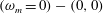
 $x\approx 1.4$
), as shown in figure 10(a), a type-I or
$x\approx 1.4$
), as shown in figure 10(a), a type-I or
 $z$
-mode is found for
$z$
-mode is found for
 $\unicode[STIX]{x1D714}_{m}=89$
which attains the largest amplitude. Farther downstream, this mode spreads upwards to the top region of the shear layer, likely reflecting both
$\unicode[STIX]{x1D714}_{m}=89$
which attains the largest amplitude. Farther downstream, this mode spreads upwards to the top region of the shear layer, likely reflecting both
 $z$
- and
$z$
- and
 $y$
-modes; see crosscut at
$y$
-modes; see crosscut at
 $x_{r,m}=3.0$
(
$x_{r,m}=3.0$
(
 $x\approx 2.5$
) in figure 10(b). The high-frequency component
$x\approx 2.5$
) in figure 10(b). The high-frequency component
 $\unicode[STIX]{x1D714}_{m}=149$
, being one of the most amplified secondary instability modes at this position, reveals a typical amplitude distribution of a type-II or
$\unicode[STIX]{x1D714}_{m}=149$
, being one of the most amplified secondary instability modes at this position, reveals a typical amplitude distribution of a type-II or
 $y$
-mode; see figure 10(d). Once the three-dimensional deformation fades out, the originally localized secondary modes are gradually smeared; see figure 10(c,e). In case BS-UFD-L, the mode
$y$
-mode; see figure 10(d). Once the three-dimensional deformation fades out, the originally localized secondary modes are gradually smeared; see figure 10(c,e). In case BS-UFD-L, the mode
 $\unicode[STIX]{x1D714}_{m}=17$
is a typical type-III mode which is located in the near-wall region at the updraft side of the main CF vortices (figure 10
f,g). At
$\unicode[STIX]{x1D714}_{m}=17$
is a typical type-III mode which is located in the near-wall region at the updraft side of the main CF vortices (figure 10
f,g). At
 $x_{r,m}=3.0$
, the vortical structures in the near-wall region are strongly modified, leading to an increase of the complexity of the shear layers.
$x_{r,m}=3.0$
, the vortical structures in the near-wall region are strongly modified, leading to an increase of the complexity of the shear layers.
Crosscuts for (a–e) case BS-UFD-R and (f,g) case BS-UFD-L at various downstream positions in the rotated reference system moving spanwise with the respective primary CF vortices. Dashed lines:
 $\unicode[STIX]{x1D706}_{2}$
isocontours (
$\unicode[STIX]{x1D706}_{2}$
isocontours (
 $-12$
to
$-12$
to
 $-2$
,
$-2$
,
 $\unicode[STIX]{x1D6E5}=2$
); solid lines:
$\unicode[STIX]{x1D6E5}=2$
); solid lines:
 $\tilde{u} _{r}$
isocontours (0.05 to 0.95,
$\tilde{u} _{r}$
isocontours (0.05 to 0.95,
 $\unicode[STIX]{x1D6E5}=0.10$
); colour: normalized modal
$\unicode[STIX]{x1D6E5}=0.10$
); colour: normalized modal
 $u_{r}^{\prime }$
amplitude distribution.
$u_{r}^{\prime }$
amplitude distribution.
4.1.2 Vortical structures
Vortex visualization (snapshots,
 $\unicode[STIX]{x1D706}_{2}=-2.5$
, colour indicates
$\unicode[STIX]{x1D706}_{2}=-2.5$
, colour indicates
 $y$
) for (a) case BS-UFD-R and (b) case BS-UFD-L at
$y$
) for (a) case BS-UFD-R and (b) case BS-UFD-L at
 $t/T_{0}=18$
. Rotated (fixed) reference system according to (3.1) is used. Note the compression of the
$t/T_{0}=18$
. Rotated (fixed) reference system according to (3.1) is used. Note the compression of the
 $x_{r}$
-axis (
$x_{r}$
-axis (
 $z_{r}:x_{r}=2:1$
). Arrows indicate the travelling directions of the CF vortices.
$z_{r}:x_{r}=2:1$
). Arrows indicate the travelling directions of the CF vortices.

The snapshots of the vortical structures arising in cases BS-UFD-R and BS-UFD-L are shown in figures 11(a) and 11(b), respectively. In both cases, the main CF vortices triggered by blowing and suction are spaced more narrowly than those arising in cases REF-S and REF-U. We note the misalignment between the orientation of the main vortices in both cases. In accordance with the modal amplitude development, the primary CF vortices in case BS-UFD-R die out downstream of
 $x_{r}=3.9$
(
$x_{r}=3.9$
(
 $x\approx 3.1$
). The finger-like secondary structures, left over from the high-frequency type-I and type-II modes upstream, are distorted, and stretched in the spanwise direction. Unlike the turbulent spots appearing in the reference cases, these structures are situated farther away from the wall and cause no skin-friction increase (not shown). In case BS-UFD-L, the main CF vortices are visible up to
$x\approx 3.1$
). The finger-like secondary structures, left over from the high-frequency type-I and type-II modes upstream, are distorted, and stretched in the spanwise direction. Unlike the turbulent spots appearing in the reference cases, these structures are situated farther away from the wall and cause no skin-friction increase (not shown). In case BS-UFD-L, the main CF vortices are visible up to
 $x_{r}=4.5$
(
$x_{r}=4.5$
(
 $x\approx 3.5$
). Each main CF vortex is accompanied by a counter-rotating CF vortex at the updraft side, which is strongly modulated by the secondarily amplified modes downstream of the pulsing. Since the secondary structures are mainly evolved from the low-frequency type-III mode
$x\approx 3.5$
). Each main CF vortex is accompanied by a counter-rotating CF vortex at the updraft side, which is strongly modulated by the secondarily amplified modes downstream of the pulsing. Since the secondary structures are mainly evolved from the low-frequency type-III mode
 $\unicode[STIX]{x1D714}_{m}=17$
, their shapes are significantly different from the finger-like structures arising on the top side of the main CF vortices in case BS-UFD-R. See Bonfigli & Kloker (Reference Bonfigli and Kloker2007) for a detailed comparison between the vortical structures resulting from different secondary instability modes.
$\unicode[STIX]{x1D714}_{m}=17$
, their shapes are significantly different from the finger-like structures arising on the top side of the main CF vortices in case BS-UFD-R. See Bonfigli & Kloker (Reference Bonfigli and Kloker2007) for a detailed comparison between the vortical structures resulting from different secondary instability modes.
4.1.3 Modification of mean-flow profiles and stability properties
For the classical UFD technique using a steady control mode it was demonstrated that the growth attenuation of the primary modes is mainly based on the mean-flow distortion
 $(0,0)$
, which has a stabilizing effect similar to homogeneous suction; see Wassermann & Kloker (Reference Wassermann and Kloker2002). In order to verify whether the
$(0,0)$
, which has a stabilizing effect similar to homogeneous suction; see Wassermann & Kloker (Reference Wassermann and Kloker2002). In order to verify whether the
 $(0,0)$
generated by unsteady control modes also has the same stabilizing effect, the streamwise and crosswise velocity profiles are averaged in time and spanwise direction, and then analysed in terms of the stability properties using linear stability calculations. Since case BS-UFD-L shows transition to turbulence it is ruled out and in the following we concentrate on case BS-UFD-R.
$(0,0)$
generated by unsteady control modes also has the same stabilizing effect, the streamwise and crosswise velocity profiles are averaged in time and spanwise direction, and then analysed in terms of the stability properties using linear stability calculations. Since case BS-UFD-L shows transition to turbulence it is ruled out and in the following we concentrate on case BS-UFD-R.
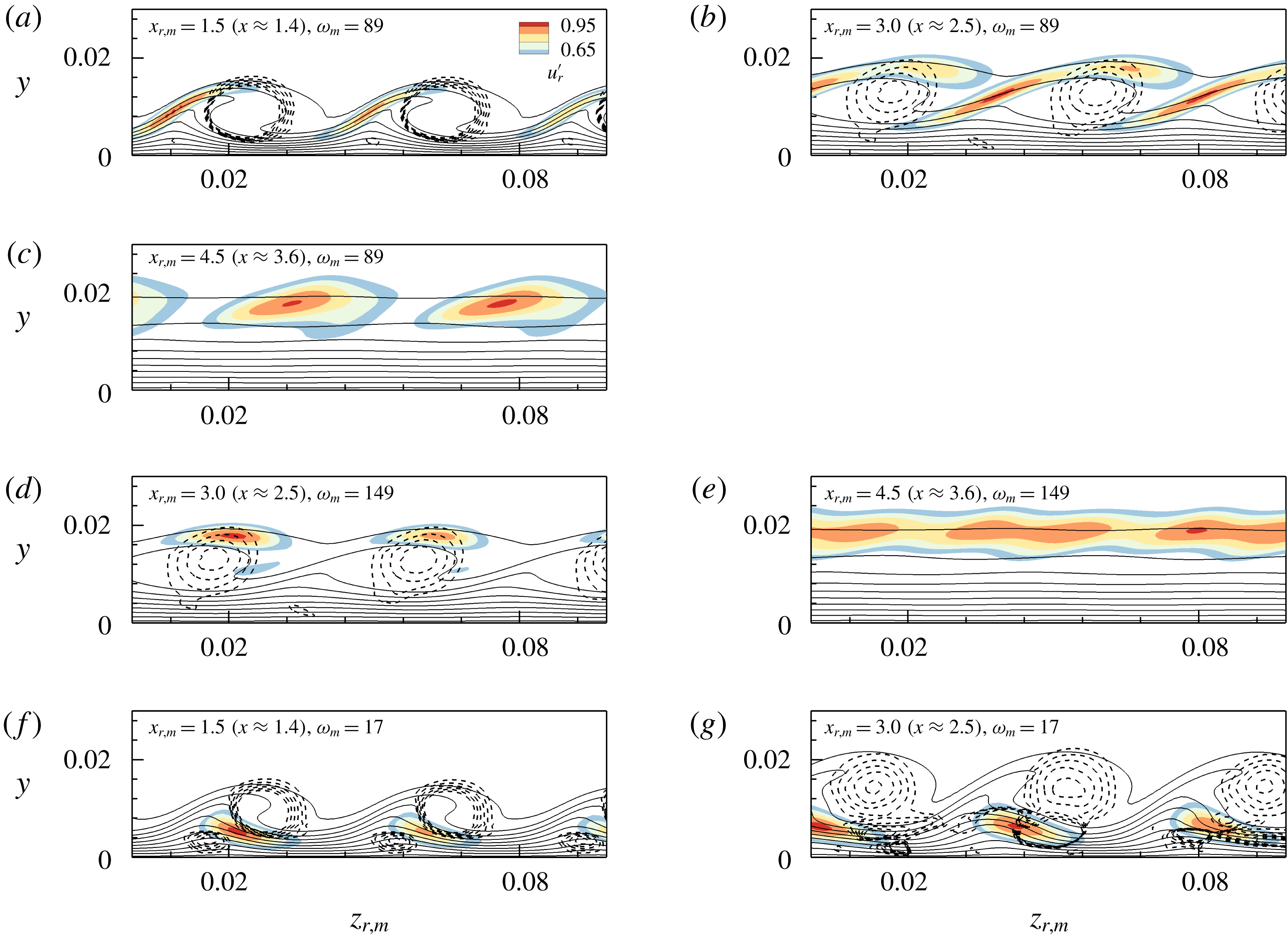
Time- and spanwise-averaged (a)
 $\tilde{u} _{s,tzm}$
and (b)
$\tilde{u} _{s,tzm}$
and (b)
 $\tilde{w}_{s,tzm}$
profiles for case BS-UFD-R in comparison to the corresponding base flow at various downstream positions (
$\tilde{w}_{s,tzm}$
profiles for case BS-UFD-R in comparison to the corresponding base flow at various downstream positions (
 $x=0.8$
, 1.2, 1.8, 2.4, 3.0, 3.6 from left to right; the abscissa shift is 0.5 and 0.1, respectively).
$x=0.8$
, 1.2, 1.8, 2.4, 3.0, 3.6 from left to right; the abscissa shift is 0.5 and 0.1, respectively).
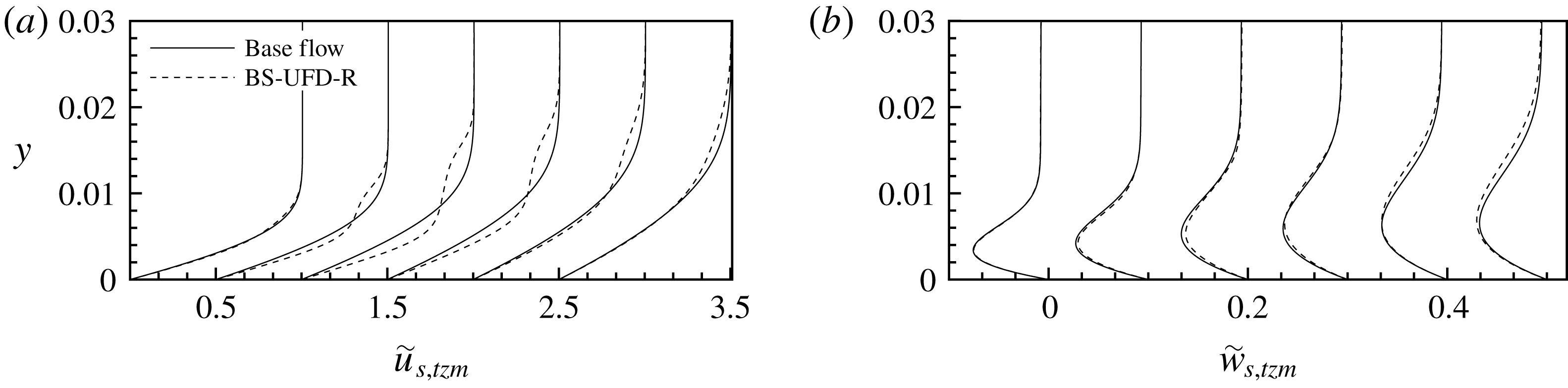
Figure 12 shows that the
 $\tilde{u} _{s,tzm}$
profiles are S-shaped with increase in the near-wall region and decrease farther away from the wall. The CF component
$\tilde{u} _{s,tzm}$
profiles are S-shaped with increase in the near-wall region and decrease farther away from the wall. The CF component
 $\tilde{w}_{s,tzm}$
is only slightly reduced at
$\tilde{w}_{s,tzm}$
is only slightly reduced at
 $x=1.2$
and 1.8, and even increased farther downstream, questioning a palpable stabilizing effect.
$x=1.2$
and 1.8, and even increased farther downstream, questioning a palpable stabilizing effect.
Spatial chordwise amplification rates
 $\unicode[STIX]{x1D6FC}_{i}$
of unstable CF-vortex modes for case BS-UFD-R in comparison to the corresponding base-flow data (lines with levels 0.0 to
$\unicode[STIX]{x1D6FC}_{i}$
of unstable CF-vortex modes for case BS-UFD-R in comparison to the corresponding base-flow data (lines with levels 0.0 to
 $-4.2$
,
$-4.2$
,
 $\unicode[STIX]{x1D6E5}=0.3$
). (a) Steady modes; the dashed lines mark the modes
$\unicode[STIX]{x1D6E5}=0.3$
). (a) Steady modes; the dashed lines mark the modes
 $(0,2)$
(lower) and
$(0,2)$
(lower) and
 $(0,3)$
(upper). (b) Unsteady modes with
$(0,3)$
(upper). (b) Unsteady modes with
 $\unicode[STIX]{x1D714}=6$
; the dashed lines mark the modes
$\unicode[STIX]{x1D714}=6$
; the dashed lines mark the modes
 $(1,+2)$
(lower) and
$(1,+2)$
(lower) and
 $(1,+3)$
(upper).
$(1,+3)$
(upper).

(a) Wall-normal gradient of
 $\tilde{w}_{s,tzm}$
for case BS-UFD-R in comparison to the corresponding base flow at various downstream positions (
$\tilde{w}_{s,tzm}$
for case BS-UFD-R in comparison to the corresponding base flow at various downstream positions (
 $x=0.8$
, 1.2, 1.8, 2.4, 3.0, 3.6 from left to right; the abscissa shift is 20). (b) Deformation of the velocity profile
$x=0.8$
, 1.2, 1.8, 2.4, 3.0, 3.6 from left to right; the abscissa shift is 20). (b) Deformation of the velocity profile
 $\tilde{w}_{eff,tzm}$
in the wave-vector direction of the travelling mode
$\tilde{w}_{eff,tzm}$
in the wave-vector direction of the travelling mode
 $(1,+2)$
at
$(1,+2)$
at
 $x=2.4$
and (c) the corresponding wall-normal gradients. Here
$x=2.4$
and (c) the corresponding wall-normal gradients. Here
 $\tilde{w}_{eff,tzm}=\tilde{w}_{s,tzm}\cos \unicode[STIX]{x1D719}_{s}+\tilde{u} _{s,tzm}\sin \unicode[STIX]{x1D719}_{s}$
, where
$\tilde{w}_{eff,tzm}=\tilde{w}_{s,tzm}\cos \unicode[STIX]{x1D719}_{s}+\tilde{u} _{s,tzm}\sin \unicode[STIX]{x1D719}_{s}$
, where
 $\unicode[STIX]{x1D719}_{s}$
is the angle between the wave vector and the
$\unicode[STIX]{x1D719}_{s}$
is the angle between the wave vector and the
 $z_{s}$
-direction.
$z_{s}$
-direction.
In figure 13, the stability diagrams for case BS-UFD-R are shown based on the time-averaged flow and one-dimensional eigenfunction linear stability theory. Because the wave vectors of the steady modes are nearly aligned with the
 $z_{s}$
-direction, the
$z_{s}$
-direction, the
 $\tilde{w}_{s,tzm}$
profile plays a decisive role for the instability. In both Wassermann & Kloker (Reference Wassermann and Kloker2002) and Dörr & Kloker (Reference Dörr and Kloker2017), the stabilizing effect of the mean-flow distortion for steady modes was explained as a consequence of the mean CF reduction. In fact, the possible reduction of the maximum wall-normal gradient
$\tilde{w}_{s,tzm}$
profile plays a decisive role for the instability. In both Wassermann & Kloker (Reference Wassermann and Kloker2002) and Dörr & Kloker (Reference Dörr and Kloker2017), the stabilizing effect of the mean-flow distortion for steady modes was explained as a consequence of the mean CF reduction. In fact, the possible reduction of the maximum wall-normal gradient
 $\text{d}\tilde{w}_{s,tzm}/\text{d}y$
at the inflection point is a cause for the attenuation of the inviscid instability. In figure 14(a) the wall-normal gradients
$\text{d}\tilde{w}_{s,tzm}/\text{d}y$
at the inflection point is a cause for the attenuation of the inviscid instability. In figure 14(a) the wall-normal gradients
 $\text{d}\tilde{w}_{s,tzm}/\text{d}y$
are shown at various
$\text{d}\tilde{w}_{s,tzm}/\text{d}y$
are shown at various
 $x$
-positions.
$x$
-positions.
The amplification of the unsteady modes with
 $\unicode[STIX]{x1D714}=6$
is more strongly reduced than that of the steady modes. As the wave vectors of the unsteady modes are misaligned with the
$\unicode[STIX]{x1D714}=6$
is more strongly reduced than that of the steady modes. As the wave vectors of the unsteady modes are misaligned with the
 $z_{s}$
-direction, the
$z_{s}$
-direction, the
 $\tilde{u} _{s,tzm}$
profile comes into play. As shown by Gregory, Stuart & Walker (Reference Gregory, Stuart and Walker1955), the stability properties of three-dimensional modes with a known wave-vector orientation are linked to the velocity profile
$\tilde{u} _{s,tzm}$
profile comes into play. As shown by Gregory, Stuart & Walker (Reference Gregory, Stuart and Walker1955), the stability properties of three-dimensional modes with a known wave-vector orientation are linked to the velocity profile
 $\tilde{w}_{eff,tzm}=\tilde{w}_{s,tzm}\cos \unicode[STIX]{x1D719}_{s}+\tilde{u} _{s,tzm}\sin \unicode[STIX]{x1D719}_{s}$
, where
$\tilde{w}_{eff,tzm}=\tilde{w}_{s,tzm}\cos \unicode[STIX]{x1D719}_{s}+\tilde{u} _{s,tzm}\sin \unicode[STIX]{x1D719}_{s}$
, where
 $\unicode[STIX]{x1D719}_{s}$
is the angle between the wave vector and the
$\unicode[STIX]{x1D719}_{s}$
is the angle between the wave vector and the
 $z_{s}$
-direction. In figure 14(b,c) the deformation of the velocity profile
$z_{s}$
-direction. In figure 14(b,c) the deformation of the velocity profile
 $\tilde{w}_{eff,tzm}$
regarding the mode
$\tilde{w}_{eff,tzm}$
regarding the mode
 $(1,+2)$
at
$(1,+2)$
at
 $x=2.4$
and the corresponding wall-normal gradients are illustrated. Due to the S-formed
$x=2.4$
and the corresponding wall-normal gradients are illustrated. Due to the S-formed
 $\tilde{u} _{s,tzm}$
profiles, the maximal gradient of
$\tilde{u} _{s,tzm}$
profiles, the maximal gradient of
 $\tilde{w}_{eff,tzm}$
is strongly reduced and the inflection point is shifted distinctly closer to the wall. Hence, the unsteady mode
$\tilde{w}_{eff,tzm}$
is strongly reduced and the inflection point is shifted distinctly closer to the wall. Hence, the unsteady mode
 $(1,+2)$
is greatly stabilized.
$(1,+2)$
is greatly stabilized.
Note that based on the inflection point at the upper part of the
 $\tilde{u} _{s,tzm}$
profiles arising from the UFD, a strong amplification of streamwise-travelling Tollmien–Schlichting waves is predicted by one-dimensional linear stability theory. However, they cannot be observed in DNS results because their receptivity and growth are possibly significantly attenuated due to the additional spanwise modulation by the UFD control mode.
$\tilde{u} _{s,tzm}$
profiles arising from the UFD, a strong amplification of streamwise-travelling Tollmien–Schlichting waves is predicted by one-dimensional linear stability theory. However, they cannot be observed in DNS results because their receptivity and growth are possibly significantly attenuated due to the additional spanwise modulation by the UFD control mode.
In addition, various simulations were performed to examine the influence of the frequency and the spanwise wavenumber of the UFD control mode. If the angular frequency
 $\unicode[STIX]{x1D714}$
is increased from 3 to 6 or 9, both the leftward- and rightward-travelling modes propagate faster in the spanwise direction. The shear layers induced inside the boundary layer are more pronounced and the background disturbances are more strongly amplified, counteracting the stabilizing effect of
$\unicode[STIX]{x1D714}$
is increased from 3 to 6 or 9, both the leftward- and rightward-travelling modes propagate faster in the spanwise direction. The shear layers induced inside the boundary layer are more pronounced and the background disturbances are more strongly amplified, counteracting the stabilizing effect of
 $(0,0)$
. The unwanted secondary amplification can be reduced by increasing the spanwise wavenumber of the UFD mode. However, the CF vortices are then spaced closer so that they hinder the vortical motion of each other and decay earlier. As a result, the nonlinearly generated mean-flow distortion with frequency higher than
$(0,0)$
. The unwanted secondary amplification can be reduced by increasing the spanwise wavenumber of the UFD mode. However, the CF vortices are then spaced closer so that they hinder the vortical motion of each other and decay earlier. As a result, the nonlinearly generated mean-flow distortion with frequency higher than
 $\unicode[STIX]{x1D714}=3$
is too weak to stabilize the flow effectively.
$\unicode[STIX]{x1D714}=3$
is too weak to stabilize the flow effectively.
4.2 Excitation of travelling UFD modes by unsteady volume forcing
(a) Plasma-actuator volume-force distribution for case PA-UFD (
 $f_{10\,\%}$
isosurfaces at the time of the maximal forcing, where
$f_{10\,\%}$
isosurfaces at the time of the maximal forcing, where
 $f_{10\,\%}=\max \{(f_{x}^{2}+f_{z}^{2})^{1/2}\}/10=0.017$
; the colour indicates the wall-normal distance
$f_{10\,\%}=\max \{(f_{x}^{2}+f_{z}^{2})^{1/2}\}/10=0.017$
; the colour indicates the wall-normal distance
 $y$
). The dashed lines show the local orientation of the wave fronts of the CF-vortex modes
$y$
). The dashed lines show the local orientation of the wave fronts of the CF-vortex modes
 $(0.5,+3)$
(blue) and
$(0.5,+3)$
(blue) and
 $(0.5,-3)$
(red). (b) Crosscut along the dash-dotted line perpendicular to the electrode axes shown in (a). The colour indicates
$(0.5,-3)$
(red). (b) Crosscut along the dash-dotted line perpendicular to the electrode axes shown in (a). The colour indicates
 $f$
and the solid lines mark the
$f$
and the solid lines mark the
 $f_{10\,\%}$
isosurfaces at the time of the maximal forcing. The inset shows the physical time signal within a fundamental period. (c) Downstream development of modal
$f_{10\,\%}$
isosurfaces at the time of the maximal forcing. The inset shows the physical time signal within a fundamental period. (c) Downstream development of modal
 $\tilde{u} _{s,(h,k)}^{\prime }$
and
$\tilde{u} _{s,(h,k)}^{\prime }$
and
 $\tilde{u} _{s,(h)}^{\prime }$
amplitudes from Fourier analysis (maximum over
$\tilde{u} _{s,(h)}^{\prime }$
amplitudes from Fourier analysis (maximum over
 $y$
or
$y$
or
 $y$
and
$y$
and
 $z$
,
$z$
,
 $6\leqslant \unicode[STIX]{x1D714}\leqslant 180$
,
$6\leqslant \unicode[STIX]{x1D714}\leqslant 180$
,
 $\unicode[STIX]{x0394}\unicode[STIX]{x1D714}=6$
) for case PA-UFD. The green rectangle indicates the chordwise position of the volume forcing.
$\unicode[STIX]{x0394}\unicode[STIX]{x1D714}=6$
) for case PA-UFD. The green rectangle indicates the chordwise position of the volume forcing.
Based on the results in § 4.1, the travelling mode
 $(0.5,+3)$
is chosen as UFD control mode since it causes no impeding secondary growth by itself. In the following, three actuators per fundamental wavelength are located at
$(0.5,+3)$
is chosen as UFD control mode since it causes no impeding secondary growth by itself. In the following, three actuators per fundamental wavelength are located at
 $x=0.5$
, instead of the blowing/suction strip for UFD as used in the former cases. For an optimal excitation of the unsteady UFD mode, the most effective spatial distribution of the volume force used by Dörr & Kloker (Reference Dörr and Kloker2017) for exciting steady CF-vortex modes is followed. The force extends in the wall-normal direction nearly up to the boundary-layer edge. The sinusoidal time signal
$x=0.5$
, instead of the blowing/suction strip for UFD as used in the former cases. For an optimal excitation of the unsteady UFD mode, the most effective spatial distribution of the volume force used by Dörr & Kloker (Reference Dörr and Kloker2017) for exciting steady CF-vortex modes is followed. The force extends in the wall-normal direction nearly up to the boundary-layer edge. The sinusoidal time signal
 $Z(t)=0.04+0.3\sin (3t)$
is used, i.e. the steady volume force is modulated. Figure 15(a,b) shows the volume-force configuration in top view and in a crosscut. Analogous to the steady forcing, the steady mean of the volume force
$Z(t)=0.04+0.3\sin (3t)$
is used, i.e. the steady volume force is modulated. Figure 15(a,b) shows the volume-force configuration in top view and in a crosscut. Analogous to the steady forcing, the steady mean of the volume force
 $c_{s}f(x,y,z)$
excites steady CF-vortex modes. Meanwhile, the unsteady component
$c_{s}f(x,y,z)$
excites steady CF-vortex modes. Meanwhile, the unsteady component
 $c_{u}f(x,y,z)\sin (\unicode[STIX]{x1D714}_{PA}t)$
imparts an oscillatory perturbation (push and pull events), which excites pairs of leftward- and rightward-travelling waves with the same spanwise wavenumber. Here, using a row of three actuators per fundamental wavelength, operated with angular frequency
$c_{u}f(x,y,z)\sin (\unicode[STIX]{x1D714}_{PA}t)$
imparts an oscillatory perturbation (push and pull events), which excites pairs of leftward- and rightward-travelling waves with the same spanwise wavenumber. Here, using a row of three actuators per fundamental wavelength, operated with angular frequency
 $\unicode[STIX]{x1D714}_{PA}=3$
, a pair of travelling CF-vortex modes
$\unicode[STIX]{x1D714}_{PA}=3$
, a pair of travelling CF-vortex modes
 $(0.5,\pm 3)$
and a weak steady mode
$(0.5,\pm 3)$
and a weak steady mode
 $(0,3)$
are simultaneously excited. Furthermore, the orientation of the electrode axes of the plasma actuators has a significant effect on the receptivity of each individual CF-vortex mode; see also Dörr & Kloker (Reference Dörr and Kloker2017), case CMF. Employing actuators with sufficient length and aligned with the wave front of the desired control mode, the initial amplitude of the corresponding mode can be maximized and the formation of other misaligned modes can be hindered by destructive interference. Therefore, the angle of the actuators,
$(0,3)$
are simultaneously excited. Furthermore, the orientation of the electrode axes of the plasma actuators has a significant effect on the receptivity of each individual CF-vortex mode; see also Dörr & Kloker (Reference Dörr and Kloker2017), case CMF. Employing actuators with sufficient length and aligned with the wave front of the desired control mode, the initial amplitude of the corresponding mode can be maximized and the formation of other misaligned modes can be hindered by destructive interference. Therefore, the angle of the actuators,
 $\unicode[STIX]{x1D6FD}_{PA}$
, is adapted such that the electrode axis is aligned with the axes of the travelling CF vortices arising in case BS-UFD-R at
$\unicode[STIX]{x1D6FD}_{PA}$
, is adapted such that the electrode axis is aligned with the axes of the travelling CF vortices arising in case BS-UFD-R at
 $x=0.5$
to ensure the best receptivity. For the most important actuator parameters, see table 1. The actuators are equidistantly distributed in
$x=0.5$
to ensure the best receptivity. For the most important actuator parameters, see table 1. The actuators are equidistantly distributed in
 $z$
with identical volume-force set-up. The maximal momentum coefficient
$z$
with identical volume-force set-up. The maximal momentum coefficient
 $c_{\unicode[STIX]{x1D707},\unicode[STIX]{x1D703}_{s}}$
based on the momentum thickness
$c_{\unicode[STIX]{x1D707},\unicode[STIX]{x1D703}_{s}}$
based on the momentum thickness
 $\unicode[STIX]{x1D703}_{s}$
at
$\unicode[STIX]{x1D703}_{s}$
at
 $x=0.5$
is
$x=0.5$
is
 $3.5\times 10^{-3}$
, corresponding to 34 % of the most efficient case ACF in Dörr & Kloker (Reference Dörr and Kloker2017). The time-averaged volume force required for the unsteady UFD configuration is reduced to 4 % with respect to case ACF.
$3.5\times 10^{-3}$
, corresponding to 34 % of the most efficient case ACF in Dörr & Kloker (Reference Dörr and Kloker2017). The time-averaged volume force required for the unsteady UFD configuration is reduced to 4 % with respect to case ACF.
To analyse the pure effect of the unsteady volume forcing, the primary disturbance strip at
 $x=0.8$
is inactive for case PA-UFD. Two secondary disturbance strips at
$x=0.8$
is inactive for case PA-UFD. Two secondary disturbance strips at
 $x=1.0$
and
$x=1.0$
and
 $x=2.0$
are used to introduce unsteady (background) disturbances. The modal amplitude development is shown in figure 15(c). As expected, the modes
$x=2.0$
are used to introduce unsteady (background) disturbances. The modal amplitude development is shown in figure 15(c). As expected, the modes
 $(0.5,\pm 3)$
are simultaneously excited; however, the difference of their initial amplitudes clearly reveals the receptivity discrepancy. The targeted rightward-travelling mode
$(0.5,\pm 3)$
are simultaneously excited; however, the difference of their initial amplitudes clearly reveals the receptivity discrepancy. The targeted rightward-travelling mode
 $(0.5,+3)$
dominates due to its higher receptivity and amplification rate. The downstream development of
$(0.5,+3)$
dominates due to its higher receptivity and amplification rate. The downstream development of
 $(0.5,+3)$
and
$(0.5,+3)$
and
 $(0,0)$
is qualitatively similar to that of case BS-UFD-R. Also the behaviour of the secondary instability modes is virtually identical. The initial amplitude of the steady mode
$(0,0)$
is qualitatively similar to that of case BS-UFD-R. Also the behaviour of the secondary instability modes is virtually identical. The initial amplitude of the steady mode
 $(0,3)$
is one order of magnitude lower than that of the dominating mode
$(0,3)$
is one order of magnitude lower than that of the dominating mode
 $(0.5,+3)$
. The downstream growth of both
$(0.5,+3)$
. The downstream growth of both
 $(0,3)$
and
$(0,3)$
and
 $(0.5,-3)$
is suppressed due to the stabilized mean flow. The weak amplification of
$(0.5,-3)$
is suppressed due to the stabilized mean flow. The weak amplification of
 $(0.5,-3)$
for
$(0.5,-3)$
for
 $x>1.7$
is most probably caused by a nonlinear interaction: modes
$x>1.7$
is most probably caused by a nonlinear interaction: modes
 $(0.5,+3)$
and
$(0.5,+3)$
and
 $(0,3)$
lead to a contribution to
$(0,3)$
lead to a contribution to
 $(0.5,-3)$
for example. Due to the low initial amplitude and growth rate, the leftward-travelling mode plays however only a minor role. The interaction between the steady and travelling modes seems not to be able to fill up the perturbation spectrum.
$(0.5,-3)$
for example. Due to the low initial amplitude and growth rate, the leftward-travelling mode plays however only a minor role. The interaction between the steady and travelling modes seems not to be able to fill up the perturbation spectrum.
Vortex visualization (snapshots,
 $\unicode[STIX]{x1D706}_{2}=-4$
, colour indicates
$\unicode[STIX]{x1D706}_{2}=-4$
, colour indicates
 $y$
) and the (active) volume-force set-up (
$y$
) and the (active) volume-force set-up (
 $f_{10\,\%}$
isosurface, dark) for case PA-UFD at
$f_{10\,\%}$
isosurface, dark) for case PA-UFD at
 $t/T_{0}=$
(a) 16.5, (b) 17, (c) 17.5 and (d) 18 in the rotated (fixed) reference system according to (3.1). Note the compression of the
$t/T_{0}=$
(a) 16.5, (b) 17, (c) 17.5 and (d) 18 in the rotated (fixed) reference system according to (3.1). Note the compression of the
 $x_{r}$
-axis (
$x_{r}$
-axis (
 $z_{r}:x_{r}=2:1$
). Here
$z_{r}:x_{r}=2:1$
). Here
 $T_{0}=2\unicode[STIX]{x03C0}/\unicode[STIX]{x1D714}_{0}=1.05$
,
$T_{0}=2\unicode[STIX]{x03C0}/\unicode[STIX]{x1D714}_{0}=1.05$
,
 $\unicode[STIX]{x1D714}_{0}=6$
.
$\unicode[STIX]{x1D714}_{0}=6$
.
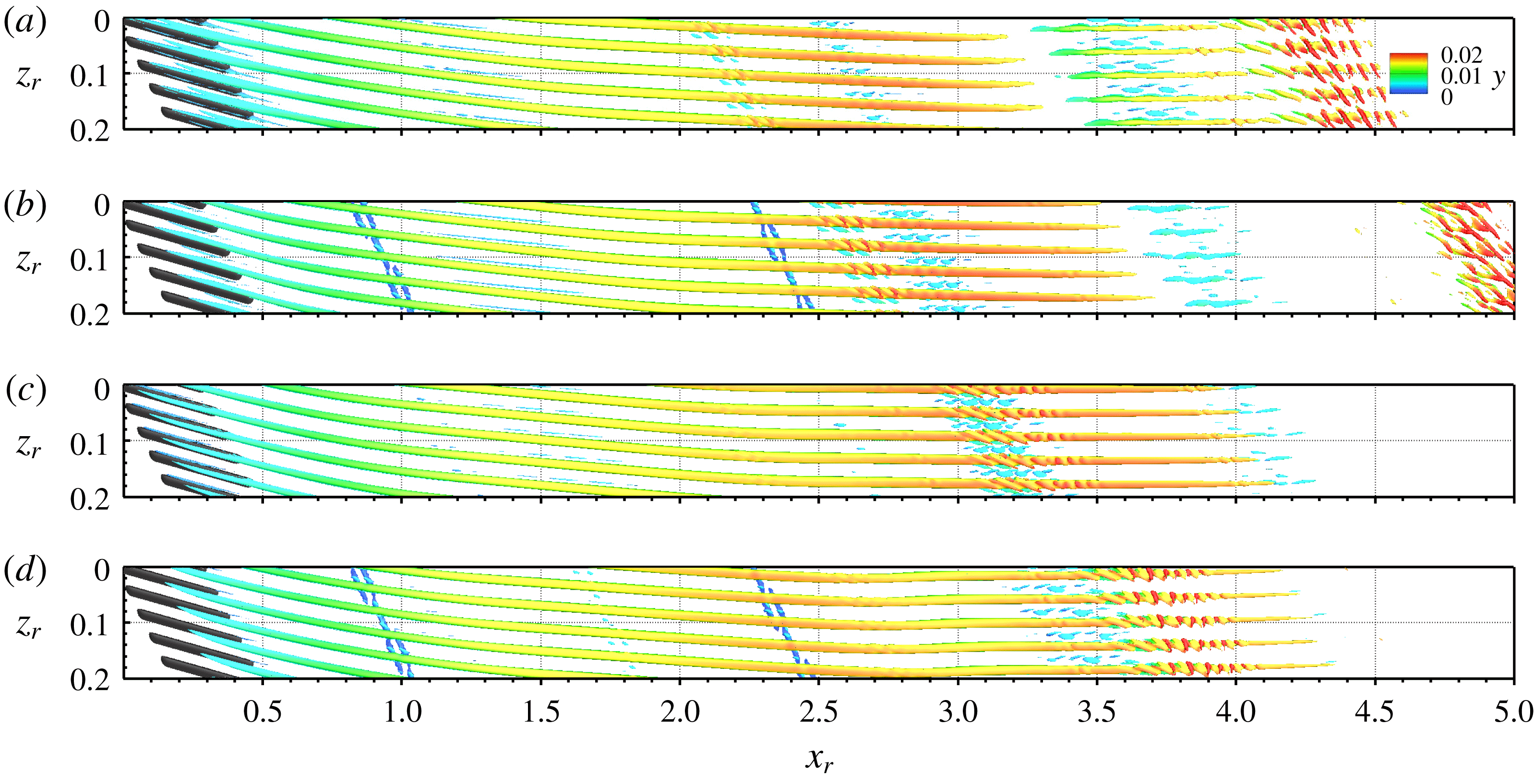
Figure 16(a–d) shows the vortical structures arising from the actuation at four time instances within one full excitation cycle (
 $\unicode[STIX]{x1D714}=3$
). The volume force attains the maximum at
$\unicode[STIX]{x1D714}=3$
). The volume force attains the maximum at
 $t=0.5T_{0}$
. In the vicinity of the actuators, unsteady CF vortices travelling in the positive
$t=0.5T_{0}$
. In the vicinity of the actuators, unsteady CF vortices travelling in the positive
 $z$
-direction are excited continuously. The vortex axes are mainly parallel to the electrode axis of the actuators and hence aligned with the wave front of the mode
$z$
-direction are excited continuously. The vortex axes are mainly parallel to the electrode axis of the actuators and hence aligned with the wave front of the mode
 $(0.5,+3)$
. Downstream of the actuator row up to
$(0.5,+3)$
. Downstream of the actuator row up to
 $x_{r}\approx 2.5$
, the vortical structures are quite similar to those in case BS-UFD-R due to the dominance of
$x_{r}\approx 2.5$
, the vortical structures are quite similar to those in case BS-UFD-R due to the dominance of
 $(0.5,+3)$
. Due to the growing steady mode
$(0.5,+3)$
. Due to the growing steady mode
 $(0,2)$
superposed onto the travelling mode, the main CF vortices break into isolated segments; see figure 16(a). Farther downstream, the primary CF vortices disappear and only some secondary structures far from the wall are visible.
$(0,2)$
superposed onto the travelling mode, the main CF vortices break into isolated segments; see figure 16(a). Farther downstream, the primary CF vortices disappear and only some secondary structures far from the wall are visible.
Spatial chordwise amplification rates
 $\unicode[STIX]{x1D6FC}_{i}$
of unstable CF-vortex modes for case PA-UFD in comparison to the corresponding base-flow data (lines with levels 0.0 to
$\unicode[STIX]{x1D6FC}_{i}$
of unstable CF-vortex modes for case PA-UFD in comparison to the corresponding base-flow data (lines with levels 0.0 to
 $-4.2$
,
$-4.2$
,
 $\unicode[STIX]{x1D6E5}=0.3$
). (a) Steady modes; the dashed lines mark the modes
$\unicode[STIX]{x1D6E5}=0.3$
). (a) Steady modes; the dashed lines mark the modes
 $(0,2)$
(lower) and
$(0,2)$
(lower) and
 $(0,3)$
(upper). (b) Unsteady modes with
$(0,3)$
(upper). (b) Unsteady modes with
 $\unicode[STIX]{x1D714}=6$
; the dashed lines mark the modes
$\unicode[STIX]{x1D714}=6$
; the dashed lines mark the modes
 $(1,+2)$
(lower) and
$(1,+2)$
(lower) and
 $(1,+3)$
(upper).
$(1,+3)$
(upper).
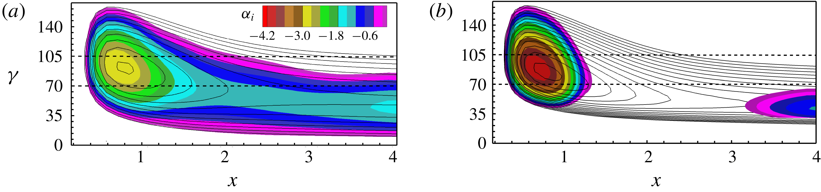
The stability diagrams gained by the time- and spanwise-averaged mean flow are shown in figure 17. Compared to case BS-UFD-R, the onset of the stabilizing effect occurs somewhat farther downstream due to the slightly lower initial amplitude of the UFD mode
 $(0.5,+3)$
. Different from the steady actuation investigated by Dörr & Kloker (Reference Dörr and Kloker2017), the unsteady volume force does not permanently counteract the CF. Hence, a direct modification of the stability properties in the vicinity of the actuators is not observed. Farther downstream, the stability properties basically coincide with those for case BS-UFD-R. Additional simulations with higher actuation strength but identical spatial force distribution (not shown) reveal enhanced stabilization for
$(0.5,+3)$
. Different from the steady actuation investigated by Dörr & Kloker (Reference Dörr and Kloker2017), the unsteady volume force does not permanently counteract the CF. Hence, a direct modification of the stability properties in the vicinity of the actuators is not observed. Farther downstream, the stability properties basically coincide with those for case BS-UFD-R. Additional simulations with higher actuation strength but identical spatial force distribution (not shown) reveal enhanced stabilization for
 $x<1.7$
but also higher amplitude level of the modes
$x<1.7$
but also higher amplitude level of the modes
 $(0,3)$
and
$(0,3)$
and
 $(0.5,-3)$
downstream, which possibly counteracts the UFD effect because of the stronger nonlinear interaction between steady and unsteady modes. Therefore, the sensitivity of the unsteady technique to detrimental ‘over’-actuation seems somewhat higher than that of the steady approach.
$(0.5,-3)$
downstream, which possibly counteracts the UFD effect because of the stronger nonlinear interaction between steady and unsteady modes. Therefore, the sensitivity of the unsteady technique to detrimental ‘over’-actuation seems somewhat higher than that of the steady approach.
4.3 Transition delay using travelling UFD modes excited by unsteady volume forcing
(a) Downstream development of modal
 $\tilde{u} _{s,(h,k)}^{\prime }$
and
$\tilde{u} _{s,(h,k)}^{\prime }$
and
 $\tilde{u} _{s,(h)}^{\prime }$
amplitudes from Fourier analysis (maximum over
$\tilde{u} _{s,(h)}^{\prime }$
amplitudes from Fourier analysis (maximum over
 $y$
or
$y$
or
 $y$
and
$y$
and
 $z$
,
$z$
,
 $6\leqslant \unicode[STIX]{x1D714}\leqslant 180$
,
$6\leqslant \unicode[STIX]{x1D714}\leqslant 180$
,
 $\unicode[STIX]{x0394}\unicode[STIX]{x1D714}=6$
) for case PA-UFD-S. The green rectangle indicates the chordwise position of the volume forcing. Open symbols denote the reference case. (b–e) Vortex visualization (snapshots,
$\unicode[STIX]{x0394}\unicode[STIX]{x1D714}=6$
) for case PA-UFD-S. The green rectangle indicates the chordwise position of the volume forcing. Open symbols denote the reference case. (b–e) Vortex visualization (snapshots,
 $\unicode[STIX]{x1D706}_{2}=-4$
, colour indicates
$\unicode[STIX]{x1D706}_{2}=-4$
, colour indicates
 $y$
) for case PA-UFD-S at
$y$
) for case PA-UFD-S at
 $t/T_{0}=$
(b) 16.5, (c) 17, (d) 17.5 and (e) 18 in the rotated (fixed) reference system according to (3.1). Note the compression of the
$t/T_{0}=$
(b) 16.5, (c) 17, (d) 17.5 and (e) 18 in the rotated (fixed) reference system according to (3.1). Note the compression of the
 $x_{r}$
-axis (
$x_{r}$
-axis (
 $z_{r}:x_{r}=2:1$
).
$z_{r}:x_{r}=2:1$
).
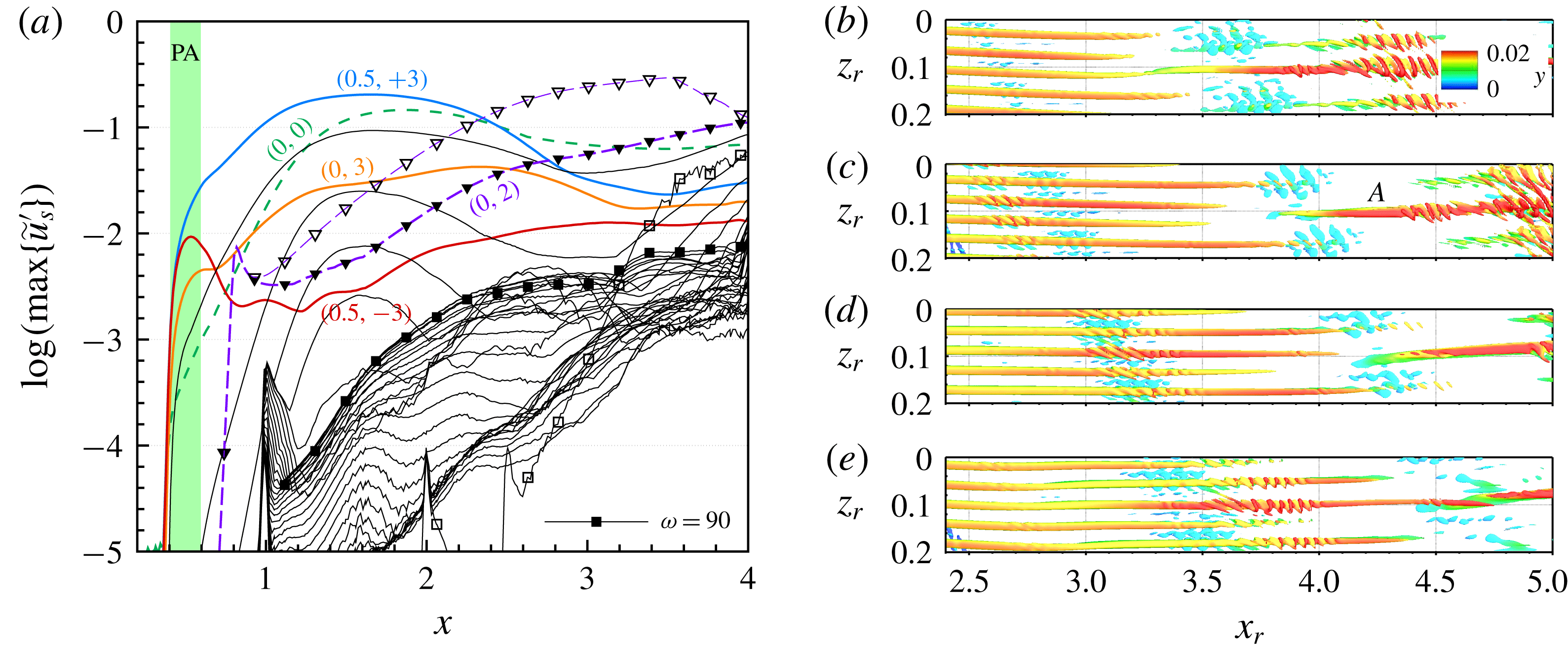
Like figure 18 but for case PA-UFD-U.

In cases PA-UFD-S and PA-UFD-U, the same volume-force actuation set-up as used for case PA-UFD is now employed to cases REF-S and REF-U, respectively. As shown in figures 18(a) and 19(a), for both cases, the downstream development of the UFD modes
 $(0.5,\pm 3)$
and
$(0.5,\pm 3)$
and
 $(0,3)$
and the mean-flow distortion
$(0,3)$
and the mean-flow distortion
 $(0,0)$
agrees exactly with that of case PA-UFD up to
$(0,0)$
agrees exactly with that of case PA-UFD up to
 $x\approx 2.3$
. In case PA-UFD-S, the test mode
$x\approx 2.3$
. In case PA-UFD-S, the test mode
 $(0,2)$
reaches an amplitude of 10 % only at
$(0,2)$
reaches an amplitude of 10 % only at
 $x=3.9$
, whereas this is at
$x=3.9$
, whereas this is at
 $x=2.2$
in the reference case REF-S. However, compared to the steady UFD approach investigated by Dörr & Kloker (Reference Dörr and Kloker2017) for the identical base flow, the growth attenuation is somewhat less effective. For
$x=2.2$
in the reference case REF-S. However, compared to the steady UFD approach investigated by Dörr & Kloker (Reference Dörr and Kloker2017) for the identical base flow, the growth attenuation is somewhat less effective. For
 $x>3.2$
, the low-frequency components of the perturbation spectrum are filled up progressively due to the interaction between the actuation-induced modes and the growing test mode
$x>3.2$
, the low-frequency components of the perturbation spectrum are filled up progressively due to the interaction between the actuation-induced modes and the growing test mode
 $(0,2)$
which attains a nonlinear amplitude. Compared to the reference case REF-S, the strong growth of the high-frequency secondary instability modes
$(0,2)$
which attains a nonlinear amplitude. Compared to the reference case REF-S, the strong growth of the high-frequency secondary instability modes
 $\unicode[STIX]{x1D714}\approx 90$
induced by the mode
$\unicode[STIX]{x1D714}\approx 90$
induced by the mode
 $(0,2)$
is distinctly attenuated, and the transition does not occur in the considered domain. In case PA-UFD-U, the amplification of the test mode
$(0,2)$
is distinctly attenuated, and the transition does not occur in the considered domain. In case PA-UFD-U, the amplification of the test mode
 $(1,+2)$
is virtually completely suppressed, and consequently the secondary instability.
$(1,+2)$
is virtually completely suppressed, and consequently the secondary instability.
In physical space, the vortical structures arising for case PA-UFD-S for
 $x_{r}<2.5$
are virtually identical to those appearing in case PA-UFD without test mode (not shown). Farther downstream, as shown in figure 18(b,e), the oncoming CF vortices, mainly associated with the dominating UFD mode
$x_{r}<2.5$
are virtually identical to those appearing in case PA-UFD without test mode (not shown). Farther downstream, as shown in figure 18(b,e), the oncoming CF vortices, mainly associated with the dominating UFD mode
 $(0.5,+3)$
, are strongly detuned due to the modulation by the nonlinear steady mode
$(0.5,+3)$
, are strongly detuned due to the modulation by the nonlinear steady mode
 $(0,2)$
. For
$(0,2)$
. For
 $x_{r}>3.5$
, a distinct CF vortex
$x_{r}>3.5$
, a distinct CF vortex
 $A$
detaches from the oncoming CF vortex and keeps growing whereas other primary structures fade out. Being supported by
$A$
detaches from the oncoming CF vortex and keeps growing whereas other primary structures fade out. Being supported by
 $A$
, the complex secondary structures in figure 18(c) at the end of the visualized region may finally evolve into turbulent spots farther downstream. For case PA-UFD-U, as expected, the vortical structures are identical to those of case PA-UFD due to the completely suppressed test mode; see figure 19(b–e).
$A$
, the complex secondary structures in figure 18(c) at the end of the visualized region may finally evolve into turbulent spots farther downstream. For case PA-UFD-U, as expected, the vortical structures are identical to those of case PA-UFD due to the completely suppressed test mode; see figure 19(b–e).
As for a combined steady/unsteady test-modes scenario the following holds. Once a dominating mode becomes nonlinear (
 ${>}$
5 %), the amplification of other primary modes is suppressed; see Bonfigli & Kloker (Reference Bonfigli and Kloker1999). If both steady and unsteady modes reach nonlinear amplitudes simultaneously, the transition is promoted by strong nonlinear interaction. This complex scenario was investigated in detail by Bonfigli & Kloker (Reference Bonfigli and Kloker2005). An additional simulation with the control actuator (case ‘PA-UFD-S
${>}$
5 %), the amplification of other primary modes is suppressed; see Bonfigli & Kloker (Reference Bonfigli and Kloker1999). If both steady and unsteady modes reach nonlinear amplitudes simultaneously, the transition is promoted by strong nonlinear interaction. This complex scenario was investigated in detail by Bonfigli & Kloker (Reference Bonfigli and Kloker2005). An additional simulation with the control actuator (case ‘PA-UFD-S
 $+$
U’, not shown) reveals that also in this case the travelling mode
$+$
U’, not shown) reveals that also in this case the travelling mode
 $(1,+2)$
is damped out by the unsteady UFD and the resulting flow field is quite similar to that of case PA-UFD-S.
$(1,+2)$
is damped out by the unsteady UFD and the resulting flow field is quite similar to that of case PA-UFD-S.
To quantify the reduction of the skin-friction drag achieved, the wall-normal gradient of the mean velocity component in the direction of the oncoming flow at the wall is calculated, which is proportional to the local skin-friction coefficient. The mean velocity in the direction of the oncoming flow is denoted as
 $u_{41^{\circ }}$
, where
$u_{41^{\circ }}$
, where
 $41^{\circ }$
is the effective sweep angle of the plate. Results of the controlled cases are compared with the corresponding steady or unsteady reference cases; see figures 20(a) and 20(c), respectively. Due to the presence of the nonlinear UFD mode in the controlled cases, the wall-normal gradient is increased in the upstream region. However, due to the delayed transition, the sharp rise of the wall-normal gradient as found for case REF-S at
$41^{\circ }$
is the effective sweep angle of the plate. Results of the controlled cases are compared with the corresponding steady or unsteady reference cases; see figures 20(a) and 20(c), respectively. Due to the presence of the nonlinear UFD mode in the controlled cases, the wall-normal gradient is increased in the upstream region. However, due to the delayed transition, the sharp rise of the wall-normal gradient as found for case REF-S at
 $x\approx 3.5$
and for case REF-U at
$x\approx 3.5$
and for case REF-U at
 $x\approx 3.2$
does not occur. The chordwise integrated value at the end of the domain in both controlled cases is significantly lowered; see figures 20(b) and 20(d), respectively.
$x\approx 3.2$
does not occur. The chordwise integrated value at the end of the domain in both controlled cases is significantly lowered; see figures 20(b) and 20(d), respectively.
Downstream development of the (a,c) wall-normal gradient and (b,d) chordwise direction integrated wall-normal gradient of the spanwise mean velocity component in the direction of the oncoming flow at the wall. For the integration, the maximum value over one fundamental period is used to account for a fully turbulent flow.
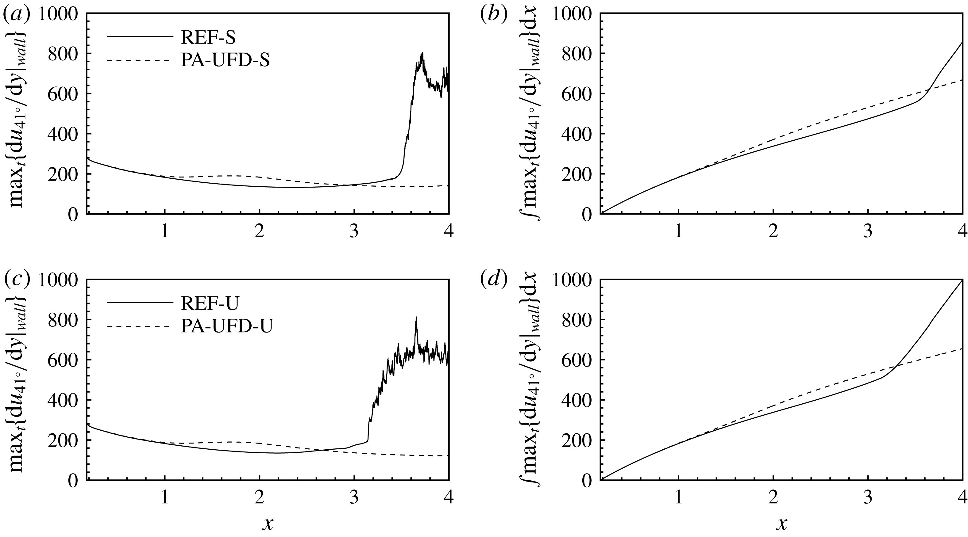
5 Conclusions
An unsteady UFD technique to delay the CF-induced transition in a three-dimensional swept-wing-type boundary layer has been investigated by DNS. Suction/blowing or volume-force actuators have been employed, the latter mimicking alternating-current dielectric-barrier-discharge plasma actuators. The volume force is varied by a low-frequency sinusoidal modulating signal, imitating the inherent unsteadiness of the plasma actuation, but also has a small steady part.
The effect of single travelling CF-vortex modes with a spanwise wavelength two-thirds that of the most amplified mode
 $(1,+2)$
, excited by a blowing/suction strip, has been investigated at first. It has been shown that the low-frequency modes
$(1,+2)$
, excited by a blowing/suction strip, has been investigated at first. It has been shown that the low-frequency modes
 $(0.5,\pm 3)$
cause primary CF vortices travelling in opposite spanwise directions with slightly different axis orientations. Different three-dimensional flow patterns result in qualitatively different secondary instability behaviours of the background disturbances. The rightward-travelling mode
$(0.5,\pm 3)$
cause primary CF vortices travelling in opposite spanwise directions with slightly different axis orientations. Different three-dimensional flow patterns result in qualitatively different secondary instability behaviours of the background disturbances. The rightward-travelling mode
 $(0.5,+3)$
invokes only very limited growth of high-frequency type-I and type-II modes in a short region. The low-frequency type-III modes triggered by the leftward-travelling mode
$(0.5,+3)$
invokes only very limited growth of high-frequency type-I and type-II modes in a short region. The low-frequency type-III modes triggered by the leftward-travelling mode
 $(0.5,-3)$
undergo a strong amplification, altering the shear layers in the near-wall region and leading to an unwanted strong increase of the disturbance level. We found that both modes
$(0.5,-3)$
undergo a strong amplification, altering the shear layers in the near-wall region and leading to an unwanted strong increase of the disturbance level. We found that both modes
 $(0.5,\pm 3)$
generate a beneficial mean-flow distortion, stabilizing the flow with respect to the otherwise most amplified steady and unsteady CF-vortex modes. However, control mode
$(0.5,\pm 3)$
generate a beneficial mean-flow distortion, stabilizing the flow with respect to the otherwise most amplified steady and unsteady CF-vortex modes. However, control mode
 $(0.5,-3)$
, running with the basic CF, is ruled out because of giving rise to detrimental secondary instability.
$(0.5,-3)$
, running with the basic CF, is ruled out because of giving rise to detrimental secondary instability.
Using three volume-force actuators per fundamental wavelength operated with a frequency of
 $\unicode[STIX]{x1D714}_{PA}=3$
, where
$\unicode[STIX]{x1D714}_{PA}=3$
, where
 $\unicode[STIX]{x1D714}=6$
is that of the most amplified mode, the travelling CF-vortex modes
$\unicode[STIX]{x1D714}=6$
is that of the most amplified mode, the travelling CF-vortex modes
 $(0.5,\pm 3)$
are simultaneously triggered in the boundary layer. Turning the actuators’ axes to align with the wave crests of the target mode
$(0.5,\pm 3)$
are simultaneously triggered in the boundary layer. Turning the actuators’ axes to align with the wave crests of the target mode
 $(0.5,+3)$
, its receptivity is maximized and the formation of other misaligned modes is substantially abated. The unavoidable forcing of the steady mode
$(0.5,+3)$
, its receptivity is maximized and the formation of other misaligned modes is substantially abated. The unavoidable forcing of the steady mode
 $(0,3)$
could be also minimized.
$(0,3)$
could be also minimized.
At controlling steady test modes, transition is significantly delayed by reducing the primary growth of the integrally most amplified steady CF-vortex mode. Compared to the steady UFD method using
 $(0,3)$
as control mode, the growth attenuation of the test mode
$(0,3)$
as control mode, the growth attenuation of the test mode
 $(0,2)$
is somewhat weaker. The nonlinear interaction between the growing steady test modes and the unsteady UFD mode diminishes the beneficial effect of the UFD. The control of unsteady test modes turns out to be more effective, as the primary growth of the test mode
$(0,2)$
is somewhat weaker. The nonlinear interaction between the growing steady test modes and the unsteady UFD mode diminishes the beneficial effect of the UFD. The control of unsteady test modes turns out to be more effective, as the primary growth of the test mode
 $(1,+2)$
has been virtually completely suppressed.
$(1,+2)$
has been virtually completely suppressed.
If plasma actuators are used for CF transition control in the UFD mode, because they can be seen as tunable ‘roughness’ with controllable strength and also possibly controllable spanwise spacing, the energy consumption still may play a role. This consumption can be significantly reduced with respect to the steady UFD approach since the inherent unsteady fluctuating part of the plasma-induced volume force is exploited; also, unsteady CF-vortex modes are more strongly amplified and need smaller initial amplitudes. Furthermore, unlike the steady UFD approach, with these actuators an operating frequency clearly outside the unstable frequency range of the flow is not required. Hence, the unsteady approach may open opportunities for employing plasma-based control devices at higher free-stream velocities.
Acknowledgements
The provision of computational resources on the national supercomputer Cray XC40 at the Federal High Performance Computing Center Stuttgart (HLRS) under grant GCS-Lamt, ID
 $=$
44026, is gratefully acknowledged, as is the fellowship from the China Scholarship Council (CSC) for Z.G.
$=$
44026, is gratefully acknowledged, as is the fellowship from the China Scholarship Council (CSC) for Z.G.


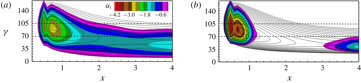

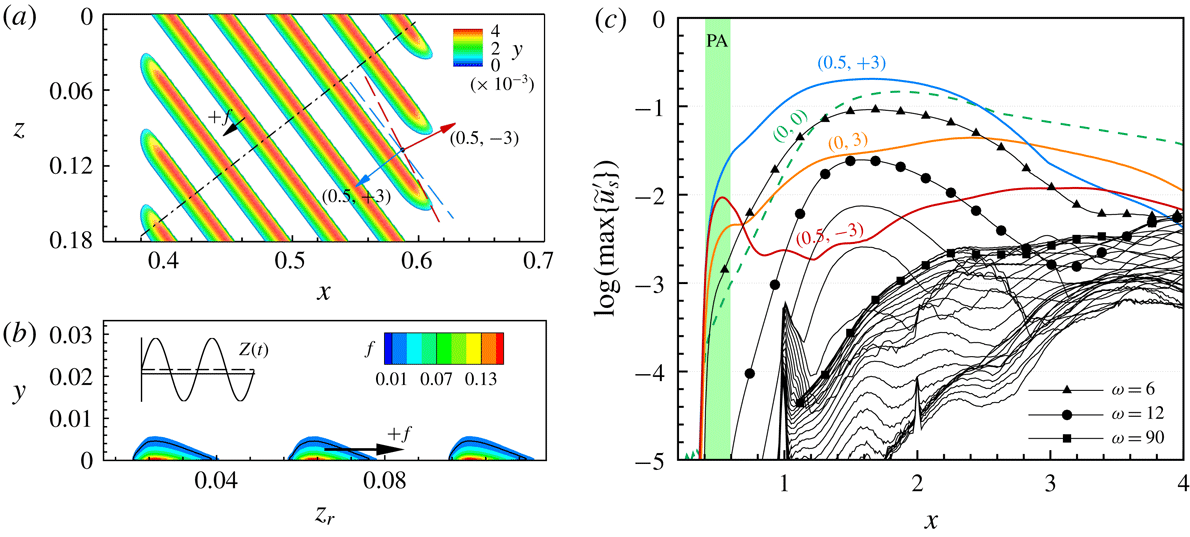


 Open access