


1 Introduction
Extremal black holes are special solutions of Einstein’s equations of general relativity which have absolute zero temperature in the celebrated thermodynamic analogy of black hole mechanics. The simplest examples of extremal black holes are given by the extremal Reissner–Nordström (ERN) metrics
 $$ \begin{align} g_{\mathrm{ERN}}\doteq -\left(1-\frac{M}{r}\right)^2dt^2+\left(1-\frac{M}{r}\right)^{-2}dr^2+r^2(d\vartheta^2+\sin^2\vartheta\,d\varphi^2), \end{align} $$
where M is a positive parameter known as the mass. The metric (1.1) solves the Einstein–Maxwell equations,
 $$ \begin{align} R_{\mu\nu}-\tfrac 12 Rg_{\mu\nu} = 2F_{\mu\alpha}F_\nu{}^{\alpha}-\tfrac 12 g_{\mu\nu}F_{\alpha\beta}F^{\alpha\beta}\quad\text{and}\quad \nabla_\mu F^{\mu\nu}=0, \end{align} $$
and is spherically symmetric, asymptotically flat, and static, with time-translation Killing vector field
 $T\doteq \partial _t$
.
$T\doteq \partial _t$
.
The extremal Reissner–Nordström metrics (1.1) arise as an exceptional one-parameter subfamily of the full Reissner–Nordström family [Reference Reissner62, Reference Nordström59] of solutions to the Einstein–Maxwell equations,
 $$ \begin{align} g_{M,e}\doteq -\left(1-\frac{2M}{r}+\frac{e^2}{r^2}\right)dt^2+\left(1-\frac{2M}{r}+\frac{e^2}{r^2}\right)^{-1}dr^2+r^2(d\vartheta^2+\sin^2\vartheta\,d\varphi^2), \end{align} $$
where e is a real parameter representing the charge of the electromagnetic field. The extremal case corresponds to the parameter values
 $|e|=M$
. For the parameter range
$|e|=M$
. For the parameter range
 $|e|\le M$
, the metric
$|e|\le M$
, the metric
 $g_{M,e}$
describes a black hole spacetime. When
$g_{M,e}$
describes a black hole spacetime. When
 $|e|<M$
, the solution is called subextremal, and the
$|e|<M$
, the solution is called subextremal, and the
 $|e|=M$
case corresponds to the extremal Reissner–Nordström metric (1.1) above. When
$|e|=M$
case corresponds to the extremal Reissner–Nordström metric (1.1) above. When
 $e=0$
,
$e=0$
,
 $g_{M,e}$
reduces to the celebrated Schwarzschild solution [Reference Schwarzschild65] of the Einstein vacuum equations. When
$g_{M,e}$
reduces to the celebrated Schwarzschild solution [Reference Schwarzschild65] of the Einstein vacuum equations. When
 $|e|>M$
, the superextremal case, the metric
$|e|>M$
, the superextremal case, the metric
 $g_{M,e}$
no longer describes a black hole. The role of superextremality will be discussed in Section 1.3 below.
$g_{M,e}$
no longer describes a black hole. The role of superextremality will be discussed in Section 1.3 below.
For any of the Reissner–Nordström black hole spacetimes, the Killing field satisfies
 $$ \begin{align} \nabla_TT|_{\mathcal H^+}=\varkappa T|_{\mathcal H^+}, \end{align} $$
where
 $\mathcal H^+$
denotes the event horizon, the boundary of the black hole region. The number
$\mathcal H^+$
denotes the event horizon, the boundary of the black hole region. The number
 $\varkappa =\varkappa (M,e)$
, called the surface gravity of
$\varkappa =\varkappa (M,e)$
, called the surface gravity of
 $\mathcal H^+$
, is given by
$\mathcal H^+$
, is given by
 $$ \begin{align*} \varkappa(M,e)\doteq \frac{\sqrt{M^2-e^2}}{(M+\sqrt{M^2-e^2})^2} \end{align*} $$
and quantifies the celebrated horizon redshift effect: the null generators of
 $\mathcal H^+$
have exponentially decaying energy, with rate determined by
$\mathcal H^+$
have exponentially decaying energy, with rate determined by
 $\varkappa $
(see for instance [Reference Sbierski63]).
$\varkappa $
(see for instance [Reference Sbierski63]).
The event horizon of subextremal Reissner–Nordström has
 $\varkappa>0$
, while the event horizon of extremal Reissner–Nordström has
$\varkappa>0$
, while the event horizon of extremal Reissner–Nordström has
 $\varkappa =0$
, a distinction which has fundamental repercussions for the behavior of perturbations of these spacetimes. In the seminal work [Reference Dafermos and Rodnianski29], Dafermos and Rodnianski proved the nonlinear asymptotic stability of the subextremal Reissner–Nordström family as solutions of the Einstein–Maxwell equations coupled to a neutral scalar field in spherical symmetry. The horizon redshift effect is central to [Reference Dafermos and Rodnianski29] and is a cornerstone of our understanding of linear waves on subextremal Reissner–Nordström black holes without symmetry assumptions [Reference Dafermos and Rodnianski30, Reference Dafermos and Rodnianski32]. By the work of Dafermos–Holzegel–Rodnianski [Reference Dafermos, Holzegel and Rodnianski26] and Blue [Reference Blue15] (see also [Reference Pasqualotto60]) for
$\varkappa =0$
, a distinction which has fundamental repercussions for the behavior of perturbations of these spacetimes. In the seminal work [Reference Dafermos and Rodnianski29], Dafermos and Rodnianski proved the nonlinear asymptotic stability of the subextremal Reissner–Nordström family as solutions of the Einstein–Maxwell equations coupled to a neutral scalar field in spherical symmetry. The horizon redshift effect is central to [Reference Dafermos and Rodnianski29] and is a cornerstone of our understanding of linear waves on subextremal Reissner–Nordström black holes without symmetry assumptions [Reference Dafermos and Rodnianski30, Reference Dafermos and Rodnianski32]. By the work of Dafermos–Holzegel–Rodnianski [Reference Dafermos, Holzegel and Rodnianski26] and Blue [Reference Blue15] (see also [Reference Pasqualotto60]) for
 $e=0$
and Giorgi [Reference Giorgi38, Reference Giorgi39] for
$e=0$
and Giorgi [Reference Giorgi38, Reference Giorgi39] for
 $|e|<M$
, subextremal Reissner–Nordström is now known to be linearly stable in Einstein–Maxwell theory outside of symmetry.
$|e|<M$
, subextremal Reissner–Nordström is now known to be linearly stable in Einstein–Maxwell theory outside of symmetry.
The theory of linear waves on extremal black holes – and by extension, nonlinear perturbations of extremal black holes – is very different. In a remarkable series of papers [Reference Aretakis10, Reference Aretakis11, Reference Aretakis13], Aretakis showed that ingoing null derivatives of solutions to the linear wave equation on extremal Reissner–Nordström – even those arising from well-localized initial data – generically do not decay on the event horizon, and higher derivatives may even grow polynomially in time. This horizon instability for the linear wave equation, which has become known as the Aretakis instability, has also been extended to gravitational perturbations [Reference Lucietti, Murata, Reall and Tanahashi52, Reference Apetroaie8] of extremal Reissner–Nordström and to axisymmetric linear waves on extremal Kerr [Reference Aretakis12, Reference Lucietti and Reall53]. Gajic has recently shown that extremal Kerr is subject to additional stronger instabilities arising from higher azimuthal modes [Reference Gajic35] (see also the earlier heuristic analysis [Reference Casals, Gralla and Zimmerman16]), which will be discussed further in Section 1.4.2 below.
These horizon instabilities (along with the specter of superextremality which we will address in Section 1.3 below) present a substantial obstacle to understanding the moduli space of solutions to the Einstein equations near extremal Reissner–Nordström, Kerr, and Kerr–Newman black holes. In a pioneering numerical study [Reference Murata, Reall and Tanahashi58], Murata, Reall, and Tanahashi studied spherically symmetric perturbations of extremal Reissner–Nordström in the Einstein–Maxwell-neutral scalar field model and observed that the Aretakis instability for the scalar field is still activated on the dynamical background, but that the geometry is not completely disrupted in the process. These numerical results and rigorous work on nonlinear model problems by the first-named author, Aretakis, and Gajic [Reference Angelopoulos1, Reference Angelopoulos, Aretakis and Gajic3, Reference Angelopoulos, Aretakis and Gajic7], have given rise to the hope that extremal Reissner–Nordström could be stable in spite of the Aretakis instability; see [Reference Dafermos, Holzegel, Rodnianski and Taylor27, Conjecture IV.2] and the recent essay by Dafermos [Reference Dafermos25].
1.1 Stability and instability of extremal Reissner–Nordström for the spherically symmetric Einstein–Maxwell-neutral scalar field system
In this paper, we initiate the rigorous study of the (in)stability properties of extremal Reissner–Nordström black holes as solutions to the full nonlinear Einstein field equations. We work with the spherically symmetric Einstein–Maxwell-neutral scalar field model, which is the same model as in Murata–Reall–Tanahashi [Reference Murata, Reall and Tanahashi58] (and has been used in other influential works in recent years [Reference Dafermos21, Reference Dafermos22, Reference Dafermos and Rodnianski29, Reference Luk and Oh55]). This system consists of a spherically symmetric, charged spacetime
 $(\mathcal M^{3+1},g,F)$
together with a spherically symmetric massless scalar field
$(\mathcal M^{3+1},g,F)$
together with a spherically symmetric massless scalar field
 $\phi :\mathcal M\to \mathbb R$
satisfying the linear wave equation
$\phi :\mathcal M\to \mathbb R$
satisfying the linear wave equation
 $$ \begin{align} \Box_g\phi=0 \end{align} $$
on the dynamical background, with total energy-momentum tensor given by
 $$ \begin{align*} T_{\mu\nu}\doteq F_{\mu\alpha}F_\nu{}^\alpha-\tfrac 14 g_{\mu\nu}F_{\alpha\beta}F^{\alpha\beta}+\partial_\mu\phi\partial_\nu\phi -\tfrac 12g_{\mu\nu}\partial_\alpha\phi\partial^\alpha\phi. \end{align*} $$
This is one of the simplest self-gravitating models in which one can entertain dynamical nonlinear perturbations of Reissner–Nordström, as a toy model for the electro-vacuum equations. See already Section 2.1 for the precise definitions and equations of the model.
We now state rough versions of our main theorems; the detailed statements and associated definitions will be presented in Section 3 below.
Theorem I (Codimension-one nonlinear stability of ERN, rough version).
Let
 ${\mathfrak{M}}$
denote the moduli space of characteristic data for the spherically symmetric Einstein–Maxwell-neutral scalar field system posed on a bifurcate null hypersurface
${\mathfrak{M}}$
denote the moduli space of characteristic data for the spherically symmetric Einstein–Maxwell-neutral scalar field system posed on a bifurcate null hypersurface
 $C_{\mathrm{out}}\cup \underline C{}_{\mathrm{in}}$
, as in Fig. 1 below, which lie close to extremal Reissner–Nordström in an appropriate norm. There exists a “codimension-one submanifold”
$C_{\mathrm{out}}\cup \underline C{}_{\mathrm{in}}$
, as in Fig. 1 below, which lie close to extremal Reissner–Nordström in an appropriate norm. There exists a “codimension-one submanifold”
 ${\mathfrak{M}}_{\mathrm{stab}}\subset {\mathfrak{M}}$
such that any data in
${\mathfrak{M}}_{\mathrm{stab}}\subset {\mathfrak{M}}$
such that any data in
 ${\mathfrak{M}}_{\mathrm{stab}}$
evolve into a spacetime with the following properties:
${\mathfrak{M}}_{\mathrm{stab}}$
evolve into a spacetime with the following properties:
-
(i) Future null infinity
 $\mathcal I^+$
is complete and the causal past of future null infinity,
$J^-(\mathcal I^+)$
, is bounded by a regular event horizon
$\mathcal H^+$
, which itself bounds a nonempty black hole region
$\mathcal {BH}\doteq \mathcal M\setminus J^-(\mathcal I^+)$
.
$\mathcal I^+$
is complete and the causal past of future null infinity,
$J^-(\mathcal I^+)$
, is bounded by a regular event horizon
$\mathcal H^+$
, which itself bounds a nonempty black hole region
$\mathcal {BH}\doteq \mathcal M\setminus J^-(\mathcal I^+)$
. -
(ii) The metric remains close to the initial extremal Reissner–Nordström metric in the domain of outer communication and appropriately defined energy fluxes and pointwise
$C^1$
norms of the scalar field
$\phi $
are bounded in terms of their initial data on
$C_{\mathrm{out}}\cup \underline C{}_{\mathrm{in}}$
. -
(iii) The metric decays polynomially in
$C^0$
(as an appropriate notion of “time” tends to infinity) to a nearby member of the extremal Reissner–Nordström family, relative to a teleologically defined double null gauge uniformly in the entire domain of outer communication. The renormalized Hawking mass (see already Section 2.1.1) converges uniformly to the final mass of the black hole. The scalar field decays polynomially to zero pointwise and in an appropriate energy norm. -
(iv) The spacetime does not contain strictly trapped surfaces. Any marginally trapped surfaces lie on the event horizon
$\mathcal H^+$
.


A Penrose diagram showing the maximal development of a solution considered in Theorem I. The Cauchy data ends on the left at the solid point, where it is incomplete (but not singular).

Some comments about this statement are in order:
-
1. Because the extremal Reissner–Nordström family is already codimension-one within the full Reissner–Nordström family, any stability statement for it is necessarily a positive codimension statement, with codimension one being sharp. This aspect of the problem is familiar from the proof of nonlinear stability of Schwarzschild outside of symmetry by Dafermos, Holzegel, Rodnianski, and Taylor [Reference Dafermos, Holzegel, Rodnianski and Taylor27]. For conjectures regarding the regularity of
${\mathfrak{M}}_{\mathrm{stab}}$
and what happens “on either side” of it, see already Section 1.3. -
2. The theorem states that the metric decays in
$C^0$
(and some Christoffel symbols) to that of extremal Reissner–Nordström and that the scalar field decays in
$C^0$
to zero. We will show in Theorem II below that the metric does not necessarily decay to extremal Reissner–Nordström in
$C^2$
(and may grow in
$C^3$
) and that the scalar field does not necessarily decay in
$C^1$
(and may grow in
$C^2$
). -
3. The norms and decay rates for the scalar field
$\phi $
are consistent with the norms and decay rates for spherically symmetric solutions of the linear wave equation on extremal Reissner–Nordström. We do not need to commute in order to close our bootstrap assumptions and hence do not prove sharp decay rates for
$\phi $
everywhere. See already Sections 1.2 and 1.4.1. -
4. Since we show that there are no trapped surfaces behind the event horizon, we in fact prove that the maximal development of data in
${\mathfrak{M}}_{\mathrm{stab}}$
is the full double null rectangle depicted in Fig. 1. For the behavior of the scalar field and geometry in the black hole interior, see already Section 1.3.2.


Our second main theorem shows that the Aretakis instability of the event horizon, i.e., nondecay of the first transverse derivative and linear growth of the second transverse derivative, persists in the Einstein–Maxwell-scalar field model. Moreover, in this coupled model, the instability affects the geometry as well.
Before stating the theorem, we recall briefly some features of the geometry of extremal Reissner–Nordström black holes. Let Y denote the coordinate vector field
 $\partial _r$
in ingoing Eddington–Finkelstein coordinates
$\partial _r$
in ingoing Eddington–Finkelstein coordinates
 $(v,r,\vartheta ,\varphi )$
. This null vector field is translation-invariant and transverse to the event horizon. Moreover, it is canonical in the sense that for any spherically symmetric double null coordinates
$(v,r,\vartheta ,\varphi )$
. This null vector field is translation-invariant and transverse to the event horizon. Moreover, it is canonical in the sense that for any spherically symmetric double null coordinates
 $(u,v,\vartheta ,\varphi )$
on extremal Reissner–Nordström with u “ingoing,” Y can be written as
$(u,v,\vartheta ,\varphi )$
on extremal Reissner–Nordström with u “ingoing,” Y can be written as
 $(\partial _ur)^{-1}\partial _u$
. The
$(\partial _ur)^{-1}\partial _u$
. The
 $YY$
-component of the Ricci tensor,
$YY$
-component of the Ricci tensor,
 $R_{YY}$
, vanishes identically on any Reissner–Nordström solution.
$R_{YY}$
, vanishes identically on any Reissner–Nordström solution.
Theorem II (Dynamical horizon instability, rough version).
For any initial data lying in
 ${\mathfrak{M}}_{\mathrm{stab}}$
, the following holds on the event horizon
${\mathfrak{M}}_{\mathrm{stab}}$
, the following holds on the event horizon
 $\mathcal H^+$
of its maximal globally hyperbolic development:
$\mathcal H^+$
of its maximal globally hyperbolic development:
-
(i) Let
$Y\doteq (\partial _ur)^{-1}\partial _u$
denote the gauge-invariant null derivative transverse to
$\mathcal H^+$
, where r is the area-radius of the spacetime, and u is a retarded time coordinate, i.e., increasing towards the black hole. Then
$R_{YY}$
and
$Y(r\phi )$
are approximately constant on
$\mathcal H^+$
, i.e., do not necessarily decay. -
(ii) There exists a relatively open subset of
${\mathfrak{M}}_{\mathrm{stab}}$
for which the “asymptotic Aretakis charge” (1.6)is nonvanishing. Here v is an advanced time coordinate on the spacetime such that
$$ \begin{align} H_0[\phi]\doteq \lim_{v\to\infty}Y(r\phi)|_{\mathcal H^+}(v) \end{align} $$
$v=\infty $
at future timelike infinity
$i^+$
. It holds that (1.7)
$$ \begin{align} \lim_{v\to\infty}R_{YY}|_{\mathcal H^+}(v)= 2M^{-2}\big(H_0[\phi]\big)^2. \end{align} $$
-
(iii) If
$H_0[\phi ]\ne 0$
, then there exists a constant
$c>0$
such that (1.8)
$$ \begin{align} \big|\nabla_YR_{YY}|_{\mathcal H^+}(v)\big|\ge cv,\qquad \big|Y^2(r\phi)|_{\mathcal H^+} (v)\big|\ge cv. \end{align} $$


As was mentioned before, the problem considered here was previously investigated numerically by Murata, Reall, and Tanahashi in [Reference Murata, Reall and Tanahashi58]. Theorems I and II rigorously confirm all of their findings about the black hole exterior and event horizon for initial data in
 ${\mathfrak{M}}_{\mathrm{stab}}$
and make precise the nature of the “fine tuning” required to asymptote to extremality. Their findings about the black hole interior at extremality are also verified by combining Theorem I with the work of Gajic and Luk [Reference Gajic and Luk36]; see already Section 1.3.2.
${\mathfrak{M}}_{\mathrm{stab}}$
and make precise the nature of the “fine tuning” required to asymptote to extremality. Their findings about the black hole interior at extremality are also verified by combining Theorem I with the work of Gajic and Luk [Reference Gajic and Luk36]; see already Section 1.3.2.
Remark 1.1. The nondecay and growth of
 $R_{YY}$
and
$R_{YY}$
and
 $\nabla _YR_{YY}$
along
$\nabla _YR_{YY}$
along
 $\mathcal H^+$
found in the present paper is distinct from the nondecay and growth of
$\mathcal H^+$
found in the present paper is distinct from the nondecay and growth of
 $\underline \alpha $
and
$\underline \alpha $
and ![]() found by Apetroaie in [Reference Apetroaie8] for the generalized Teukolsky system on extremal Reissner–Nordström, where
found by Apetroaie in [Reference Apetroaie8] for the generalized Teukolsky system on extremal Reissner–Nordström, where
 $\underline \alpha {}_{AB}\doteq W(e_A,Y,e_B,Y)$
, where W is the Weyl tensor, and
$\underline \alpha {}_{AB}\doteq W(e_A,Y,e_B,Y)$
, where W is the Weyl tensor, and
 $\{e_A\}_{A=1,2}$
span the symmetry spheres. Indeed,
$\{e_A\}_{A=1,2}$
span the symmetry spheres. Indeed,
 $\underline \alpha $
vanishes identically for a spherically symmetric metric.
$\underline \alpha $
vanishes identically for a spherically symmetric metric.
In this paper, we do not pursue the interesting question of which other geometric quantities exhibit instabilities at higher orders of differentiability.
1.2 Overview of the proof
The proof of Theorem I involves a bootstrap argument with a teleologically normalized double null gauge coupled to a discrete modulation argument performed on dyadic timescales. Theorem II is proved by combining the method of characteristics for the wave equation for
 $\phi $
with precise estimates on the dynamical degenerate redshift factor along the event horizon
$\phi $
with precise estimates on the dynamical degenerate redshift factor along the event horizon
 $\mathcal H^+$
. We now describe the proofs in some detail, beginning with the relevant theory for the linear wave equation on extremal Reissner–Nordström.
$\mathcal H^+$
. We now describe the proofs in some detail, beginning with the relevant theory for the linear wave equation on extremal Reissner–Nordström.
1.2.1 Review of spherically symmetric linear waves on extremal Reissner–Nordström and the Aretakis instability
Here we briefly review the theory of spherically symmetric solutions to the linear wave equation (1.5) on extremal Reissner–Nordström. Aretakis initiated the study of this problem in [Reference Aretakis10, Reference Aretakis11] but we will make use of technical advances made by the first-named author, Aretakis, and Gajic in [Reference Angelopoulos, Aretakis and Gajic5, Reference Angelopoulos, Aretakis and Gajic4, Reference Angelopoulos, Aretakis and Gajic6]. For a brief review of the geometry of extremal Reissner–Nordström, we refer the reader to Section 2.2 of the present paper, [Reference Aretakis10, Section 2], and the appendix of [Reference Aretakis9].
The general strategy to prove energy decay statements for waves on extremal Reissner–Nordström consists of, as in the subextremal case, deriving a hierarchy of weighted energy boundedness inequalities and time-integrated energy decay estimates. This hierarchy takes the form
 $$ \begin{align} &\int_{C(\tau_2)}r^p(\partial_v\psi)^2\, dv+ \int_{\underline C(\tau_2)} (r-M)^{2-p} \frac{(\partial_u\psi)^2}{-\partial_ur}\,du \nonumber\\& \quad\lesssim \int_{C(\tau_1)}r^p(\partial_v\psi)^2\, dv+ \int_{\underline C(\tau_1)} (r-M)^{2-p} \frac{(\partial_u\psi)^2}{-\partial_ur}\,du+\mathrm{l.o.t.}, \end{align} $$
 $$ \begin{align} \int_{\tau_1}^{\tau_2}\int_{C(\tau)} r^{p-1}(\partial_v\psi)^2\, dvd\tau&\lesssim \int_{C(\tau_1)}r^p(\partial_v\psi)^2\, dv + \text{l.o.t.}, \end{align} $$
 $$ \begin{align} \int_{\tau_1}^{\tau_2}\int_{\underline C(\tau)} (r-M)^{3-p} \frac{(\partial_u\psi)^2}{-\partial_ur}\,dud\tau&\lesssim\int_{\underline C(\tau_1)} (r-M)^{2-p} \frac{(\partial_u\psi)^2}{-\partial_ur}\,du + \text{l.o.t.}, \end{align} $$
where
 $(u,v)$
denote Eddington–Finkelstein double null coordinates on the domain of outer communication,
$(u,v)$
denote Eddington–Finkelstein double null coordinates on the domain of outer communication,
 $\tau $
is proper time along a timelike curve
$\tau $
is proper time along a timelike curve
 $\Gamma $
with constant area-radius,
$\Gamma $
with constant area-radius,
 $\tau _1\le \tau _2$
,
$\tau _1\le \tau _2$
,
 $p\in [0,3)$
in (1.9),
$p\in [0,3)$
in (1.9),
 $p\in [1,3)$
in (1.10) and (1.11), “l.o.t.” denotes terms lower in the p-hierarchy, the foliations
$p\in [1,3)$
in (1.10) and (1.11), “l.o.t.” denotes terms lower in the p-hierarchy, the foliations
 $C(\tau )$
and
$C(\tau )$
and
 $\underline C(\tau )$
are defined pictorially in Fig. 2, and
$\underline C(\tau )$
are defined pictorially in Fig. 2, and
 $\psi $
denotes the radiation field
$\psi $
denotes the radiation field
 $$ \begin{align*} \psi\doteq r\phi. \end{align*} $$


Remark 1.2. The range of our horizon and infinity hierarchies is considered for
 $p \in [0,3-\delta ]$
. Specifically, at the horizon, this range is sharp, and it is necessary for us to go beyond
$p \in [0,3-\delta ]$
. Specifically, at the horizon, this range is sharp, and it is necessary for us to go beyond
 $p \geq 2$
in order to simultaneously close the bootstrap argument for both the scalar field and the geometric quantities.
$p \geq 2$
in order to simultaneously close the bootstrap argument for both the scalar field and the geometric quantities.
Remark 1.3. The expression
 $(\partial _u\psi )^2(-\partial _ur)^{-1}du$
is invariant under reparametrization of the double null gauge and represents a nondegenerate one-form along
$(\partial _u\psi )^2(-\partial _ur)^{-1}du$
is invariant under reparametrization of the double null gauge and represents a nondegenerate one-form along
 $\underline C(\tau )$
. Indeed, written in ingoing Eddington–Finkelstein coordinates
$\underline C(\tau )$
. Indeed, written in ingoing Eddington–Finkelstein coordinates
 $(v,r)$
, it corresponds to
$(v,r)$
, it corresponds to
 $(\partial _r\psi )^2\,dr$
along
$(\partial _r\psi )^2\,dr$
along
 $\underline C(\tau )$
, which is manifestly nondegenerate.
$\underline C(\tau )$
, which is manifestly nondegenerate.
The inequality (1.10) is the celebrated
 $r^p$
-weighted estimate of Dafermos and Rodnianski [Reference Dafermos and Rodnianski31] and relies only on the asymptotic flatness of the extremal Reissner–Nordström metric. The estimate (1.11) is specific to extremal Reissner–Nordström and can be thought of as a “horizon analogue” of the
$r^p$
-weighted estimate of Dafermos and Rodnianski [Reference Dafermos and Rodnianski31] and relies only on the asymptotic flatness of the extremal Reissner–Nordström metric. The estimate (1.11) is specific to extremal Reissner–Nordström and can be thought of as a “horizon analogue” of the
 $r^p$
estimates at infinity: The event horizon
$r^p$
estimates at infinity: The event horizon
 $\mathcal H^+$
of extremal Reissner–Nordström is located at
$\mathcal H^+$
of extremal Reissner–Nordström is located at
 $r=M$
and hence
$r=M$
and hence
 $r-M$
is a degenerate weight on
$r-M$
is a degenerate weight on
 $\mathcal H^+$
. The estimate (1.11) states that the time integral of the
$\mathcal H^+$
. The estimate (1.11) states that the time integral of the
 $(p-1)$
-weighted horizon flux is bounded by the initial value of the p-weighted horizon flux. This horizon hierarchy – some special cases of which were introduced in [Reference Aretakis10] and in full generality was presented in [Reference Angelopoulos, Aretakis and Gajic6] – replaces the fundamental redshift estimate from [Reference Dafermos and Rodnianski30, Reference Dafermos and Rodnianski32] which holds for any stationary event horizon with positive surface gravity. Note that the
$(p-1)$
-weighted horizon flux is bounded by the initial value of the p-weighted horizon flux. This horizon hierarchy – some special cases of which were introduced in [Reference Aretakis10] and in full generality was presented in [Reference Angelopoulos, Aretakis and Gajic6] – replaces the fundamental redshift estimate from [Reference Dafermos and Rodnianski30, Reference Dafermos and Rodnianski32] which holds for any stationary event horizon with positive surface gravity. Note that the
 $p=0$
horizon flux is equivalent to the T-energy, where T is the time-translation Killing field. The duality between r and
$p=0$
horizon flux is equivalent to the T-energy, where T is the time-translation Killing field. The duality between r and
 $(r-M)^{-1}$
is related to the so-called Couch–Torrence conformal isometry [Reference Couch and Torrence20] that exchanges
$(r-M)^{-1}$
is related to the so-called Couch–Torrence conformal isometry [Reference Couch and Torrence20] that exchanges
 $\mathcal H^+$
and
$\mathcal H^+$
and
 $\mathcal I^+$
in extremal Reissner–Nordström.
$\mathcal I^+$
in extremal Reissner–Nordström.
Using the pigeonhole principle as in [Reference Dafermos and Rodnianski31], (1.9)–(1.11) can be used to prove the energy decay estimate
 $$ \begin{align} \int_{C(\tau)} r^p(\partial_v\psi)^2\, dv+\int_{\underline C(\tau)} (r-M)^{2-p} \frac{(\partial_u\psi)^2}{-\partial_ur}\,du \le C_\star\tau^{-3+\delta+p}, \end{align} $$
for every
 $p\in [0,3-\delta ]$
and
$p\in [0,3-\delta ]$
and
 $\tau \ge \tau _0$
, where
$\tau \ge \tau _0$
, where
 $C_\star $
is a constant depending on
$C_\star $
is a constant depending on
 $\delta $
and the data at
$\delta $
and the data at
 $\tau =\tau _0$
. This estimate can then be used to prove pointwise decay of
$\tau =\tau _0$
. This estimate can then be used to prove pointwise decay of
 $\psi $
itself. By commuting the wave equation, higher order versions of (1.9)–(1.12) can be proved, but we shall not need to do so in the present paper.
$\psi $
itself. By commuting the wave equation, higher order versions of (1.9)–(1.12) can be proved, but we shall not need to do so in the present paper.
Remark 1.4. Observe that (1.12) for
 $p=2$
states that the nondegenerate energy of
$p=2$
states that the nondegenerate energy of
 $\partial _u\psi $
decays only like
$\partial _u\psi $
decays only like
 $\tau ^{-1+\delta }$
, compared to
$\tau ^{-1+\delta }$
, compared to
 $\tau ^{-3+\delta }$
or
$\tau ^{-3+\delta }$
or
 $\tau ^{-2+\delta }$
in the subextremal case (depending on the assumptions for the decay of the data at infinity – see, for example, [Reference Angelopoulos, Aretakis and Gajic5]). Unfortunately, this is in fact sharp for generic data (see [Reference Angelopoulos, Aretakis and Gajic2]) and persists in the nonlinear theory, see already Sections 1.4.1 and 9.3. This slow decay is responsible for many of the technical difficulties we face in the present paper and will be discussed again in Section 1.2.4 below.
$\tau ^{-2+\delta }$
in the subextremal case (depending on the assumptions for the decay of the data at infinity – see, for example, [Reference Angelopoulos, Aretakis and Gajic5]). Unfortunately, this is in fact sharp for generic data (see [Reference Angelopoulos, Aretakis and Gajic2]) and persists in the nonlinear theory, see already Sections 1.4.1 and 9.3. This slow decay is responsible for many of the technical difficulties we face in the present paper and will be discussed again in Section 1.2.4 below.
While certain energies for
 $\phi $
do indeed decay by (1.12), the Aretakis instability states that nondegenerate ingoing null derivatives of
$\phi $
do indeed decay by (1.12), the Aretakis instability states that nondegenerate ingoing null derivatives of
 $\phi $
on
$\phi $
on
 $\mathcal H^+$
do not decay, or can even grow polynomially. We now briefly explain this mechanism. Let
$\mathcal H^+$
do not decay, or can even grow polynomially. We now briefly explain this mechanism. Let
 $Y\doteq \partial _r$
in ingoing Eddington–Finkelstein coordinates
$Y\doteq \partial _r$
in ingoing Eddington–Finkelstein coordinates
 $(v,r)$
.Footnote 1 An elementary calculation using the wave equation (1.5) shows that
$(v,r)$
.Footnote 1 An elementary calculation using the wave equation (1.5) shows that
 $$ \begin{align} \partial_v\big(Y\psi|_{\mathcal H^+}\big)=0, \end{align} $$
i.e.,
 $Y\psi $
is constant along
$Y\psi $
is constant along
 $\mathcal H^+$
. Therefore, in sharp contrast to the subextremal case,
$\mathcal H^+$
. Therefore, in sharp contrast to the subextremal case,
 $Y\psi $
does not decay along
$Y\psi $
does not decay along
 $\mathcal H^+$
. This constant is written as
$\mathcal H^+$
. This constant is written as
 $H_0[\phi ]$
and is called the (zeroth) Aretakis charge of
$H_0[\phi ]$
and is called the (zeroth) Aretakis charge of
 $\phi $
.
$\phi $
.
By commuting the wave equation with Y, we can likewise derive an evolution equation for
 $Y^2\psi $
along
$Y^2\psi $
along
 $\mathcal H^+$
. If
$\mathcal H^+$
. If
 $H_0[\phi ]\ne 0$
, we have that
$H_0[\phi ]\ne 0$
, we have that
 $$ \begin{align} \partial_v\big(Y^2\psi|_{\mathcal H^+}\big)= -2M^{-2}H_0[\phi]+\text{decaying terms}, \end{align} $$
so upon integrating in v we conclude that
 $|Y^2\psi |\gtrsim |H_0[\phi ]|v$
on
$|Y^2\psi |\gtrsim |H_0[\phi ]|v$
on
 $\mathcal H^+$
for v large. In fact, we have
$\mathcal H^+$
for v large. In fact, we have
 $|Y^k\psi |\gtrsim |H_0[\phi ]|v^{k-1}$
on
$|Y^k\psi |\gtrsim |H_0[\phi ]|v^{k-1}$
on
 $\mathcal H^+$
for any
$\mathcal H^+$
for any
 $k\ge 1$
and v large.
$k\ge 1$
and v large.
1.2.2 Prescription of seed data and the modulation parameter
$\alpha $

Keeping in mind the ideas of Section 1.2.1, we now turn to the outline of the proofs of Theorems I and II.
We recall the notion of renormalized Hawking mass, which is the appropriate analogue of the usual Hawking mass
 $m\doteq \frac {r}{2}(1-g(\nabla r,\nabla r))$
for solutions of the spherically symmetric Einstein–Maxwell-neutral scalar field model:
$m\doteq \frac {r}{2}(1-g(\nabla r,\nabla r))$
for solutions of the spherically symmetric Einstein–Maxwell-neutral scalar field model:
 $$ \begin{align*} \varpi\doteq m+\frac{e^2}{2r}, \end{align*} $$
where e is the constant charge of the solution. In Reissner–Nordström with parameters M and e,
 $\varpi =M$
.
$\varpi =M$
.
We refer back to the Penrose diagram of the setup of our main results, Fig. 1. Bifurcate characteristic seed data for the spherically symmetric Einstein–Maxwell-neutral scalar field model on
 $C_{\mathrm{out}}\cup \underline C{}_{\mathrm{in}}$
consists of the restriction of
$C_{\mathrm{out}}\cup \underline C{}_{\mathrm{in}}$
consists of the restriction of
 $\phi $
to
$\phi $
to
 $C_{\mathrm{out}}\cup \underline C{}_{\mathrm{in}}$
, denoted by
$C_{\mathrm{out}}\cup \underline C{}_{\mathrm{in}}$
, denoted by
 $\mathring \phi $
, the area-radius
$\mathring \phi $
, the area-radius
 $\Lambda $
of
$\Lambda $
of
 $C_{\mathrm{out}}\cap \underline C{}_{\mathrm{in}}$
, the renormalized Hawking mass
$C_{\mathrm{out}}\cap \underline C{}_{\mathrm{in}}$
, the renormalized Hawking mass
 $\varpi _0$
of
$\varpi _0$
of
 $C_{\mathrm{out}}\cap \underline C{}_{\mathrm{in}}$
, and the electric charge e of the Maxwell field F, which is defined in (2.4) below. Since the scalar field is neutral, e is in fact globally conserved and is thus fixed once and for all by the initial data. The collection of such quadruples
$C_{\mathrm{out}}\cap \underline C{}_{\mathrm{in}}$
, and the electric charge e of the Maxwell field F, which is defined in (2.4) below. Since the scalar field is neutral, e is in fact globally conserved and is thus fixed once and for all by the initial data. The collection of such quadruples
 $(\mathring \phi ,\Lambda ,\varpi _0,e)$
is what we call the moduli space of initial data
$(\mathring \phi ,\Lambda ,\varpi _0,e)$
is what we call the moduli space of initial data
 ${\mathfrak{M}}$
.
${\mathfrak{M}}$
.
Fix extremal parameters
 $M_0=|e_0|$
and an area-radius
$M_0=|e_0|$
and an area-radius
 $100M_0$
(which lies far outside the horizon located at
$100M_0$
(which lies far outside the horizon located at
 $r=M_0$
). We consider perturbations of the bifurcate cone in the extremal Reissner–Nordström solution with parameters
$r=M_0$
). We consider perturbations of the bifurcate cone in the extremal Reissner–Nordström solution with parameters
 $(M_0,e_0)$
with bifurcation sphere at
$(M_0,e_0)$
with bifurcation sphere at
 $r=100M_0$
. We consider the seed data norm
$r=100M_0$
. We consider the seed data norm
 $$ \begin{align} \mathfrak D\approx |\Lambda-100M_0|+|\varpi_0-M_0|+|e-e_0|+ \sup_{\underline C_{\mathrm{in}}}\big(|\phi|+|\partial_{\hat u}\phi|\big)+\sup_{ C_{\mathrm{out}}}\left(|\psi|+|r^2\partial_{\hat v}\psi|\right) \end{align} $$
and define a master smallness parameter
 $\varepsilon \ge \mathfrak D$
. Here
$\varepsilon \ge \mathfrak D$
. Here
 $(\hat u,\hat v)$
are “initial data normalized” coordinates such that
$(\hat u,\hat v)$
are “initial data normalized” coordinates such that
 $\partial _{\hat u}r=-1$
on
$\partial _{\hat u}r=-1$
on
 $\underline C{}_{\mathrm{in}}$
and
$\underline C{}_{\mathrm{in}}$
and
 $\partial _{\hat v}r=1$
on
$\partial _{\hat v}r=1$
on
 $C_{\mathrm{out}}$
. In particular,
$C_{\mathrm{out}}$
. In particular,
 $\hat u$
will be regular across the event horizon.
$\hat u$
will be regular across the event horizon.
As in [Reference Dafermos, Holzegel, Rodnianski and Taylor27], we in fact consider a family of initial data which are indexed by a real parameter
 $\alpha $
such that
$\alpha $
such that
 $\varpi _0=M_0+\alpha $
. Therefore, for
$\varpi _0=M_0+\alpha $
. Therefore, for
 $(\mathring \phi ,\Lambda ,e)$
fixed, the “codimension-one” aspect of Theorem I means that we find (at least one)
$(\mathring \phi ,\Lambda ,e)$
fixed, the “codimension-one” aspect of Theorem I means that we find (at least one)
 $\alpha =\alpha _\star $
such that the solution generated by the seed data
$\alpha =\alpha _\star $
such that the solution generated by the seed data
 $(\mathring \phi ,\Lambda ,M_0+\alpha _\star ,e)$
converges to extremal Reissner–Nordström with parameters
$(\mathring \phi ,\Lambda ,M_0+\alpha _\star ,e)$
converges to extremal Reissner–Nordström with parameters
 $M=|e|$
and e. The critical parameter
$M=|e|$
and e. The critical parameter
 $\alpha _\star $
is determined in evolution and cannot be read off from the initial data. See already Section 1.2.6.
$\alpha _\star $
is determined in evolution and cannot be read off from the initial data. See already Section 1.2.6.
Remark 1.5. Varying
 $\alpha $
in our construction corresponds exactly to varying the parameter
$\alpha $
in our construction corresponds exactly to varying the parameter
 $M_i$
in the numerical setup of [Reference Murata, Reall and Tanahashi58], so we are indeed finding the “same” codimension-one family of asymptotically extremal Reissner–Nordström solutions. However, our modulation scheme is completely different from theirs.
$M_i$
in the numerical setup of [Reference Murata, Reall and Tanahashi58], so we are indeed finding the “same” codimension-one family of asymptotically extremal Reissner–Nordström solutions. However, our modulation scheme is completely different from theirs.
The setup for the initial data is given in Section 3.1.
1.2.3 Setup of the bootstrap argument and the teleological gauge
Our general setup for the bootstrap argument (depicted in Fig. 3 below) is inspired by [Reference Dafermos, Holzegel, Rodnianski and Taylor27] and the work of Luk–Oh [Reference Luk and Oh56] on stability of subextremal Reissner–Nordström in spherical symmetry.
A Penrose diagram of one of the bootstrap domains
 $\mathcal{D}{}_{\tau{}_{f}}{\doteq} J^-(\Gamma(\tau_f))$
used in the proof of Theorem I. Here
$\mathcal{D}{}_{\tau{}_{f}}{\doteq} J^-(\Gamma(\tau_f))$
used in the proof of Theorem I. Here
 $\Gamma {\doteq}\{r=\Lambda \}$
is the timelike curve which anchors the bootstrap domains and
$\Gamma {\doteq}\{r=\Lambda \}$
is the timelike curve which anchors the bootstrap domains and
 $(u,v)$
are double null coordinates teleologically normalized as depicted.
$(u,v)$
are double null coordinates teleologically normalized as depicted.

In Fig. 3, the timelike curve
 $\Gamma $
has constant area-radius
$\Gamma $
has constant area-radius
 $r=\Lambda $
(from the seed data) and is parametrized by proper time
$r=\Lambda $
(from the seed data) and is parametrized by proper time
 $\tau \ge 1$
. The parameter
$\tau \ge 1$
. The parameter
 $\tau _f$
determines the bootstrap domain
$\tau _f$
determines the bootstrap domain
 $\mathcal D_{\tau _f}$
and is sent to infinity in the course of the proof. The double null coordinates
$\mathcal D_{\tau _f}$
and is sent to infinity in the course of the proof. The double null coordinates
 $(u,v)$
are teleologically normalized according to the conditions
$(u,v)$
are teleologically normalized according to the conditions
 $\partial _ur=-(1-\frac {2m}{r})$
on the ingoing future boundary of
$\partial _ur=-(1-\frac {2m}{r})$
on the ingoing future boundary of
 $\mathcal D_{\tau _f}$
, where m is the Hawking mass of the spacetime, and
$\mathcal D_{\tau _f}$
, where m is the Hawking mass of the spacetime, and
 $\partial _vr=1-\frac {2m}{r}$
on
$\partial _vr=1-\frac {2m}{r}$
on
 $\Gamma $
. This latter gauge condition for the v coordinate is nonstandard and marks a crucial difference with the subextremal case in [Reference Luk and Oh56, Reference Dafermos, Holzegel, Rodnianski and Taylor27]. We extend
$\Gamma $
. This latter gauge condition for the v coordinate is nonstandard and marks a crucial difference with the subextremal case in [Reference Luk and Oh56, Reference Dafermos, Holzegel, Rodnianski and Taylor27]. We extend
 $\tau $
to a function on
$\tau $
to a function on
 $\mathcal D_{\tau _f}$
by setting it equal to proper time along
$\mathcal D_{\tau _f}$
by setting it equal to proper time along
 $\Gamma $
and then declaring it to be constant along ingoing cones to the left of
$\Gamma $
and then declaring it to be constant along ingoing cones to the left of
 $\Gamma $
and constant along outgoing cones to the right of
$\Gamma $
and constant along outgoing cones to the right of
 $\Gamma $
.
$\Gamma $
.
Since the charge e is conserved, we know a priori that we should aim to converge to extremal Reissner–Nordström with parameters
 $M\doteq |e|$
and e. We anchor a comparison extremal Reissner–Nordström solution with area-radius function
$M\doteq |e|$
and e. We anchor a comparison extremal Reissner–Nordström solution with area-radius function
 $\bar r$
and parameters
$\bar r$
and parameters
 $(M,e)$
in Eddington–Finkelstein double null gauge to the bootstrap domain
$(M,e)$
in Eddington–Finkelstein double null gauge to the bootstrap domain
 $\mathcal D_{\tau _f}$
by setting
$\mathcal D_{\tau _f}$
by setting
 $\bar r(\Gamma (\tau _f))=\Lambda $
. Relative to this background solution, we define energy norms motivated by the uncoupled case (recall Section 1.2.1),
$\bar r(\Gamma (\tau _f))=\Lambda $
. Relative to this background solution, we define energy norms motivated by the uncoupled case (recall Section 1.2.1),
 $$ \begin{align*} \mathcal E_p(\tau) &\doteq \int_{C_{\Gamma^u(\tau)}\cap\mathcal D_{\tau_f}}r^p(\partial_v\psi)^2\, dv+\cdots ,\\ \underline{\mathcal E}{}_p(\tau) & \doteq\int_{\underline C{}_{\Gamma^u(\tau)}\cap\mathcal D_{\tau_f}} (\bar r-M)^{2-p}\frac{(\partial_u\psi)^2}{-\partial_u\bar r} \,du+\cdots, \end{align*} $$
where we have only written the most important terms for now.
Remark 1.6. In the definition of
 $\mathcal E_p$
, we use the “dynamical” r and not the background
$\mathcal E_p$
, we use the “dynamical” r and not the background
 $\bar r$
. This is because the
$\bar r$
. This is because the
 $r^p$
estimates in spherical symmetry do not generate nonlinear errors and r works just as well as
$r^p$
estimates in spherical symmetry do not generate nonlinear errors and r works just as well as
 $\bar r$
in the far region. The use of
$\bar r$
in the far region. The use of
 $\bar r-M$
in
$\bar r-M$
in
 $\underline {\mathcal E}{}_p$
is crucial, however.
$\underline {\mathcal E}{}_p$
is crucial, however.
For the modulation parameter
 $\alpha $
lying in an appropriate range (to be explained in Section 1.2.6 below), we make the bootstrap assumptions
$\alpha $
lying in an appropriate range (to be explained in Section 1.2.6 below), we make the bootstrap assumptions
 $$ \begin{align} \left|\frac{\partial_ur}{\partial_u\bar r}-1\right|\lesssim \varepsilon^{3/2}\tau^{-1+\delta},\quad |r-\bar r|\lesssim \varepsilon^{3/2}\tau^{-2+\delta},\quad |\varpi-M|\lesssim \varepsilon^{3/2}\tau^{-3+\delta} \end{align} $$
on
 $\mathcal D_{\tau _f}$
for the geometry and
$\mathcal D_{\tau _f}$
for the geometry and
 $$ \begin{align} \mathcal E_p(\tau)+ \underline{\mathcal E}{}_p(\tau)\lesssim \varepsilon^2\tau^{-3+\delta+p}\end{align} $$
for
 $\tau \in [1,\tau _f]$
for the scalar field; compare with (1.12).Footnote 2 The main analytic content of Theorem I consists of recovering the bootstrap assumptions (1.16) and (1.17).
$\tau \in [1,\tau _f]$
for the scalar field; compare with (1.12).Footnote 2 The main analytic content of Theorem I consists of recovering the bootstrap assumptions (1.16) and (1.17).
The setup for the bootstrap argument is given in Section 3.2, the anchoring procedure is given in Section 3.3, and the bootstrap assumptions are precisely stated in Section 4.1.
1.2.4 Estimates for the geometry: the role of the degenerate redshift
We utilize the well-known quantities
 $$ \begin{align*} \kappa\doteq \frac{\partial_vr}{1-\frac{2m}{r}},\quad \gamma\doteq \frac{\partial_ur}{1-\frac{2m}{r}}, \end{align*} $$
which satisfy good evolution equations in u and v, respectively. The background extremal Reissner–Nordström solution
 $\bar r $
has
$\bar r $
has
 $\bar \kappa =-\bar \gamma =1$
globally. Therefore, the anchoring and gauge conditions ensure that
$\bar \kappa =-\bar \gamma =1$
globally. Therefore, the anchoring and gauge conditions ensure that
 $r(\Gamma (\tau _f))=\bar r(\Gamma (\tau _f))$
,
$r(\Gamma (\tau _f))=\bar r(\Gamma (\tau _f))$
,
 $\kappa =\bar \kappa =1$
along
$\kappa =\bar \kappa =1$
along
 $\Gamma \cap \mathcal D_{\tau _f}$
, and
$\Gamma \cap \mathcal D_{\tau _f}$
, and
 $\gamma =\bar \gamma =-1$
along the final ingoing cone in
$\gamma =\bar \gamma =-1$
along the final ingoing cone in
 $\mathcal D_{\tau _f}$
.
$\mathcal D_{\tau _f}$
.
The v-equation for
 $\gamma $
sees the flux
$\gamma $
sees the flux
 $\mathcal E_0$
and hence gives us that
$\mathcal E_0$
and hence gives us that
 $\gamma =-1 + O(\varepsilon ^2\tau ^{-3+\delta })$
, which is the best that can be expected. On the other hand, the u-equation for
$\gamma =-1 + O(\varepsilon ^2\tau ^{-3+\delta })$
, which is the best that can be expected. On the other hand, the u-equation for
 $\kappa $
reads
$\kappa $
reads
 $\partial _u\kappa = r\kappa (\partial _ur)^{-1}(\partial _u\phi )^2$
, which sees
$\partial _u\kappa = r\kappa (\partial _ur)^{-1}(\partial _u\phi )^2$
, which sees
 $\underline {\mathcal E}{}_2$
, and hence decays much slower.Footnote 3 On the other hand, the quantity
$\underline {\mathcal E}{}_2$
, and hence decays much slower.Footnote 3 On the other hand, the quantity
 $(\bar r-M)^{2-p}(\kappa -\bar \kappa )$
, for
$(\bar r-M)^{2-p}(\kappa -\bar \kappa )$
, for
 $p\in [0,2]$
, obeys a u-evolution equation that sees the flux
$p\in [0,2]$
, obeys a u-evolution equation that sees the flux
 $\underline {\mathcal E}{}_p$
when integrating to the left of
$\underline {\mathcal E}{}_p$
when integrating to the left of
 $\Gamma $
, and hence we show that
$\Gamma $
, and hence we show that
 $$ \begin{align} (\bar r-M)^{2-p}\kappa = (\bar r-M)^{2-p}+O(\varepsilon^2\tau^{-3+\delta+p}) \end{align} $$
to the left of
 $\Gamma $
. This hierarchy of decay rates for
$\Gamma $
. This hierarchy of decay rates for
 $\kappa $
is a fundamental aspect of our geometric estimates.
$\kappa $
is a fundamental aspect of our geometric estimates.
Because of this, it is important not to waste any powers of
 $\bar r-M$
in the system and our scheme is essentially sharp at the horizon in this regard. Of particular importance are the quantities
$\bar r-M$
in the system and our scheme is essentially sharp at the horizon in this regard. Of particular importance are the quantities
 $1-\frac {2m}{r}$
and
$1-\frac {2m}{r}$
and
 $\partial _vr$
, which we show admit “Taylor expansions” of the form
$\partial _vr$
, which we show admit “Taylor expansions” of the form
 $$ \begin{align}\kern-6pt 1-\frac{2m}{r} &= \overline{1-\frac{2m}{r}} + \frac{2M}{\bar r^3}(\bar r-M)(r-\bar r)+O(\varepsilon^{3/2}\tau^{-3+\delta}), \end{align} $$
 $$ \begin{align} \partial_vr &=\partial_v\bar r + \frac{2M\kappa}{\bar r^3}(\bar r-M)(r-\bar r)+ O(\varepsilon^{3/2}\tau^{-3+\delta}). \end{align} $$
In the background solution, the quantities
 $ \overline {1-\frac {2m}{r}} $
and
$ \overline {1-\frac {2m}{r}} $
and
 $\partial _v\bar r$
vanish quadratically on
$\partial _v\bar r$
vanish quadratically on
 $\mathcal H^+$
, so these are to be viewed as expansions in powers of
$\mathcal H^+$
, so these are to be viewed as expansions in powers of
 $\bar r-M$
with rapidly decaying error.
$\bar r-M$
with rapidly decaying error.
The coefficients of the terms which are linear in
 $\bar r-M$
and the strong decay of the error terms in (1.19) and (1.20) are important. For example, the function
$\bar r-M$
and the strong decay of the error terms in (1.19) and (1.20) are important. For example, the function
 $1-\frac {2m}{r}$
appears naturally in the u-equation for
$1-\frac {2m}{r}$
appears naturally in the u-equation for
 $\varpi $
, which reads
$\varpi $
, which reads
 $\partial _u\varpi = \tfrac 12 (1-\frac {2m}{r})r^2(\partial _ur)^{-1}(\partial _u\phi )^2$
, and proving
$\partial _u\varpi = \tfrac 12 (1-\frac {2m}{r})r^2(\partial _ur)^{-1}(\partial _u\phi )^2$
, and proving
 $\tau ^{-3+\delta }$
decay for this requires taking advantage of the linear term in (1.19). In the subextremal case, the redshift effect implies one can prove
$\tau ^{-3+\delta }$
decay for this requires taking advantage of the linear term in (1.19). In the subextremal case, the redshift effect implies one can prove
 $\tau ^{-3+\delta }$
decay for
$\tau ^{-3+\delta }$
decay for
 $\varpi $
while completely ignoring the
$\varpi $
while completely ignoring the
 $1-\frac {2m}{r}$
weight, so no expansion of the form (1.19) is required (or helpful). Moreover, we use the linear term in (1.19) to control the error term in (1.20).
$1-\frac {2m}{r}$
weight, so no expansion of the form (1.19) is required (or helpful). Moreover, we use the linear term in (1.19) to control the error term in (1.20).
The sign of the linear term in (1.20) is crucial: it is positive in the domain of outer communication, which reflects the global redshift effect on extremal Reissner–Nordström. However, unlike the subextremal case, where the redshift leads to an exponentially decaying integrating factor for the analogue of (1.20) (compare [Reference Luk and Oh56, Lemma 8.19]), on an asymptotically extremal black hole the effect degenerates on the horizon and the rapidly decaying error term becomes important, since integrating (1.20) in v now loses a power of
 $\tau $
. See also Remark 5.12 below.
$\tau $
. See also Remark 5.12 below.
The geometric estimates are proved in Section 5.
1.2.5 Integrated local energy decay and the
$r^p$
and
$(\bar r-M)^{2-p}$
energy hierarchies


To recover the bootstrap assumption (1.17) for the scalar field, we follow the general strategy outlined in Section 1.2.1. We prove the estimates
 $$ \begin{align} \mathcal E_p(\tau_2)+ \underline{\mathcal E}{}_p(\tau_2) \lesssim \mathcal E_p(\tau_1)+ \underline{\mathcal E}{}_p(\tau_1)+ \text{decaying nonlinear error} \end{align} $$
for
 $1\le \tau _1\le \tau _2$
and
$1\le \tau _1\le \tau _2$
and
 $p\in [0,3-\delta ]$
, and
$p\in [0,3-\delta ]$
, and
 $$ \begin{align} \int_{\tau_1}^{\tau_2}\big( \mathcal E_{p-1}(\tau)+ \underline{\mathcal E}{}_{p-1}(\tau)\big)\,d\tau \lesssim \mathcal E_p(\tau_1)+ \underline{\mathcal E}{}_p(\tau_1)+ \text{decaying nonlinear error} \end{align} $$
for
 $p\in [1,3-\delta ]$
. The choice of multiplier vector fields and lower order currents is inspired by work in the uncoupled case and [Reference Luk and Oh56]. We utilize a mix of “dynamical” (i.e., defined relative to the dynamical metric) and “background” (i.e., defined relative to the background extremal Reissner–Nordström metric
$p\in [1,3-\delta ]$
. The choice of multiplier vector fields and lower order currents is inspired by work in the uncoupled case and [Reference Luk and Oh56]. We utilize a mix of “dynamical” (i.e., defined relative to the dynamical metric) and “background” (i.e., defined relative to the background extremal Reissner–Nordström metric
 $\bar r$
) multipliers to minimize the number of error terms. The expansion (1.19) is used crucially to estimate nonlinear errors in the near-horizon region that are specific to the extremal case. Once (1.21) and (1.22) have been proved, decay is inferred by a standard application of the pigeonhole principle as in [Reference Dafermos and Rodnianski31].
$\bar r$
) multipliers to minimize the number of error terms. The expansion (1.19) is used crucially to estimate nonlinear errors in the near-horizon region that are specific to the extremal case. Once (1.21) and (1.22) have been proved, decay is inferred by a standard application of the pigeonhole principle as in [Reference Dafermos and Rodnianski31].
The energy hierarchies are defined in Section 6 and energy decay is proved in Section 7.
1.2.6 The codimension-one “submanifold”
${\mathfrak{M}}_{\mathrm{stab}}$
and modulation on dyadic timescales

While our bootstrap argument is performed continuously in time, the choice of allowed modulation parameters
 $\alpha $
is only decided when
$\alpha $
is only decided when
 $\tau _f$
is dyadic, i.e., a power of 2. This approach is motivated by the purely dyadic approach of Dafermos–Holzegel–Rodnianski–Taylor in [Reference Dafermos, Holzegel, Rodnianski and Taylor28] and turns out to be quite fortuitous compared to the continuous-in-time modulation theory employed in [Reference Dafermos, Holzegel, Rodnianski and Taylor27].
$\tau _f$
is dyadic, i.e., a power of 2. This approach is motivated by the purely dyadic approach of Dafermos–Holzegel–Rodnianski–Taylor in [Reference Dafermos, Holzegel, Rodnianski and Taylor28] and turns out to be quite fortuitous compared to the continuous-in-time modulation theory employed in [Reference Dafermos, Holzegel, Rodnianski and Taylor27].
In practice, we construct a sequence of nested compact intervals
 $\mathfrak A_0\supset \mathfrak A_1\supset \cdots $
such that
$\mathfrak A_0\supset \mathfrak A_1\supset \cdots $
such that
 $\mathfrak A_i$
consists of those
$\mathfrak A_i$
consists of those
 $\alpha $
’s which we consider for bootstrap time
$\alpha $
’s which we consider for bootstrap time
 $\tau _f\in [2^i,2^{i+1})$
. These sets are defined implicitly by the requirement that the renormalized Hawking mass
$\tau _f\in [2^i,2^{i+1})$
. These sets are defined implicitly by the requirement that the renormalized Hawking mass
 $\varpi $
at the point
$\varpi $
at the point
 $\Gamma (2^i)$
must lie within
$\Gamma (2^i)$
must lie within
 $\varepsilon ^{3/2}2^{(-3+\delta )i}$
of M for
$\varepsilon ^{3/2}2^{(-3+\delta )i}$
of M for
 $\alpha \in \mathfrak A_i$
. By a shooting argument at each dyadic time
$\alpha \in \mathfrak A_i$
. By a shooting argument at each dyadic time
 $2^i$
, we show that the implicitly defined set
$2^i$
, we show that the implicitly defined set
 $\mathfrak A_i$
is nonempty. Therefore, as
$\mathfrak A_i$
is nonempty. Therefore, as
 $\tau _f\to \infty $
(and, consequently,
$\tau _f\to \infty $
(and, consequently,
 $i\to \infty $
), we extract (at least one) critical parameter
$i\to \infty $
), we extract (at least one) critical parameter
 $\alpha _\star \in \bigcap _{i\ge 0}\mathfrak A_i$
for which the solution tends to extremality. The stable “submanifold”
$\alpha _\star \in \bigcap _{i\ge 0}\mathfrak A_i$
for which the solution tends to extremality. The stable “submanifold”
 ${\mathfrak{M}}_{\mathrm{stab}}\subset {\mathfrak{M}}$
is the collection of all seed data sets of the form
${\mathfrak{M}}_{\mathrm{stab}}\subset {\mathfrak{M}}$
is the collection of all seed data sets of the form
 $(\mathring \phi ,\Lambda ,M_0+\alpha _\star ,e)$
and is codimension-one in the sense that every “line” of constant
$(\mathring \phi ,\Lambda ,M_0+\alpha _\star ,e)$
and is codimension-one in the sense that every “line” of constant
 $\mathring \phi $
,
$\mathring \phi $
,
 $\Lambda $
, and e intersects it at least once.Footnote 4 Refer to Fig. 4 below.
$\Lambda $
, and e intersects it at least once.Footnote 4 Refer to Fig. 4 below.
A schematic depiction of our modulation scheme. Let
 $p\mapsto \mathring \phi (p)$
be a one-parameter family of characteristic initial data for the scalar field with
$p\mapsto \mathring \phi (p)$
be a one-parameter family of characteristic initial data for the scalar field with
 $\mathring \phi (0)=0$
. We can then consider the plane in
$\mathring \phi (0)=0$
. We can then consider the plane in
 ${\mathfrak{M}}$
parametrized by
${\mathfrak{M}}$
parametrized by
 $(p,\alpha )$
. Each p generates a line segment
$(p,\alpha )$
. Each p generates a line segment
 $\mathcal L$
in
$\mathcal L$
in
 ${\mathfrak{M}}$
which intersects the “submanifold”
${\mathfrak{M}}$
which intersects the “submanifold”
 ${\mathfrak{M}}_{\mathrm{stab}}$
at least once. The horizontal line
${\mathfrak{M}}_{\mathrm{stab}}$
at least once. The horizontal line
 ${\mathfrak{M}}_0$
denotes the hyperplane in
${\mathfrak{M}}_0$
denotes the hyperplane in
 ${\mathfrak{M}}$
consisting of data sets with
${\mathfrak{M}}$
consisting of data sets with
 $\varpi _0=M_0$
. On the three
$\varpi _0=M_0$
. On the three
 $\mathcal L$
’s depicted here, we have also drawn three of the nested modulation sets
$\mathcal L$
’s depicted here, we have also drawn three of the nested modulation sets
 $\mathfrak A_i$
which converge to
$\mathfrak A_i$
which converge to
 $\mathcal L\cap {\mathfrak{M}}_{\mathrm{stab}}$
. Note that we have drawn
$\mathcal L\cap {\mathfrak{M}}_{\mathrm{stab}}$
. Note that we have drawn
 ${\mathfrak{M}}_{\mathrm{stab}}$
as a smooth, connected curve here, which is in line with our conjectures in Section 1.3, but we do not prove any such fine structure of it in this paper.
${\mathfrak{M}}_{\mathrm{stab}}$
as a smooth, connected curve here, which is in line with our conjectures in Section 1.3, but we do not prove any such fine structure of it in this paper.

Since we construct
 $\mathfrak A_i$
only after each dyadic time, we may always assume a
$\mathfrak A_i$
only after each dyadic time, we may always assume a
 $\tau ^{-3+\delta }$
decay rate for the difference
$\tau ^{-3+\delta }$
decay rate for the difference
 $\varpi -M$
, which is sharp. This should be contrasted with [Reference Dafermos, Holzegel, Rodnianski and Taylor27], where the assumption on angular momentum in the modulation set has a decay rate of
$\varpi -M$
, which is sharp. This should be contrasted with [Reference Dafermos, Holzegel, Rodnianski and Taylor27], where the assumption on angular momentum in the modulation set has a decay rate of
 $\tau _f^{-1}$
, but the improvement (i.e., the change in angular momentum along
$\tau _f^{-1}$
, but the improvement (i.e., the change in angular momentum along
 $\mathcal I^+$
) is required to decay like
$\mathcal I^+$
) is required to decay like
 $\tau _f^{-2}$
, which is a significant technical issue. In our work, both the assumption and the improvement have the sharp decay rate
$\tau _f^{-2}$
, which is a significant technical issue. In our work, both the assumption and the improvement have the sharp decay rate
 $\tau _f^{-3+\delta }$
and the gain is purely in the power of
$\tau _f^{-3+\delta }$
and the gain is purely in the power of
 $\varepsilon $
(
$\varepsilon $
(
 $\varepsilon ^{3/2}$
vs.
$\varepsilon ^{3/2}$
vs.
 $\varepsilon ^2$
); see already (8.1). This strong decay rate for
$\varepsilon ^2$
); see already (8.1). This strong decay rate for
 $\varpi -M$
is important, in particular because of the absence of redshift in the geometric estimates.
$\varpi -M$
is important, in particular because of the absence of redshift in the geometric estimates.
We have depicted our modulation scheme in Fig. 4 above. The modulation sets
 $\mathfrak A_i$
are defined in Section 4.1 and the modulation argument is performed in Section 8.1.2. Modulation on dyadic timescales, motivated by [Reference Dafermos, Holzegel, Rodnianski and Taylor28], has also been performed by Kádár in [Reference Kádár47, Reference Kádár46].
$\mathfrak A_i$
are defined in Section 4.1 and the modulation argument is performed in Section 8.1.2. Modulation on dyadic timescales, motivated by [Reference Dafermos, Holzegel, Rodnianski and Taylor28], has also been performed by Kádár in [Reference Kádár47, Reference Kádár46].
1.2.7 Construction of the eschatological gauge and background solution
Recall from Section 1.2.3 that the teleologically normalized coordinate u and the background extremal Reissner–Nordström solution
 $\bar r$
depend on the bootstrap time
$\bar r$
depend on the bootstrap time
 $\tau _f$
. Therefore, an important final step when taking
$\tau _f$
. Therefore, an important final step when taking
 $\tau _f\to \infty $
is to prove that we can define a unique “final background solution” which we converge to and an “eschatological gauge” (i.e., final teleological gauge) in which we converge to it. The regularity of the limiting gauge is actually related to the decay assumptions on initial data,Footnote 5 and the best that can be hoped for given only the finiteness of (1.15) is that the final u coordinate is a
$\tau _f\to \infty $
is to prove that we can define a unique “final background solution” which we converge to and an “eschatological gauge” (i.e., final teleological gauge) in which we converge to it. The regularity of the limiting gauge is actually related to the decay assumptions on initial data,Footnote 5 and the best that can be hoped for given only the finiteness of (1.15) is that the final u coordinate is a
 $C^2$
function of the initial data coordinate
$C^2$
function of the initial data coordinate
 $\hat u$
. These limiting arguments are carried out in Sections 8.2 and 8.3.
$\hat u$
. These limiting arguments are carried out in Sections 8.2 and 8.3.
1.2.8 Absence of trapped surfaces and rigidity of the apparent horizon
After we have constructed the dynamical extremal spacetimes, it remains to prove part (iv) of Theorem I. This argument is originally due to Kommemi (in unpublished work) and a very similar argument appears in [Reference Luk and Oh55, Appendix A]. The first aspect of the argument is a proof that any point on the outermost apparent horizon
 $\mathcal A'$
must lie on
$\mathcal A'$
must lie on
 $\mathcal H^+$
because of simple monotonicities to the right of
$\mathcal H^+$
because of simple monotonicities to the right of
 $\mathcal A'$
and the fact that r and
$\mathcal A'$
and the fact that r and
 $\varpi $
both asymptote to M along
$\varpi $
both asymptote to M along
 $\mathcal H^+$
. The second part involves Taylor expanding
$\mathcal H^+$
. The second part involves Taylor expanding
 $\partial _vr$
in u along
$\partial _vr$
in u along
 $\mathcal H^+$
to show that there are no trapped or marginally trapped spheres behind
$\mathcal H^+$
to show that there are no trapped or marginally trapped spheres behind
 $\mathcal H^+$
. This second part of the argument is reminiscent of the proof of “Israel’s observation” (Proposition 1.1) in [Reference Kehle and Unger48]. We carry out these arguments in Section 8.3.5.
$\mathcal H^+$
. This second part of the argument is reminiscent of the proof of “Israel’s observation” (Proposition 1.1) in [Reference Kehle and Unger48]. We carry out these arguments in Section 8.3.5.
Remark 1.7. These soft arguments, using monotonicity and the wave equation for r, do not directly carry over to the charged scalar field [Reference Kommemi51] or charged Vlasov [Reference Kehle and Unger49] models.
1.2.9 The Aretakis instability on the dynamical geometry
Using the geometric estimates proved in Section 5, the exact conservation law (1.13) is replaced by the “almost conservation law”
 $$ \begin{align*} \partial_v\big(Y\psi|_{\mathcal H^+}\big) = O\big(\varepsilon^{3}\tau^{-2+\delta}\big). \end{align*} $$
Note that the error is integrable in
 $\tau $
(again, thanks to going up to
$\tau $
(again, thanks to going up to
 $p=3-\delta $
in the hierarchy!) and much better in
$p=3-\delta $
in the hierarchy!) and much better in
 $\varepsilon $
than
$\varepsilon $
than
 $Y\psi $
. Therefore, integrating this immediately gives (i) of Theorem II. Part (ii) is completely soft and is essentially an immediate consequence of (i). To prove part (iii), we commute the wave equation on the dynamical background with Y and show that the nonlinear error terms are decaying, which results in an estimate entirely analogous to (1.14). The instability of the geometry is obtained by directly inserting this behavior for
$Y\psi $
. Therefore, integrating this immediately gives (i) of Theorem II. Part (ii) is completely soft and is essentially an immediate consequence of (i). To prove part (iii), we commute the wave equation on the dynamical background with Y and show that the nonlinear error terms are decaying, which results in an estimate entirely analogous to (1.14). The instability of the geometry is obtained by directly inserting this behavior for
 $\phi $
into the Einstein equations. We do not prove growth of derivatives higher than second order because this would require proving higher order estimates for the geometry, which is not necessary for the proof of Theorem I. These arguments are carried out in Section 9.1.
$\phi $
into the Einstein equations. We do not prove growth of derivatives higher than second order because this would require proving higher order estimates for the geometry, which is not necessary for the proof of Theorem I. These arguments are carried out in Section 9.1.
1.3 The conjectural picture of the local moduli space
Theorem I makes no statement about the regularity (or even connectedness!) of the stable “submanifold”
 ${\mathfrak{M}}_{\mathrm{stab}}$
, nor about behavior of solutions arising from data in
${\mathfrak{M}}_{\mathrm{stab}}$
, nor about behavior of solutions arising from data in
 ${\mathfrak{M}}\setminus {\mathfrak{M}}_{\mathrm{stab}}$
. In this section, we propose conjectures addressing these issues, motivated by conjectures in [Reference Dafermos, Holzegel, Rodnianski and Taylor27], [Reference Dafermos25], and [Reference Kehle and Unger49] by the second- and third-named authors of the present paper.
${\mathfrak{M}}\setminus {\mathfrak{M}}_{\mathrm{stab}}$
. In this section, we propose conjectures addressing these issues, motivated by conjectures in [Reference Dafermos, Holzegel, Rodnianski and Taylor27], [Reference Dafermos25], and [Reference Kehle and Unger49] by the second- and third-named authors of the present paper.
1.3.1 Asymptotically extremal black holes as a locally separating hypersurface between collapse and dispersion
In the following conjectures, we will write the symbol
 ${\mathfrak{M}}$
to mean a moduli space of initial data posed “in the same way” as in our Theorem I, but possibly topologized by a different norm than in Section 3.1 below. In particular, it could be that the following conjectures are only true under stronger asymptotic decay assumptions. However, we will always suppose that
${\mathfrak{M}}$
to mean a moduli space of initial data posed “in the same way” as in our Theorem I, but possibly topologized by a different norm than in Section 3.1 below. In particular, it could be that the following conjectures are only true under stronger asymptotic decay assumptions. However, we will always suppose that
 ${\mathfrak{M}}$
carries a Banach space structure, so that we have access to the notion of
${\mathfrak{M}}$
carries a Banach space structure, so that we have access to the notion of
 $C^1$
submanifolds of
$C^1$
submanifolds of
 ${\mathfrak{M}}$
.
${\mathfrak{M}}$
.
For
 ${\mathfrak{r}}\in [0,1]$
, we can consider the subset
${\mathfrak{r}}\in [0,1]$
, we can consider the subset
 ${\mathfrak{M}}^{\mathfrak{r}}_{\mathrm{stab}}\subset {\mathfrak{M}}$
consisting of initial data which form a black hole with asymptotic parameter ratio
${\mathfrak{M}}^{\mathfrak{r}}_{\mathrm{stab}}\subset {\mathfrak{M}}$
consisting of initial data which form a black hole with asymptotic parameter ratio
 $|e|/M_\infty ={\mathfrak{r}}$
, where e is the conserved charge of the solution and
$|e|/M_\infty ={\mathfrak{r}}$
, where e is the conserved charge of the solution and
 $M_\infty \doteq \lim _{v\to \infty }\varpi |_{\mathcal H^+}$
is the teleologically determined final mass of the black hole. In this notation, the stable set from Theorem I is
$M_\infty \doteq \lim _{v\to \infty }\varpi |_{\mathcal H^+}$
is the teleologically determined final mass of the black hole. In this notation, the stable set from Theorem I is
 ${\mathfrak{M}}_{\mathrm{stab}}^1$
and
${\mathfrak{M}}_{\mathrm{stab}}^1$
and
 $\bigcup _{{\mathfrak{r}}<1}{\mathfrak{M}}_{\mathrm{stab}}^{\mathfrak{r}}$
was studied by Dafermos and Rodnianski in [Reference Dafermos and Rodnianski29].
$\bigcup _{{\mathfrak{r}}<1}{\mathfrak{M}}_{\mathrm{stab}}^{\mathfrak{r}}$
was studied by Dafermos and Rodnianski in [Reference Dafermos and Rodnianski29].
Conjecture 1 (Regularity of
${\mathfrak{M}}_{\mathrm{stab}}^{\mathfrak{r}}$
).

For every
 ${\mathfrak{r}}\in [0,1]$
,
${\mathfrak{r}}\in [0,1]$
,
 ${\mathfrak{M}}^{\mathfrak{r}}_{\mathrm{stab}}$
is a
${\mathfrak{M}}^{\mathfrak{r}}_{\mathrm{stab}}$
is a
 $C^1$
hypersurface in
$C^1$
hypersurface in
 ${\mathfrak{M}}$
. Moreover, if
${\mathfrak{M}}$
. Moreover, if
 ${\mathfrak{M}}_{\mathrm{black}}$
denotes the subset of
${\mathfrak{M}}_{\mathrm{black}}$
denotes the subset of
 ${\mathfrak{M}}$
consisting of seed data which form a black hole in evolution, then
${\mathfrak{M}}$
consisting of seed data which form a black hole in evolution, then
 ${\mathfrak{M}}_{\mathrm{black}}$
is foliated by the collection
${\mathfrak{M}}_{\mathrm{black}}$
is foliated by the collection
 $\{{\mathfrak{M}}_{\mathrm{stab}}^{\mathfrak{r}}\}$
.
$\{{\mathfrak{M}}_{\mathrm{stab}}^{\mathfrak{r}}\}$
.
In particular, we conjecture that the stable “submanifold” from Theorem I is in fact a connected, regular hypersurface in
 ${\mathfrak{M}}$
. Our next conjecture addresses what happens on “either side” of
${\mathfrak{M}}$
. Our next conjecture addresses what happens on “either side” of
 ${\mathfrak{M}}_{\mathrm{stab}}^1$
; see Fig. 5 above.
${\mathfrak{M}}_{\mathrm{stab}}^1$
; see Fig. 5 above.
A cartoon depiction of the conjectured structure of a neighborhood of extremal Reissner–Nordström in the moduli space
 ${\mathfrak{M}}$
of initial data posed as in Fig. 1. We have suppressed infinitely many dimensions and emphasize the codimension-one property of the submanifolds
${\mathfrak{M}}$
of initial data posed as in Fig. 1. We have suppressed infinitely many dimensions and emphasize the codimension-one property of the submanifolds
 ${\mathfrak{M}}_{\mathrm{stab}}^{\mathfrak{r}}$
. We have drawn a distinguished point, which is extremal Reissner–Nordström. We have also drawn one of the lines
${\mathfrak{M}}_{\mathrm{stab}}^{\mathfrak{r}}$
. We have drawn a distinguished point, which is extremal Reissner–Nordström. We have also drawn one of the lines
 $\mathcal L$
from Fig. 4 with the natural orientation given by increasing modulation parameter
$\mathcal L$
from Fig. 4 with the natural orientation given by increasing modulation parameter
 $\alpha $
. The solid point on
$\alpha $
. The solid point on
 $\mathcal L$
corresponds to
$\mathcal L$
corresponds to
 $\alpha =\alpha _\star $
(recall Section 1.2.6). See also Fig. 6 below.
$\alpha =\alpha _\star $
(recall Section 1.2.6). See also Fig. 6 below.

To motivate the following conjecture, it is helpful to consider the Reissner–Nordström family itself for a moment. If we consider characteristic data for the spherically symmetric Einstein–Maxwell system posed on a bifurcate null hypersurface as in Fig. 1 and then vary the renormalized Hawking mass
 $\varpi $
of the bifurcation sphere, the resulting developments sweep out a portion of the family of Reissner–Nordström solutions. In particular, we can observe a transition from dispersion within the domain of dependence of the data (when the parameters are superextremal) to existence of a black hole (when the parameters are extremal or subextremal). Extremal Reissner–Nordström is the critical solution in this phase transition. Note that none of these developments contain naked singularities. We conjecture that this critical behavior is preserved when we pass to the spherically symmetric Einstein–Maxwell-neutral scalar field model:
$\varpi $
of the bifurcation sphere, the resulting developments sweep out a portion of the family of Reissner–Nordström solutions. In particular, we can observe a transition from dispersion within the domain of dependence of the data (when the parameters are superextremal) to existence of a black hole (when the parameters are extremal or subextremal). Extremal Reissner–Nordström is the critical solution in this phase transition. Note that none of these developments contain naked singularities. We conjecture that this critical behavior is preserved when we pass to the spherically symmetric Einstein–Maxwell-neutral scalar field model:
Conjecture 2 (Extremality as a stable critical phenomenon).
Sufficiently close to extremal Reissner–Nordström,
 ${\mathfrak{M}}\setminus {\mathfrak{M}}_{\mathrm{stab}}^1$
has two connected components, which we denote by
${\mathfrak{M}}\setminus {\mathfrak{M}}_{\mathrm{stab}}^1$
has two connected components, which we denote by
 ${\mathfrak{M}}_{\mathrm{sub}}$
and
${\mathfrak{M}}_{\mathrm{sub}}$
and
 ${\mathfrak{M}}_{\mathrm{disp}}$
. These sets have the following properties:
${\mathfrak{M}}_{\mathrm{disp}}$
. These sets have the following properties:
-
(i) The set
${\mathfrak{M}}_{\mathrm{sub}}$
consists of seed data leading to the formation of an asymptotically subextremal Reissner–Nordström black hole and is foliated by the hypersurfaces
${\mathfrak{M}}_{\mathrm{stab}}^{\mathfrak{r}}$
with
${\mathfrak{r}}<1$
. -
(ii) Solutions evolving from seed data in
${\mathfrak{M}}_{\mathrm{disp}}$
do not form a black hole in the domain of dependence of the initial data hypersurface
$C_{\mathrm{out}}\cup \underline C{}_{\mathrm{in}}$
.


In particular, the “extremal threshold”
 ${\mathfrak{M}}_{\mathrm{stab}}^1$
delineates the boundary between black hole formation and dispersion in the domain of dependence of
${\mathfrak{M}}_{\mathrm{stab}}^1$
delineates the boundary between black hole formation and dispersion in the domain of dependence of
 $C_{\mathrm{out}}\cup \underline C{}_{\mathrm{in}}$
.
$C_{\mathrm{out}}\cup \underline C{}_{\mathrm{in}}$
.
This conjecture relates to Fig. 4 and our modulation scheme in the present paper as follows: We expect there to exist exactly one
 $\alpha _\star $
for which the modulation argument outlined in Section 1.2.6 applies (as opposed to at least one, which is what is shown in the present paper). For
$\alpha _\star $
for which the modulation argument outlined in Section 1.2.6 applies (as opposed to at least one, which is what is shown in the present paper). For
 $\alpha>\alpha _\star $
, we expect the seed data set
$\alpha>\alpha _\star $
, we expect the seed data set
 $(\mathring \phi ,\Lambda ,M_0+\alpha ,e)$
to lie in
$(\mathring \phi ,\Lambda ,M_0+\alpha ,e)$
to lie in
 ${\mathfrak{M}}_{\mathrm{sub}}$
and if
${\mathfrak{M}}_{\mathrm{sub}}$
and if
 $\alpha <\alpha _\star $
, we expect it to lie in
$\alpha <\alpha _\star $
, we expect it to lie in
 ${\mathfrak{M}}_{\mathrm{disp}}$
. We note that these conjectures are consistent with the numerical findings in [Reference Murata, Reall and Tanahashi58].
${\mathfrak{M}}_{\mathrm{disp}}$
. We note that these conjectures are consistent with the numerical findings in [Reference Murata, Reall and Tanahashi58].
Remark 1.8. By a standard Cauchy stability argument, generic solutions in
 ${\mathfrak{M}}_{\mathrm{sub}}$
which are very close to
${\mathfrak{M}}_{\mathrm{sub}}$
which are very close to
 ${\mathfrak{M}}_{\mathrm{stab}}^1$
will experience a “transient” Aretakis instability, i.e.,
${\mathfrak{M}}_{\mathrm{stab}}^1$
will experience a “transient” Aretakis instability, i.e.,
 $Y\psi $
will remain constant and
$Y\psi $
will remain constant and
 $Y^2\psi $
will grow for a long time before eventually decaying due to the redshift effect. This behavior was observed in [Reference Murata, Reall and Tanahashi58].
$Y^2\psi $
will grow for a long time before eventually decaying due to the redshift effect. This behavior was observed in [Reference Murata, Reall and Tanahashi58].
Penrose diagrams depicting evolutions of seed data in the sets
 $\mathfrak{M}_{\mathrm{disp}}$
,
$\mathfrak{M}_{\mathrm{disp}}$
,
 $\mathfrak{M}_{\mathrm{stab}}^{1}$
, and
$\mathfrak{M}_{\mathrm{stab}}^{1}$
, and
 $\mathfrak{M}_{\mathrm{sub}}$
. One can think of these as arising from a one-parameter family of seed data crossing the extremal threshold in Fig. 5. Spacetimes arising from
$\mathfrak{M}_{\mathrm{sub}}$
. One can think of these as arising from a one-parameter family of seed data crossing the extremal threshold in Fig. 5. Spacetimes arising from
 $\mathfrak{M}_{\mathrm{disp}}$
have incomplete null infinity
$\mathfrak{M}_{\mathrm{disp}}$
have incomplete null infinity
 $\mathcal {I}^+$
because the ingoing cone
$\mathcal {I}^+$
because the ingoing cone
 $\underline{C}_{\mathrm{in}}$
is incomplete and no black hole has formed. As proved in Theorem I, solutions on the critical threshold
$\underline{C}_{\mathrm{in}}$
is incomplete and no black hole has formed. As proved in Theorem I, solutions on the critical threshold
 $\mathfrak{M}_{\mathrm{stab}}^1$
contain no trapped surfaces, but it follows from the work of Dafermos [Reference Dafermos22] that solutions arising from
$\mathfrak{M}_{\mathrm{stab}}^1$
contain no trapped surfaces, but it follows from the work of Dafermos [Reference Dafermos22] that solutions arising from
 $\mathfrak{M}_{\mathrm{sub}}$
have a nonempty trapped region as depicted. The explicit Reissner–Nordström family itself already displays this transition behavior, in which case the trapped region in the third Penrose diagram would intersect the initial data, and the solid point would lie in the region
$\mathfrak{M}_{\mathrm{sub}}$
have a nonempty trapped region as depicted. The explicit Reissner–Nordström family itself already displays this transition behavior, in which case the trapped region in the third Penrose diagram would intersect the initial data, and the solid point would lie in the region
 $\{ r< M - \sqrt {M^2 - e^2}\}$
(in the left half of region III in [Reference Hawking and Ellis44, Fig. 25]) in the maximal analytic extension of subextremal Reissner–Nordström.
$\{ r< M - \sqrt {M^2 - e^2}\}$
(in the left half of region III in [Reference Hawking and Ellis44, Fig. 25]) in the maximal analytic extension of subextremal Reissner–Nordström.

Since charge is conserved in the neutral scalar field model, it is not possible to have solutions with a nontrivial charge and a regular center. Therefore, Conjectures 1 and 2 are necessarily “local near the event horizon” because the ingoing cone
 $\underline C{}_{\mathrm{in}}$
must terminate at a symmetry sphere with positive area-radius. Therefore, even in the “dispersive” case, the solutions are necessarily geodesically incomplete. The second- and third-named authors of the present paper have shown that extremal Reissner–Nordström black holes can form dynamically from initial data posed on
$\underline C{}_{\mathrm{in}}$
must terminate at a symmetry sphere with positive area-radius. Therefore, even in the “dispersive” case, the solutions are necessarily geodesically incomplete. The second- and third-named authors of the present paper have shown that extremal Reissner–Nordström black holes can form dynamically from initial data posed on
 $\mathbb R^3$
in the Einstein–Maxwell-charged scalar field and Einstein–Maxwell–charged Vlasov models [Reference Kehle and Unger48, Reference Kehle and Unger49]. Therefore, Conjectures 1 and 2 can be formulated for these models, where data in
$\mathbb R^3$
in the Einstein–Maxwell-charged scalar field and Einstein–Maxwell–charged Vlasov models [Reference Kehle and Unger48, Reference Kehle and Unger49]. Therefore, Conjectures 1 and 2 can be formulated for these models, where data in
 ${\mathfrak{M}}_{\mathrm{disp}}$
now really “exist globally” and “disperse” in the literal sense. We refer to the introduction of [Reference Kehle and Unger49] for more details.
${\mathfrak{M}}_{\mathrm{disp}}$
now really “exist globally” and “disperse” in the literal sense. We refer to the introduction of [Reference Kehle and Unger49] for more details.
1.3.2 The black hole interior at extremality
As explained in Section 1.2.8, the black hole regions of the spacetimes evolving from data in
 ${\mathfrak{M}}_{\mathrm{stab}}$
are free of trapped surfaces, see Fig. 1. In particular, this shows that the interior is bounded to the future by a smooth outgoing null hypersurface (a trivial, smooth Cauchy horizon) emanating from the final sphere of
${\mathfrak{M}}_{\mathrm{stab}}$
are free of trapped surfaces, see Fig. 1. In particular, this shows that the interior is bounded to the future by a smooth outgoing null hypersurface (a trivial, smooth Cauchy horizon) emanating from the final sphere of
 $\underline C{}_{\mathrm{in}}$
(the solid point in Fig. 1) and a potentially singular ingoing Cauchy horizon
$\underline C{}_{\mathrm{in}}$
(the solid point in Fig. 1) and a potentially singular ingoing Cauchy horizon
 $\mathcal {CH}^+$
emanating from
$\mathcal {CH}^+$
emanating from
 $i^+$
. Analogously to the surface gravity of
$i^+$
. Analogously to the surface gravity of
 $\mathcal H^+$
defined in (1.4), one can define the surface gravity of
$\mathcal H^+$
defined in (1.4), one can define the surface gravity of
 $\mathcal {CH}^+$
in Reissner–Nordström for
$\mathcal {CH}^+$
in Reissner–Nordström for
 $0 < |e| \leq M$
. In the extremal case
$0 < |e| \leq M$
. In the extremal case
 $|e| = M$
, this surface gravity also vanishes, resulting in the absence of Penrose’s blueshift instability [Reference Penrose61] and, somewhat ironically, renders the extremal Reissner–Nordström Cauchy horizon
$|e| = M$
, this surface gravity also vanishes, resulting in the absence of Penrose’s blueshift instability [Reference Penrose61] and, somewhat ironically, renders the extremal Reissner–Nordström Cauchy horizon
 $\mathcal {CH}^+$
more stable than its subextremal variant [Reference Gajic33, Reference Gajic34]. Indeed, our decay estimates of Theorem I on the geometry and the scalar field along
$\mathcal {CH}^+$
more stable than its subextremal variant [Reference Gajic33, Reference Gajic34]. Indeed, our decay estimates of Theorem I on the geometry and the scalar field along
 $\mathcal H^+$
satisfy the assumptions in [Reference Gajic and Luk36, Theorem 5.1] and therefore the spacetimes evolving from
$\mathcal H^+$
satisfy the assumptions in [Reference Gajic and Luk36, Theorem 5.1] and therefore the spacetimes evolving from
 ${\mathfrak{M}}_{\mathrm{stab}}$
can be extended in
${\mathfrak{M}}_{\mathrm{stab}}$
can be extended in
 $C^{0,1/2}\cap H_{\mathrm{loc}}^1$
across
$C^{0,1/2}\cap H_{\mathrm{loc}}^1$
across
 $\mathcal {CH}^+$
and the Hawking mass remains uniformly bounded. This is in sharp contrast to the subextremal case, where generically the Hawking mass blows up identically along
$\mathcal {CH}^+$
and the Hawking mass remains uniformly bounded. This is in sharp contrast to the subextremal case, where generically the Hawking mass blows up identically along
 $\mathcal {CH}^+$
[Reference Dafermos21, Reference Dafermos22, Reference Luk, Oh and Shlapentokh-Rothman57, Reference Gautam37] and extensions are believed to be less regular than
$\mathcal {CH}^+$
[Reference Dafermos21, Reference Dafermos22, Reference Luk, Oh and Shlapentokh-Rothman57, Reference Gautam37] and extensions are believed to be less regular than
 $C^{0,1/2}\cap H^1_{\mathrm{loc}}$
[Reference Luk and Oh55, Reference Luk and Oh56]. In the extremal case, the existence of Cauchy data leading to any type of singularity at
$C^{0,1/2}\cap H^1_{\mathrm{loc}}$
[Reference Luk and Oh55, Reference Luk and Oh56]. In the extremal case, the existence of Cauchy data leading to any type of singularity at
 $\mathcal {CH}^+$
remains open – even for the linear wave equation!
$\mathcal {CH}^+$
remains open – even for the linear wave equation!
Note that according to Conjecture 2, asymptotically extremal Reissner–Nordström black holes only form from the (manifestly nongeneric) “codimension 1 submanifold”
 ${\mathfrak{M}}_{\mathrm{stab}}$
, so their more regular Cauchy horizons do not endanger Penrose’s strong cosmic censorship conjecture.
${\mathfrak{M}}_{\mathrm{stab}}$
, so their more regular Cauchy horizons do not endanger Penrose’s strong cosmic censorship conjecture.
1.4 Outlook
We conclude the introduction with some thoughts and comments about future directions and related problems. We refer the reader also to the recent essay by Dafermos [Reference Dafermos25] about the stability problem for extremal black holes and the introduction of [Reference Kehle and Unger49] for connections with critical collapse.
1.4.1 Observational signatures and late-time tails
In Section 9.2, we prove asymptotics for the scalar field in the near-horizon region, using the energy decay estimates from the proof of Theorem I (in particular the
 $(\bar {r}-M)^{2-p}$
hierarchy up to
$(\bar {r}-M)^{2-p}$
hierarchy up to
 $p=3-\delta $
). In Section 9.3, we then use this sharp decay estimate to show that the range of the
$p=3-\delta $
). In Section 9.3, we then use this sharp decay estimate to show that the range of the
 $(\bar {r}-M)^{2-p}$
hierarchy is indeed sharp, as long as the asymptotic Aretakis charge is not too small compared to the master smallness parameter
$(\bar {r}-M)^{2-p}$
hierarchy is indeed sharp, as long as the asymptotic Aretakis charge is not too small compared to the master smallness parameter
 $\varepsilon $
of the problem. Namely, we show that the nondegenerate integrated energy is unbounded in any infinite area close to the horizon. This is in sharp contrast to the subextremal case, where the celebrated redshift estimate [Reference Dafermos and Rodnianski30] implies that this integrated energy is finite near the horizon.
$\varepsilon $
of the problem. Namely, we show that the nondegenerate integrated energy is unbounded in any infinite area close to the horizon. This is in sharp contrast to the subextremal case, where the celebrated redshift estimate [Reference Dafermos and Rodnianski30] implies that this integrated energy is finite near the horizon.
We note that compared to the uncoupled case, the leading order term in the decay for
 $\psi $
does not only include the asymptotic Aretakis charge
$\psi $
does not only include the asymptotic Aretakis charge
 $H_0[\phi ]$
but also an error of order
$H_0[\phi ]$
but also an error of order
 $\varepsilon ^3$
that comes from the geometric estimates. This marks a difference with the uncoupled case and is a manifestation of the failure of the Couch–Torrence conformal isometry in the dynamical case. This creates a marked difference in the proof of the failure of the redshift estimate compared to the uncoupled case; see already Remark 9.9.
$\varepsilon ^3$
that comes from the geometric estimates. This marks a difference with the uncoupled case and is a manifestation of the failure of the Couch–Torrence conformal isometry in the dynamical case. This creates a marked difference in the proof of the failure of the redshift estimate compared to the uncoupled case; see already Remark 9.9.
In the present paper, we only obtain sharp leading asymptotics for the scalar field near the horizon. It would be an interesting problem to obtain asymptotics for the scalar field everywhere for our asymptotically extremal black holes, depending on the initial assumptions for the behavior of the scalar field at infinity. In the uncoupled case, assuming either compactly supported initial data or sufficiently fast decay so that the so-called Newman–Penrose constant vanishes, one can extend the
 $r^p$
hierarchy to the range of
$r^p$
hierarchy to the range of
 $p\in (0,5)$
. After some technical work (commutation and a “time inversion” process), one can show that the radiation field decays like
$p\in (0,5)$
. After some technical work (commutation and a “time inversion” process), one can show that the radiation field decays like
 $u^{-2}$
in a region close to
$u^{-2}$
in a region close to
 $\mathcal I^+$
, where the constant of the leading order decaying term depends not only on the Newman–Penrose constant but also on the Aretakis charge. This can be considered an observational signature for extremal Reissner–Nordström black holes and it would be interesting to extract this signature in our dynamical setting. For more details on observational signatures for extremal Reissner–Nordström black holes, see [Reference Angelopoulos, Aretakis and Gajic4, Reference Angelopoulos, Aretakis and Gajic4] and the numerical results of [Reference Aretakis, Khanna and Sabharwal14].
$\mathcal I^+$
, where the constant of the leading order decaying term depends not only on the Newman–Penrose constant but also on the Aretakis charge. This can be considered an observational signature for extremal Reissner–Nordström black holes and it would be interesting to extract this signature in our dynamical setting. For more details on observational signatures for extremal Reissner–Nordström black holes, see [Reference Angelopoulos, Aretakis and Gajic4, Reference Angelopoulos, Aretakis and Gajic4] and the numerical results of [Reference Aretakis, Khanna and Sabharwal14].
1.4.2 Outside of symmetry
The present work in symmetry is the first step towards addressing the stability problem for (and, more generally, the structure of moduli space near) extremal black holes in Einstein(–Maxwell) theory outside of symmetry. We wish to consider the extremal Kerr–Newman family which consists of axisymmetric, rotating charged black holes with mass M, charge e, and specific angular momentum a satisfying the relation
 $M^2=e^2+a^2$
. When
$M^2=e^2+a^2$
. When
 $a=0$
, this reduces to extremal Reissner–Nordström and when
$a=0$
, this reduces to extremal Reissner–Nordström and when
 $e=0$
, to extremal Kerr.
$e=0$
, to extremal Kerr.
In the very slowly rotating case (
 $|a|\ll M$
), we have the following:
$|a|\ll M$
), we have the following:
Conjecture 3 (Dafermos–Holzegel–Rodnianski–Taylor [Reference Dafermos, Holzegel, Rodnianski and Taylor27, Reference Dafermos25]).
Conjectures 1 and 2 hold, suitably interpreted, in a neighborhood of very slowly rotating extremal Kerr–Newman, without symmetry.
Significant progress on linear stability in the subextremal case has been made by Giorgi and Wan in [Reference Giorgi40, Reference Giorgi42, Reference Giorgi41, Reference Giorgi and Wan43]. For extremal Reissner–Nordström, a complete understanding of the Teukolsky equation was recently obtained by Apetroaie [Reference Apetroaie8], who showed both decay statements and that a version of the Aretakis instability is present (see also the earlier [Reference Lucietti, Murata, Reall and Tanahashi52]).Footnote 6 Unfortunately, an understanding of even the linear wave equation on very slowly rotating extremal Kerr–Newman (with
 $a\ne 0$
) remains open. In addition to requiring a detailed understanding of linear theory around very slowly rotating extremal Kerr–Newman, we expect that resolving Conjecture 3 will also rely on a nontrivial understanding of the null structure of the Einstein equations in the near-horizon region, analogous to the nonlinear results of [Reference Angelopoulos1, Reference Angelopoulos, Aretakis and Gajic3, Reference Angelopoulos, Aretakis and Gajic7] and the present work.
$a\ne 0$
) remains open. In addition to requiring a detailed understanding of linear theory around very slowly rotating extremal Kerr–Newman, we expect that resolving Conjecture 3 will also rely on a nontrivial understanding of the null structure of the Einstein equations in the near-horizon region, analogous to the nonlinear results of [Reference Angelopoulos1, Reference Angelopoulos, Aretakis and Gajic3, Reference Angelopoulos, Aretakis and Gajic7] and the present work.
The case of extremal Kerr is considerably more speculative. While mode stability for the linear wave equation has been shown by Teixeira da Costa [Reference da Costa66], axisymmetric scalar perturbations have been shown to exhibit a similar nondecay and growth hierarchy as general scalar perturbations of extremal Reissner–Nordström [Reference Aretakis12]. Moreover, even pointwise boundedness for linear waves remains open. Recently, Gajic has shown the existence of stronger azimuthal instabilities (i.e., associated to
 $m\ne 0$
) on extremal Kerr [Reference Gajic35] (see also the earlier heuristic analysis [Reference Casals, Gralla and Zimmerman16]). In particular, growth is already triggered at the first order of differentiability. It remains to be seen if these instabilities are compatible with global existence and stability for nonlinear wave equations! For more discussion, we refer to [Reference Dafermos25].
$m\ne 0$
) on extremal Kerr [Reference Gajic35] (see also the earlier heuristic analysis [Reference Casals, Gralla and Zimmerman16]). In particular, growth is already triggered at the first order of differentiability. It remains to be seen if these instabilities are compatible with global existence and stability for nonlinear wave equations! For more discussion, we refer to [Reference Dafermos25].
2 Preliminaries
2.1 The Einstein–Maxwell-uncharged scalar field system in spherical symmetry
2.1.1 Double null gauge
Let
 $(\mathcal M,g)$
be a smooth, connected, time-oriented, four-dimensional Lorentzian manifold. We say that
$(\mathcal M,g)$
be a smooth, connected, time-oriented, four-dimensional Lorentzian manifold. We say that
 $(\mathcal M,g)$
is spherically symmetric if
$(\mathcal M,g)$
is spherically symmetric if
 $\mathcal M $
splits diffeomorphically as
$\mathcal M $
splits diffeomorphically as
 $\mathring {\mathcal{Q}}\times S^2$
with metric
$\mathring {\mathcal{Q}}\times S^2$
with metric
 $$ \begin{align*} g = g_{\mathcal{Q}} + r^2g_{S^2}, \end{align*} $$
where
 $({\mathcal {Q}},g_{\mathcal {Q}})$
is a (1+1)-dimensional Lorentzian spacetime with boundary (corresponding to the initial data hypersurfaceFootnote 7),
$({\mathcal {Q}},g_{\mathcal {Q}})$
is a (1+1)-dimensional Lorentzian spacetime with boundary (corresponding to the initial data hypersurfaceFootnote 7),
 $g_{S^2}\doteq d\vartheta ^2+\sin ^2\vartheta \,d\varphi ^2$
is the round metric on the unit sphere, and r is a nonnegative function on
$g_{S^2}\doteq d\vartheta ^2+\sin ^2\vartheta \,d\varphi ^2$
is the round metric on the unit sphere, and r is a nonnegative function on
 $\mathcal{Q}$
which can be geometrically interpreted as the area-radius of the orbits of the isometric
$\mathcal{Q}$
which can be geometrically interpreted as the area-radius of the orbits of the isometric
 $\mathrm{SO}(3)$
action on
$\mathrm{SO}(3)$
action on
 $({\mathcal { M}},g)$
. We assume that
$({\mathcal { M}},g)$
. We assume that
 $(\mathcal {Q},g_{\mathcal {Q}})$
admits a global double-null coordinate system
$(\mathcal {Q},g_{\mathcal {Q}})$
admits a global double-null coordinate system
 $(u,v)$
such that the metric g takes the form
$(u,v)$
such that the metric g takes the form
 $$ \begin{align} g = -\Omega^2\,dudv + r^2 g_{S^2} \end{align} $$
for a positive function
 $\Omega ^2\doteq -2g_{\mathcal {Q}}(\partial _u,\partial _v)$
on
$\Omega ^2\doteq -2g_{\mathcal {Q}}(\partial _u,\partial _v)$
on
 $\mathcal{Q}$
and such that
$\mathcal{Q}$
and such that
 $\partial _u$
and
$\partial _u$
and
 $\partial _v$
are future-directed. The constant u and v curves are null in
$\partial _v$
are future-directed. The constant u and v curves are null in
 $(\mathcal{Q},g_\mathcal{Q})$
and correspond to null hypersurfaces “upstairs” in the full spacetime
$(\mathcal{Q},g_\mathcal{Q})$
and correspond to null hypersurfaces “upstairs” in the full spacetime
 $(\mathcal M,g)$
. We will often refer interchangeably to
$(\mathcal M,g)$
. We will often refer interchangeably to
 $(\mathcal M,g)$
and the reduced spacetime
$(\mathcal M,g)$
and the reduced spacetime
 $(\mathcal{Q},r,\Omega ^2)$
.
$(\mathcal{Q},r,\Omega ^2)$
.
The double null coordinates
 $(u,v)$
above are not uniquely defined. For any strictly increasing smooth functions
$(u,v)$
above are not uniquely defined. For any strictly increasing smooth functions
 $U,V: \mathbb R \to \mathbb R$
,
$U,V: \mathbb R \to \mathbb R$
,
 $(\tilde u,\tilde v)=(U(u),V(v))$
defines a double null coordinate system on
$(\tilde u,\tilde v)=(U(u),V(v))$
defines a double null coordinate system on
 $\mathcal{Q}$
for which
$\mathcal{Q}$
for which
 $g= -\tilde \Omega ^2 \,d \tilde u d \tilde v + \tilde r^2g_{S^2}$
, where
$g= -\tilde \Omega ^2 \,d \tilde u d \tilde v + \tilde r^2g_{S^2}$
, where
 $\tilde \Omega ^2(\tilde u , \tilde v) = (U' V')^{-1} \Omega ^2(U^{-1}(\tilde u), V^{-1}(\tilde v)) $
and
$\tilde \Omega ^2(\tilde u , \tilde v) = (U' V')^{-1} \Omega ^2(U^{-1}(\tilde u), V^{-1}(\tilde v)) $
and
 $r (\tilde u, \tilde v) = r(U^{-1} (\tilde u), V^{-1} (\tilde v))$
.
$r (\tilde u, \tilde v) = r(U^{-1} (\tilde u), V^{-1} (\tilde v))$
.
Recall the Hawking mass
 $m:\mathcal M \to \mathbb R$
, which is defined by the relation
$m:\mathcal M \to \mathbb R$
, which is defined by the relation
 $$ \begin{align*} 1-\frac{2m}{r} \doteq g(\nabla r, \nabla r) \end{align*} $$
and can be viewed as a function on
 $\mathcal{Q}$
according to
$\mathcal{Q}$
according to
 $$ \begin{align} m = \frac r2 \left( 1+ \frac{4\partial_ur\partial_vr}{\Omega^2}\right). \end{align} $$
This function is clearly independent of the choice of double null gauge.
We will consider spherically symmetric spacetimes equipped with spherically symmetric electromagnetic fields with constant Coulomb charge
 $e\in \mathbb R$
. The field strength tensor takes the simple form
$e\in \mathbb R$
. The field strength tensor takes the simple form
 $$ \begin{align} F = -\frac{\Omega^2e}{2r^2}du\wedge dv \end{align} $$
and the charge can be recovered from Gauss’ formula
 $$ \begin{align} e=\frac{1}{4\pi}\int_{\{(u,v)\}\times S^2}\star F \end{align} $$
where
 $\star $
is the Hodge star operator of
$\star $
is the Hodge star operator of
 $(\mathcal M,g)$
defined relative to the orientation
$(\mathcal M,g)$
defined relative to the orientation
 $du\wedge dv\wedge d\vartheta \wedge d\varphi $
.
$du\wedge dv\wedge d\vartheta \wedge d\varphi $
.
To see best the good structure of the spherically symmetric Einstein equations, it is very helpful to introduce some shorthand notation. We recall the renormalized Hawking mass
 $$ \begin{align} \varpi\doteq m+\frac{e^2}{2r}, \end{align} $$
the mass aspect function
 $$ \begin{align} \mu\doteq \frac{2m}{r}= \frac{2\varpi}{r}-\frac{e^2}{r^2}, \end{align} $$
and the traditional notation
 $$ \begin{align} \nu\doteq\partial_ur,\quad\lambda\doteq \partial_vr, \quad\kappa\doteq-\frac{\Omega^2}{4\partial_ur} = \frac{\lambda}{1-\mu},\quad \gamma\doteq - \frac{\Omega^2}{4\partial_vr} =\frac{\nu}{1-\mu}. \end{align} $$
As the degenerate redshift effect of the event horizon of extremal Reissner–Nordström will play an important role in this paper, we define the redshift factor
 $$ \begin{align} \varkappa\doteq \frac{1}{r^2}\left(\varpi-\frac{e^2}{r}\right). \end{align} $$
The connection of this function
 $\varkappa $
with the constant
$\varkappa $
with the constant
 $\varkappa $
in (1.4) will be explained in Remark 2.3 below.
$\varkappa $
in (1.4) will be explained in Remark 2.3 below.
2.1.2 The system of equations
Definition 2.1. The Einstein–Maxwell-neutral scalar field system consists of a spacetime
 $(\mathcal M,g)$
equipped with an electromagnetic field F and a scalar field
$(\mathcal M,g)$
equipped with an electromagnetic field F and a scalar field
 $\phi :\mathcal M\to \mathbb R$
satisfying the equations
$\phi :\mathcal M\to \mathbb R$
satisfying the equations
 $$ \begin{align} \mathrm{Ric}(g)-\tfrac 12 R(g)g = 2(T^{\mathrm{EM}}+T^{\mathrm{SF}}), \end{align} $$
 $$ \begin{align} dF=0,\quad d\star F=0, \end{align} $$
 $$ \begin{align} \Box_g \phi =0, \end{align} $$
where the energy-momentum tensors are defined by
 $$ \begin{align} \nonumber T^{\mathrm{EM}}_{\mu\nu}&\doteq F_{\mu\alpha}F_\nu{}^\alpha-\tfrac 14g_{\mu\nu}F_{\alpha\beta}F^{\alpha\beta},\\ T^{\mathrm{SF}}_{\mu\nu}&\doteq \partial_\mu\phi\partial_\nu\phi-\tfrac 12 g_{\mu\nu}\partial_\alpha\phi\partial^\alpha\phi. \end{align} $$
We say that
 $(\mathcal M,g,F,\phi )$
is spherically symmetric if
$(\mathcal M,g,F,\phi )$
is spherically symmetric if
 $(\mathcal M,g)$
is spherically symmetric as defined in Section 2.1.1, F has the form (2.3), and
$(\mathcal M,g)$
is spherically symmetric as defined in Section 2.1.1, F has the form (2.3), and
 $\phi $
is independent of the angular coordinates
$\phi $
is independent of the angular coordinates
 $\vartheta $
and
$\vartheta $
and
 $\varphi $
. In this case, Einstein’s equation (2.9) reduces to the wave equations
$\varphi $
. In this case, Einstein’s equation (2.9) reduces to the wave equations
 $$ \begin{align} \partial_u\partial_vr&=-\frac{\Omega^2}{4r}-\frac{\partial_ur\partial_vr}{r}+\frac{\Omega^2e^2}{4r^3},\end{align} $$
 $$ \begin{align} \partial_u\partial_v{\log\Omega^2}&=\frac{\Omega^2}{2r^2}+\frac{2\partial_ur\partial_vr}{r^2}-\frac{\Omega^2e^2}{r^4} - 2 \partial_u \phi \partial_v \phi , \end{align} $$
and Raychaudhuri’s equations
 $$ \begin{align} \partial_u\left(\frac{\partial_ur}{\Omega^2}\right)&=-\frac{r}{\Omega^2}(\partial_u\phi)^2, \end{align} $$
 $$ \begin{align} \partial_v\left(\frac{\partial_vr}{\Omega^2}\right)&=-\frac{r}{\Omega^2}(\partial_v\phi)^2. \end{align} $$
The Maxwell equations (2.10) are automatically satisfied since e is constant. Finally, the wave equation (2.11) is equivalent to
 $$ \begin{align} \partial_u\partial_v\phi= - \frac{\partial_vr\partial_u\phi}{r}-\frac{\partial_ur\partial_v\phi}{r}. \end{align} $$
We will not actually work with the equations (2.13)–(2.17) as written here and will instead use the quantities (2.5)–(2.8) which satisfy more helpful equations. First, the wave equation (2.13) can be written in the compact form
 $$ \begin{align} \partial_u\lambda=\partial_v\nu=2\kappa\nu\varkappa, \end{align} $$
which allows us to write (2.17) as an inhomogeneous wave equation for the radiation field
 $\psi \doteq r\phi $
,
$\psi \doteq r\phi $
,
 $$ \begin{align} \partial_u\partial_v\psi=(\partial_u\partial_vr)\phi=2\kappa\nu\varkappa\phi. \end{align} $$
Using (2.13)–(2.16), we derive the fundamental relations
 $$ \begin{align} \partial_u\varpi &= (1-\mu)\frac{r^2}{2\nu}(\partial_u\phi)^2,\end{align} $$
 $$ \begin{align} \partial_v\varpi &= \frac{r^2}{2\kappa}(\partial_v\phi)^2, \end{align} $$
 $$ \begin{align} \partial_u\kappa &=\frac{r\kappa}{\nu}(\partial_u\phi)^2, \end{align} $$
 $$ \begin{align} \partial_v\gamma&=\frac{r\gamma}{\lambda}(\partial_v\phi)^2. \end{align} $$
Finally, we note that for any
 $\phi $
satisfying the wave equation (2.17) and any
$\phi $
satisfying the wave equation (2.17) and any
 $C^1$
vector field
$C^1$
vector field
 ${X=X^u\partial _u+X^v\partial _v}$
and any
${X=X^u\partial _u+X^v\partial _v}$
and any
 $C^2$
function
$C^2$
function
 $h=h(r)$
, we have the multiplier identities
$h=h(r)$
, we have the multiplier identities
 $$ \begin{align} \partial_v(r^2(\partial_u\phi)^2X^u)+\partial_u(r^2(\partial_v\phi)^2X^v)= r^2\partial_vX^u(\partial_u\phi)^2+r^2\partial_uX^v(\partial_v\phi)^2-2r\left(\nu X^u+\lambda X^v\right)\partial_u\phi\partial_v\phi \end{align} $$
and
 $$ \begin{align} \partial_u\partial_v ( h r\phi^2) - \partial_u( r h' \lambda \phi^2 ) - \partial_v ( r h' \nu \phi^2 ) + (r\lambda \nu h" + 2 r \kappa \nu \varkappa h' - 2 \kappa\varkappa \nu h ) \phi^2 - 2h r\partial_u \phi \partial_v \phi = 0. \end{align} $$
A Penrose diagram of (one period of) the maximally extended extremal Reissner–Nordström solution. The union of the two darker shaded regions is the domain of dependence of the bifurcate null hypersurface
 $C_{\mathrm{out}}\cup \underline{C}{}_{\mathrm{in}}$
and represents the solution we are perturbing around in Theorem I. We prove stability of the medium gray colored region.
$C_{\mathrm{out}}\cup \underline{C}{}_{\mathrm{in}}$
and represents the solution we are perturbing around in Theorem I. We prove stability of the medium gray colored region.

2.2 The geometry of Reissner–Nordström
In this section, we briefly review some important geometric aspects of Reissner–Nordström black hole spacetimes. See Fig. 7 below for the Penrose diagram of extremal Reissner–Nordström. Let
 $M>0$
and
$M>0$
and
 $e\in \mathbb R$
. Then the Reissner–Nordström metric is written in Schwarzschild coordinates
$e\in \mathbb R$
. Then the Reissner–Nordström metric is written in Schwarzschild coordinates
 $(t,r,\vartheta ,\varphi )$
as
$(t,r,\vartheta ,\varphi )$
as
 $$ \begin{align*} g_{M,e}= -D(r)dt^2+D(r)^{-1}dr^2+r^2g_{S^2}, \end{align*} $$
where
 $D(r)\doteq 1-\frac {2M}{r}+\frac {e^2}{r^2}$
. When
$D(r)\doteq 1-\frac {2M}{r}+\frac {e^2}{r^2}$
. When
 $|e|\le M$
and
$|e|\le M$
and
 $g_{M,e}$
analytically extends to describe a black hole spacetime, these coordinates cover the domain of outer communication of the black hole for
$g_{M,e}$
analytically extends to describe a black hole spacetime, these coordinates cover the domain of outer communication of the black hole for
 $(t,r) \in \mathbb R \times (r_+,\infty )$
, where
$(t,r) \in \mathbb R \times (r_+,\infty )$
, where
 $r_+ \doteq M+\sqrt {M^2 - e^2}$
. In order to cover the event horizon
$r_+ \doteq M+\sqrt {M^2 - e^2}$
. In order to cover the event horizon
 $\mathcal H^+$
located at
$\mathcal H^+$
located at
 $r=r_+$
, we introduce the tortoise coordinate
$r=r_+$
, we introduce the tortoise coordinate
 $$ \begin{align*} r_*(r)\doteq \int^r \frac{dr'}{D(r')}, \end{align*} $$
where we have left the integration constant ambiguous. In the extremal case
 $|e|=M$
, we have
$|e|=M$
, we have
 $$ \begin{align} r_*(r)= r-M-\frac{M^2}{r-M}+2M\log(r-M) + \mathrm{constant}, \end{align} $$
which will be used in Section 9.2 below. By defining the advanced time coordinate
 $v\doteq \frac 12(t+r_*)$
, we bring
$v\doteq \frac 12(t+r_*)$
, we bring
 $g_{M,e}$
into the ingoing Eddington–Finkelstein form
$g_{M,e}$
into the ingoing Eddington–Finkelstein form
 $$ \begin{align*} g_{M,e}= - 4Ddv^2+4dvdr+r^2g_{S^2}, \end{align*} $$
which is regular across
 $\mathcal H^+$
. The vector field
$\mathcal H^+$
. The vector field
 $T\doteq \frac 12\partial _v$
is the time-translation Killing vector field (equal to
$T\doteq \frac 12\partial _v$
is the time-translation Killing vector field (equal to
 $\partial _t$
in Schwarzschild coordinates in the domain of outer communication). In these coordinates, the vector field
$\partial _t$
in Schwarzschild coordinates in the domain of outer communication). In these coordinates, the vector field
 $Y\doteq \partial _r$
is past-directed null and is transverse to
$Y\doteq \partial _r$
is past-directed null and is transverse to
 $\mathcal H^+$
. It is also clearly translation-invariant in the sense that
$\mathcal H^+$
. It is also clearly translation-invariant in the sense that
 $$ \begin{align*} \mathcal L_TY=[\partial_v,\partial_r]=0. \end{align*} $$
In order to put the Reissner–Nordström metric in double null gauge, we define the retarded time coordinate
 $u\doteq \frac 12(t-r_*)$
, so that the metric takes the Eddington–Finkelstein double null form
$u\doteq \frac 12(t-r_*)$
, so that the metric takes the Eddington–Finkelstein double null form
 $$ \begin{align*} g_{M,e}=-4D\,dudv+r^2g_{S^2}. \end{align*} $$
The area-radius r is now an implicit function of u and v. These coordinates once again only cover the domain of outer communication if
 $|e|\le M$
. The event horizon
$|e|\le M$
. The event horizon
 $\mathcal H^+$
formally corresponds to
$\mathcal H^+$
formally corresponds to
 $u=+\infty $
and null infinity
$u=+\infty $
and null infinity
 $\mathcal I^+$
formally corresponds to
$\mathcal I^+$
formally corresponds to
 $v=+\infty $
. From the identity
$v=+\infty $
. From the identity
 $r_*=v-u$
, we infer that in these coordinates,
$r_*=v-u$
, we infer that in these coordinates,
 $\partial _ur=-D$
and
$\partial _ur=-D$
and
 $\partial _vr=D$
. Since clearly
$\partial _vr=D$
. Since clearly
 $\Omega ^2=4D$
and
$\Omega ^2=4D$
and
 $D=1-\mu $
, this implies that
$D=1-\mu $
, this implies that
 $$ \begin{align*} \gamma=-1\quad\text{and}\quad \kappa = 1 \end{align*} $$
in these coordinates. Since
 $\partial _ur=-D$
, we have that
$\partial _ur=-D$
, we have that
 $$ \begin{align*} Y = (\partial_ur)^{-1}\partial_u. \end{align*} $$
Finally, by simply changing the origin of the
 $(u,v)$
coordinates, we prove:
$(u,v)$
coordinates, we prove:
Lemma 2.2. Let
 $M>0$
and
$M>0$
and
 $|e|\le M$
be Reissner–Nordström black hole parameters. Then for any
$|e|\le M$
be Reissner–Nordström black hole parameters. Then for any
 $R_0\in (r_+,\infty )$
and
$R_0\in (r_+,\infty )$
and
 $(u_0,v_0)\in \mathbb R^2$
, there exists a unique function
$(u_0,v_0)\in \mathbb R^2$
, there exists a unique function
 $\bar r:\mathbb R^2\to (r_+,\infty )$
such that
$\bar r:\mathbb R^2\to (r_+,\infty )$
such that
 $$ \begin{align} \bar g\doteq -4D(\bar r)\,dudv+ \bar r^2(u,v)g_{S^2} \end{align} $$
on
 $\mathbb R^2\times S^2$
is isometric to the Reissner–Nordström black hole exterior with parameters
$\mathbb R^2\times S^2$
is isometric to the Reissner–Nordström black hole exterior with parameters
 $(M,e)$
and such that
$(M,e)$
and such that
 $$ \begin{align*}\bar\varpi=M,\quad \partial_u\bar r=-(1-\bar\mu),\quad \partial_v\bar r=1-\bar\mu,\quad\text{and}\quad \bar r(u_0,v_0)=R_0. \end{align*} $$
As mentioned above, the Eddington–Finkelstein double null coordinates defined in this section do not cover the event horizon, but it can be formally attached as the null hypersurface
 $u=+\infty $
. With this understanding, we may extend geometric quantities associated to the metric (2.27) to the horizon by setting
$u=+\infty $
. With this understanding, we may extend geometric quantities associated to the metric (2.27) to the horizon by setting
 $$ \begin{align*} \bar r(\infty,\cdot)=M,\quad \bar \lambda(\infty,\cdot)=0, \quad \bar \mu(\infty,\cdot)=1,\quad \bar\varkappa(\infty,\cdot) =0. \end{align*} $$
Remark 2.3. In exact Reissner–Nordström, we may write the time-translation Killing vector field relative to a generic double null coordinate system as the Kodama vector field
 $$ \begin{align} T= \frac{2\lambda}{\Omega^2}\partial_u-\frac{2\nu}{\Omega^2}\partial_v, \end{align} $$
as long as u and v are chosen so that T is future-directed timelike for
 $r>r_+$
. One can then compute
$r>r_+$
. One can then compute
 $$ \begin{align*} \nabla_TT = -\varkappa T^u\partial_u+\varkappa T^v\partial_v, \end{align*} $$
where
 $\varkappa $
is the redshift factor defined in (2.8). Therefore, on the event horizon
$\varkappa $
is the redshift factor defined in (2.8). Therefore, on the event horizon
 $\mathcal H^+$
, where
$\mathcal H^+$
, where
 $T^u=0$
,
$T^u=0$
,
 $$ \begin{align*} \nabla_TT|_{\mathcal H^+}=\varkappa T|_{\mathcal H^+}. \end{align*} $$
Compare this identity with (1.4).
2.3 The characteristic initial value problem
2.3.1 Characteristic data and existence in thin slabs
Given
 $U_0<U_1$
and
$U_0<U_1$
and
 $V_0<V_1$
, let
$V_0<V_1$
, let
 $$ \begin{align*} \mathcal C(U_0,U_1,V_0,V_1) &\doteq (\{U_0\}\times[V_0,V_1])\cup([U_0,U_1]\times\{V_0\}), \\ \mathcal R(U_0,U_1,V_0,V_1) &\doteq [U_0,U_1]\times [V_0,V_1]. \end{align*} $$
We will omit the decoration
 $(U_0,U_1,V_0,V_1)$
from
$(U_0,U_1,V_0,V_1)$
from
 $\mathcal C$
and
$\mathcal C$
and
 $\mathcal R$
when the implied meaning is clear. A continuous function
$\mathcal R$
when the implied meaning is clear. A continuous function
 $f:\mathcal C\to \mathbb R$
is said to be smooth if
$f:\mathcal C\to \mathbb R$
is said to be smooth if
 $f_{\mathrm{out}}\doteq f|_{\{U_0\}\times [V_0,V_1]}$
and
$f_{\mathrm{out}}\doteq f|_{\{U_0\}\times [V_0,V_1]}$
and
 $f_{\mathrm{in}}\doteq f|_{[U_0,U_1]\times \{V_0\}}$
are
$f_{\mathrm{in}}\doteq f|_{[U_0,U_1]\times \{V_0\}}$
are
 $C^\infty $
functions.
$C^\infty $
functions.
Definition 2.4. A smooth (bifurcate) characteristic initial data set for the Einstein–Maxwell-scalar field system consists of a triple of smooth functions
 $\mathring r,\mathring \Omega ^2,\mathring \phi :\mathcal C\to \mathbb R$
with
$\mathring r,\mathring \Omega ^2,\mathring \phi :\mathcal C\to \mathbb R$
with
 $\mathring r$
and
$\mathring r$
and
 $\mathring \Omega ^2$
positive, together with a real number e. The functions
$\mathring \Omega ^2$
positive, together with a real number e. The functions
 $\mathring r,\mathring \Omega ^2$
, and
$\mathring r,\mathring \Omega ^2$
, and
 $\mathring \phi $
are assumed to satisfy (2.15) on
$\mathring \phi $
are assumed to satisfy (2.15) on
 $[U_0,U_1]\times \{V_0\}$
and (2.16) on
$[U_0,U_1]\times \{V_0\}$
and (2.16) on
 $\{U_0\}\times [V_0,V_1]$
.
$\{U_0\}\times [V_0,V_1]$
.
Proposition 2.5. For any
 $U_0<U_1$
,
$U_0<U_1$
,
 $V_0<V_1$
and
$V_0<V_1$
and
 $B>0$
, there exists a constant
$B>0$
, there exists a constant
 $\varepsilon _{\mathrm{slab}}$
with the following property. Let
$\varepsilon _{\mathrm{slab}}$
with the following property. Let
 $(\mathring r,\mathring \Omega ^2,\mathring \phi ,e)$
be a characteristic initial data set of the Einstein–Maxwell-scalar field system on
$(\mathring r,\mathring \Omega ^2,\mathring \phi ,e)$
be a characteristic initial data set of the Einstein–Maxwell-scalar field system on
 $\mathcal C(U_0,U_1,V_0,V_1)$
satisfying
$\mathcal C(U_0,U_1,V_0,V_1)$
satisfying
 $$ \begin{align*} \|{\log \mathring r}\|_{C^1(\mathcal C)}+\|{\log\mathring\Omega^2}\|_{C^1(\mathcal C)}+\|\mathring\phi\|_{C^1(\mathcal C)}+|e|\le B. \end{align*} $$
Then there exists a unique, smooth solution
 $(r,\Omega ^2,\phi ,e)$
to the spherically symmetric Einstein–Maxwell-scalar field system on the slab
$(r,\Omega ^2,\phi ,e)$
to the spherically symmetric Einstein–Maxwell-scalar field system on the slab
 $$ \begin{align*} \mathcal D\doteq \mathcal R(U_0,U_0+\min\{\varepsilon_{\mathrm{slab}},U_1-U_0\},V_0,V_1)\cup\mathcal R(U_0,U_1,V_0,V_0+\min\{\varepsilon_{\mathrm{slab}},V_1-V_0\}) \end{align*} $$
which extends the initial data. Moreover, the norms
 $\|{\log r}\|_{C^k(\mathcal D)}, \|{\log \Omega ^2}\|_{C^k(\mathcal D)}$
, and
$\|{\log r}\|_{C^k(\mathcal D)}, \|{\log \Omega ^2}\|_{C^k(\mathcal D)}$
, and
 $\|\phi \|_{C^k(\mathcal D)}$
are bounded in terms of appropriate higher order initial data norms.
$\|\phi \|_{C^k(\mathcal D)}$
are bounded in terms of appropriate higher order initial data norms.
Proof. Local existence for the characteristic initial value problem in small rectangles is obtained by a standard iteration argument, see for instance [Reference Kehle and Unger49, Appendix A]. In order to extend the region of existence to a thin slab, one exploits the null structure exhibited by the system (2.13)–(2.17): the equations can be viewed as linear ODEs in u for the v-derivatives of the unknowns, and vice-versa. See [Reference Luk54] for an elaboration of this principle in a much more complicated setting. Alternatively, one can use the “generalized extension principle” for this model (see [Reference Kommemi51]) and argue as in [Reference Kehle and Unger49, Proposition 3.17].
We also have a natural notion of maximal globally hyperbolic development [Reference Choquet-Bruhat and Geroch17, Reference Sbierski64] in spherical symmetry, which can be directly realized as a subset of the domain of dependence of
 $\mathcal C$
viewed as a subset of
$\mathcal C$
viewed as a subset of
 $(1+1)$
-dimensional Minkowski space.
$(1+1)$
-dimensional Minkowski space.
Proposition 2.6. Let
 $(\mathring r,\mathring \Omega ^2,\mathring \phi ,e)$
be a characteristic initial data set of the Einstein–Maxwell-scalar field system on
$(\mathring r,\mathring \Omega ^2,\mathring \phi ,e)$
be a characteristic initial data set of the Einstein–Maxwell-scalar field system on
 $\mathcal C(U_0,U_1,V_0,V_1)$
, where
$\mathcal C(U_0,U_1,V_0,V_1)$
, where
 $U_1$
and
$U_1$
and
 $V_1$
are allowed to take the value
$V_1$
are allowed to take the value
 $+\infty $
. Then there exists a set
$+\infty $
. Then there exists a set
 $\mathcal{Q}_{\mathrm{max}}\subset \mathcal R(U_0,U_1,V_0,V_1)$
with the following properties:
$\mathcal{Q}_{\mathrm{max}}\subset \mathcal R(U_0,U_1,V_0,V_1)$
with the following properties:
-
1.
$\mathcal{Q}_{\mathrm{max}}$
is globally hyperbolic as a subset of
$\mathbb R^{1+1}_{u,v}$
with Cauchy surface
$\mathcal C$
. -
2. The solution
$(r,\Omega ^2,\phi ,e)$
extends uniquely to
$\mathcal{Q}_{\mathrm{max}}$
. -
3.
$\mathcal{Q}_{\mathrm{max}}$
is maximal with respect to properties 1. and 2.


For a characterization of the future boundary of
 $\mathcal{Q}_{\mathrm{max}}$
, see [Reference Kommemi51].
$\mathcal{Q}_{\mathrm{max}}$
, see [Reference Kommemi51].
2.3.2 Gauge-normalized seed data
In defining the moduli space of initial data
 ${\mathfrak{M}}$
for our main theorem, it will be convenient to parametrize the space of bifurcate characteristic initial data as a linear space in such a way that certain gauge conditions are automatically satisfied on
${\mathfrak{M}}$
for our main theorem, it will be convenient to parametrize the space of bifurcate characteristic initial data as a linear space in such a way that certain gauge conditions are automatically satisfied on
 $\mathcal C$
in the maximal development. Note that this notion of seed data is distinct from the one used in [Reference Kehle and Unger48] because the gauge condition is different.
$\mathcal C$
in the maximal development. Note that this notion of seed data is distinct from the one used in [Reference Kehle and Unger48] because the gauge condition is different.
Definition 2.7. Let
 $\mathcal C$
be a spherically symmetric bifurcate null hypersurface. A seed data set is a quadruple
$\mathcal C$
be a spherically symmetric bifurcate null hypersurface. A seed data set is a quadruple
 $$ \begin{align*} \mathcal S\doteq (\mathring \phi,r_0,\varpi_0,e), \end{align*} $$
where
 $\mathring \phi $
is a smooth function on
$\mathring \phi $
is a smooth function on
 $\mathcal C$
,
$\mathcal C$
,
 $r_0$
is a positive real number, and
$r_0$
is a positive real number, and
 $\varpi _0,e$
are real numbers satisfying the condition
$\varpi _0,e$
are real numbers satisfying the condition
 $$ \begin{align*} \frac{2\varpi_0}{r_0}-\frac{e^2}{r_0^2}< 1. \end{align*} $$
Proposition 2.8. Let
 $\mathcal S=(\mathring \phi ,r_0,\varpi _0,e)$
be a seed data set on
$\mathcal S=(\mathring \phi ,r_0,\varpi _0,e)$
be a seed data set on
 $\mathcal C(U_0,U_1,V_0,V_1)$
with
$\mathcal C(U_0,U_1,V_0,V_1)$
with
 $U_1-U_0<r_0$
. Then there exists a unique characteristic initial data set
$U_1-U_0<r_0$
. Then there exists a unique characteristic initial data set
 $(\mathring r,\mathring \Omega ^2,\mathring \phi ,e)$
on
$(\mathring r,\mathring \Omega ^2,\mathring \phi ,e)$
on
 $\mathcal C(U_0,U_1,V_0,V_1)$
such that the maximal development
$\mathcal C(U_0,U_1,V_0,V_1)$
such that the maximal development
 $(\mathcal{Q}_{\mathrm{max}},r,\Omega ^2,\phi ,e)$
of
$(\mathcal{Q}_{\mathrm{max}},r,\Omega ^2,\phi ,e)$
of
 $(\mathring r,\mathring \Omega ^2,\mathring \phi ,e)$
has the following properties:
$(\mathring r,\mathring \Omega ^2,\mathring \phi ,e)$
has the following properties:
-
1.
$r(U_0,V_0)=r_0$
, -
2.
$\varpi (U_0,V_0)=\varpi _0$
, -
3.
$\nu =-1$
on
$[U_0,U_1]\times \{V_0\}$
, and -
4.
$\lambda = 1$
on
$\{U_0\}\times [V_0,V_1]$
.


We refer to characteristic data obtained from
 $\mathcal S$
in this manner as gauge-normalized characteristic data determined by
$\mathcal S$
in this manner as gauge-normalized characteristic data determined by
 $\mathcal S$
.
$\mathcal S$
.
Proof. For
 $(u,v)\in [U_0,U_1]\times [V_0,V_1]$
, set
$(u,v)\in [U_0,U_1]\times [V_0,V_1]$
, set
 $$ \begin{align*} \mathring r_{\mathrm{in}}(u)\doteq r_0-u,\quad \mathring r_{\mathrm{out}}(v)\doteq r_0+v, \end{align*} $$
and then
 $$ \begin{align*} \mathring\Omega^2_{\mathrm{in}}(u)&\doteq \frac{4}{1-\frac{2\varpi_0}{r_0}+\frac{e^2}{r_0^2}} \exp\left(-\int_{U_0}^u \mathring r_{\mathrm{in}} (\partial_u\mathring\phi_{\mathrm{in}})^2\,du'\right),\\ \mathring\Omega^2_{\mathrm{out}}(v)&\doteq \frac{4}{1-\frac{2\varpi_0}{r_0}+\frac{e^2}{r_0^2}} \exp\left(\int_{V_0}^v \mathring r_{\mathrm{out}} (\partial_v\mathring\phi_{\mathrm{out}})^2\,dv'\right). \end{align*} $$
Assembling these functions into a characteristic data set
 $(\mathring r,\mathring \Omega ^2,\mathring \phi ,e)$
, we can immediately see that conditions 1.–4. will be satisfied on the maximal development by virtue of the definitions.
$(\mathring r,\mathring \Omega ^2,\mathring \phi ,e)$
, we can immediately see that conditions 1.–4. will be satisfied on the maximal development by virtue of the definitions.
3 Stability and instability of extremal Reissner–Nordström: setup and statements of the main theorems
In this section, we give the detailed statements of our main results as well as the precise definitions needed to make the statements. In Section 3.1, we define the moduli space of seed data
 ${\mathfrak{M}}$
that features in Theorem I. In Section 3.2, we define the bootstrap domains
${\mathfrak{M}}$
that features in Theorem I. In Section 3.2, we define the bootstrap domains
 $\mathcal D_{\tau _f}$
and the associated teleologically normalized gauges. In Section 3.3, we define the anchored background extremal Reissner–Nordström spacetimes on
$\mathcal D_{\tau _f}$
and the associated teleologically normalized gauges. In Section 3.3, we define the anchored background extremal Reissner–Nordström spacetimes on
 $\mathcal D_{\tau _f}$
and the associated energy hierarchies. Finally, in Section 3.4, we give the precise statements of Theorems I and II.
$\mathcal D_{\tau _f}$
and the associated energy hierarchies. Finally, in Section 3.4, we give the precise statements of Theorems I and II.
3.1 Definition of the moduli space of seed data
${\mathfrak{M}}$

Fix a mass parameter
 $M_0>0$
and let
$M_0>0$
and let
 $e_0$
be a charge parameter satisfying
$e_0$
be a charge parameter satisfying
 $|e_0|=M_0$
. Let
$|e_0|=M_0$
. Let
 $$ \begin{align*} U_*\doteq \frac{995}{10}M_0 \end{align*} $$
and let
 $$ \begin{align*} \hat{\mathcal C}\doteq \mathcal C(0,U_*,0,\infty) = \underline C{}_{\mathrm{in}} \cup C_{\mathrm{out}} \end{align*} $$
denote the bifurcate null hypersurface on which we pose our data. We denote the null coordinates on
 $\hat {\mathcal C}$
by
$\hat {\mathcal C}$
by
 $\hat u$
and
$\hat u$
and
 $\hat v$
. Later, in the proof of the main theorem,
$\hat v$
. Later, in the proof of the main theorem,
 $\hat u$
and
$\hat u$
and
 $\hat v$
will be renormalized.
$\hat v$
will be renormalized.
Let
 $\mathcal S=(\mathring \phi ,\Lambda ,\varpi _0,e)$
denote a seed data set on
$\mathcal S=(\mathring \phi ,\Lambda ,\varpi _0,e)$
denote a seed data set on
 $\hat {\mathcal C}$
with bifurcation sphere area-radius
$\hat {\mathcal C}$
with bifurcation sphere area-radius
 $r_0$
denoted by
$r_0$
denoted by
 $\Lambda $
. We define the seed data norm
$\Lambda $
. We define the seed data norm
 $$ \begin{align*} \mathfrak D[\mathcal S]&\doteq |\Lambda-100M_0|+ |\varpi_0-M_0| +|e-e_0| +\sup_{\underline C{}_{\mathrm{in}}}\left(|\mathring\phi_{\mathrm{in}}|+|\partial_{\hat u}\mathring\phi_{\mathrm{in}}|\right) \\& \qquad\qquad\qquad\qquad\qquad\qquad +\sup_{C_{\mathrm{out}}} \left((1+\hat v)|\mathring\phi_{\mathrm{out}}|+(1+\hat v)^2|\partial_{\hat v}\mathring\phi_{\mathrm{out}}|+(1+\hat v)^2|\partial_{\hat v}(\hat v\mathring\phi_{\mathrm{out}})|\right). \end{align*} $$
The seed data norm
 $\mathfrak D$
and many of the constructions and smallness parameters in this paper will implicitly depend on the (fixed) choice of
$\mathfrak D$
and many of the constructions and smallness parameters in this paper will implicitly depend on the (fixed) choice of
 $M_0$
.
$M_0$
.
Remark 3.1. The unique seed data with
 $\mathfrak D=0$
, namely
$\mathfrak D=0$
, namely
 $(0,100M_0,M_0,e_0)$
, corresponds to extremal Reissner–Nordström with parameters
$(0,100M_0,M_0,e_0)$
, corresponds to extremal Reissner–Nordström with parameters
 $(M_0,e_0)$
and bifurcation sphere area-radius
$(M_0,e_0)$
and bifurcation sphere area-radius
 $100M_0$
. Note that since
$100M_0$
. Note that since
 $\Lambda $
is not fixed to be
$\Lambda $
is not fixed to be
 $100M_0$
, there is a one-parameter family of seed data corresponding to the extremal Reissner–Nordström black hole with parameters
$100M_0$
, there is a one-parameter family of seed data corresponding to the extremal Reissner–Nordström black hole with parameters
 $(M_0,e_0)$
, but all except for the one with
$(M_0,e_0)$
, but all except for the one with
 $\Lambda =100M_0$
will have
$\Lambda =100M_0$
will have
 $\mathfrak D>0$
. The event horizon for the evolution of
$\mathfrak D>0$
. The event horizon for the evolution of
 $(0,100M_0,M_0,e_0)$
is located at
$(0,100M_0,M_0,e_0)$
is located at
 $$ \begin{align} \hat u_{\mathcal H^+,0}\doteq 99M_0 \end{align} $$
in the
 $(\hat u,\hat v)$
gauge determined by Proposition 2.8.
$(\hat u,\hat v)$
gauge determined by Proposition 2.8.
We now show that for
 $\mathfrak D[\mathcal S]$
sufficiently small, the associated characteristic data have “no antitrapped spheres of symmetry.”
$\mathfrak D[\mathcal S]$
sufficiently small, the associated characteristic data have “no antitrapped spheres of symmetry.”
Lemma 3.2. There exists an
 $\varepsilon _{\mathrm{loc}}>0$
depending only on
$\varepsilon _{\mathrm{loc}}>0$
depending only on
 $M_0$
such that if
$M_0$
such that if
 $\mathcal S$
is a seed data set for which
$\mathcal S$
is a seed data set for which
 $$ \begin{align} \mathfrak D[\mathcal S]\le 3\varepsilon_{\mathrm{loc}}, \end{align} $$
then the maximal globally hyperbolic development
 $(\hat {\mathcal{Q}}_{\mathrm{max}},r,\Omega ^2,\phi ,e)$
of
$(\hat {\mathcal{Q}}_{\mathrm{max}},r,\Omega ^2,\phi ,e)$
of
 $\mathcal S$
has
$\mathcal S$
has
 $\partial _{\hat u}r<0$
everywhere on
$\partial _{\hat u}r<0$
everywhere on
 $\hat {\mathcal{Q}}_{\mathrm{max}}$
.
$\hat {\mathcal{Q}}_{\mathrm{max}}$
.
Remark 3.3. The role of the number
 $3$
in (3.2) is that every seed data set in the moduli space
$3$
in (3.2) is that every seed data set in the moduli space
 ${\mathfrak{M}}$
, defined below in (3.4), will satisfy (3.2).
${\mathfrak{M}}$
, defined below in (3.4), will satisfy (3.2).
Proof of Lemma 3.2.
Let
 $\varepsilon>0$
and suppose
$\varepsilon>0$
and suppose
 $\mathfrak D[\mathcal S]\le \varepsilon $
. We will show that
$\mathfrak D[\mathcal S]\le \varepsilon $
. We will show that
 $\hat \nu <0$
on
$\hat \nu <0$
on
 $C_{\mathrm{out}}$
for
$C_{\mathrm{out}}$
for
 $\varepsilon $
sufficiently small, which is then propagated to the rest of
$\varepsilon $
sufficiently small, which is then propagated to the rest of
 $\hat {\mathcal{Q}}_{\mathrm{max}}$
by the inequality
$\hat {\mathcal{Q}}_{\mathrm{max}}$
by the inequality
 $\partial _{\hat u}(\hat \Omega ^{-2}\hat \nu )\le 0$
obtained from Raychaudhuri’s equation (2.15). We make the bootstrap assumption
$\partial _{\hat u}(\hat \Omega ^{-2}\hat \nu )\le 0$
obtained from Raychaudhuri’s equation (2.15). We make the bootstrap assumption
 $$ \begin{align} \tfrac 12\le 1-\mu\le 2 \end{align} $$
on
 $\{0\}\times [0,\hat v_0]$
, which is clearly satisfied for
$\{0\}\times [0,\hat v_0]$
, which is clearly satisfied for
 $\varepsilon $
and
$\varepsilon $
and
 $\hat v_0$
sufficiently small. Since
$\hat v_0$
sufficiently small. Since
 $\hat \lambda =1$
on
$\hat \lambda =1$
on
 $C_{\mathrm{out}}$
,
$C_{\mathrm{out}}$
,
 $r(0,\hat v)=\Lambda +\hat v$
and
$r(0,\hat v)=\Lambda +\hat v$
and
 $$ \begin{align*} \left|\partial_{\hat v}\varpi(0,\hat v)\right| = \left|\tfrac 12 (1-\mu)(0,\hat v)(\Lambda+\hat v)^2(\partial_{\hat v}\mathring\phi_{\mathrm{out}})^2 \right|\lesssim \varepsilon^2(1+\hat v)^{-2} \end{align*} $$
by (2.21) and (3.3). Therefore,
 $|\varpi (0,\hat v)-M_0 |\lesssim \varepsilon ^2$
for every
$|\varpi (0,\hat v)-M_0 |\lesssim \varepsilon ^2$
for every
 $\hat v\in [0,\hat v_0]$
, which easily allows us to propagate (3.3) and therefore (3.3) holds on
$\hat v\in [0,\hat v_0]$
, which easily allows us to propagate (3.3) and therefore (3.3) holds on
 $C_{\mathrm{out}}$
. It now follows easily from the relation
$C_{\mathrm{out}}$
. It now follows easily from the relation
 ${\hat \Omega ^2 =-4\hat \lambda \hat \nu /(1-\mu )}$
that
${\hat \Omega ^2 =-4\hat \lambda \hat \nu /(1-\mu )}$
that
 $\hat \nu <0$
on
$\hat \nu <0$
on
 $C_{\mathrm{out}}$
.
$C_{\mathrm{out}}$
.
We denote by
 $\mathcal S_0$
seed data sets on
$\mathcal S_0$
seed data sets on
 $\hat {\mathcal C}$
for which
$\hat {\mathcal C}$
for which
 $\varpi _0=M_0$
. These constitute a codimension-one affine subspace, denoted by
$\varpi _0=M_0$
. These constitute a codimension-one affine subspace, denoted by
 ${\mathfrak{M}}_0$
, of the vector space of seed data. Given such an
${\mathfrak{M}}_0$
, of the vector space of seed data. Given such an
 $\mathcal S_0=(\mathring \phi ,\Lambda ,M_0,e)\in {\mathfrak{M}}_0$
and
$\mathcal S_0=(\mathring \phi ,\Lambda ,M_0,e)\in {\mathfrak{M}}_0$
and
 $\alpha \in \mathbb R$
, we define the modulated seed data set
$\alpha \in \mathbb R$
, we define the modulated seed data set
 $$ \begin{align*} \mathcal S_0(\alpha)\doteq (\mathring\phi,\Lambda,M_0+\alpha,e). \end{align*} $$
For
 $\varepsilon>0$
, we then define
$\varepsilon>0$
, we then define
 $$ \begin{align*} \mathcal L(\mathcal S_{0},\varepsilon)\doteq \{\mathcal S_{0}(\alpha):\alpha\in [-2\varepsilon,2\varepsilon]\}, \end{align*} $$
which is a line segment in the vector space of seed data.
Definition 3.4. Let
 $M_0>0$
. The moduli space of seed data centered on mass
$M_0>0$
. The moduli space of seed data centered on mass
 $M_0$
is the set
$M_0$
is the set
 $$ \begin{align} {\mathfrak{M}}\doteq \bigcup_{\mathcal S_{0}\in{\mathfrak{M}}_0:\mathfrak D[\mathcal S_0]\le \varepsilon_{\mathrm{loc}}}\mathcal L(\mathcal S_0,\varepsilon_{\mathrm{loc}}), \end{align} $$
where
 $\varepsilon _{\mathrm{loc}}$
is the small parameter from Lemma 3.2. For
$\varepsilon _{\mathrm{loc}}$
is the small parameter from Lemma 3.2. For
 $0<\varepsilon \le \varepsilon _{\mathrm{loc}}$
, we define the moduli space with smallness parameter
$0<\varepsilon \le \varepsilon _{\mathrm{loc}}$
, we define the moduli space with smallness parameter
 $\varepsilon $
by
$\varepsilon $
by
 $$ \begin{align} {\mathfrak{M}}(\varepsilon)\doteq \bigcup_{\mathcal S_{0}\in{\mathfrak{M}}_0:\mathfrak D[\mathcal S_0]\le \varepsilon}\mathcal L(\mathcal S_0,\varepsilon). \end{align} $$
We endow
 ${\mathfrak{M}}$
and
${\mathfrak{M}}$
and
 ${\mathfrak{M}}(\varepsilon )$
with the metric space topology associated to the norm
${\mathfrak{M}}(\varepsilon )$
with the metric space topology associated to the norm
 $\mathfrak D$
.
$\mathfrak D$
.
3.2 The geometric setup for the statement of stability
In this section, we explain several geometric constructions that will be required to state the precise version of our main theorem below and will be crucial to the proof. In order to explain these constructions, we will be required to make several assumptions, which we will later formalize as bootstrap assumptions in Section 4.1 below. Refer to Fig. 8 for a diagram explaining our gauge choice and notation explained in this section and the following.
A Penrose diagram showing the gauge conditions, null hypersurfaces, and energies in our bootstrap domain
 $\mathcal D_{\tau _f}$
. The function
$\mathcal D_{\tau _f}$
. The function
 $\tau $
measures advanced time to the left of
$\tau $
measures advanced time to the left of
 $\Gamma $
and retarded time to the right of
$\Gamma $
and retarded time to the right of
 $\Gamma $
.
$\Gamma $
.

Let
 $\mathcal S\in {\mathfrak{M}}(\varepsilon )$
with
$\mathcal S\in {\mathfrak{M}}(\varepsilon )$
with
 $0<\varepsilon \le \varepsilon _{\mathrm{loc}}$
and denote the maximal development of
$0<\varepsilon \le \varepsilon _{\mathrm{loc}}$
and denote the maximal development of
 $\mathcal S$
by
$\mathcal S$
by
 $(\hat {\mathcal{Q}}_{\mathrm{max}}, r,\Omega ^2,\phi ,e)$
. Since we are aiming to converge to an extremal Reissner–Nordström black hole with charge e (note that this parameter is conserved in the neutral scalar field model), we define the target mass parameter
$(\hat {\mathcal{Q}}_{\mathrm{max}}, r,\Omega ^2,\phi ,e)$
. Since we are aiming to converge to an extremal Reissner–Nordström black hole with charge e (note that this parameter is conserved in the neutral scalar field model), we define the target mass parameter
 $$ \begin{align*} M\doteq |e|. \end{align*} $$
We define the set
 $$ \begin{align*} \Gamma\doteq\{r=\Lambda \}. \end{align*} $$
This is clearly a timelike curve near
 $\hat {\mathcal C}$
for
$\hat {\mathcal C}$
for
 $\varepsilon $
sufficiently small and we will verify in the course of the proof of the main theorem that
$\varepsilon $
sufficiently small and we will verify in the course of the proof of the main theorem that
 $\Gamma $
is an intextendible timelike curve in
$\Gamma $
is an intextendible timelike curve in
 $\hat {\mathcal{Q}}_{\mathrm{max}}$
. Assuming for the moment that this is the case, we may parametrize
$\hat {\mathcal{Q}}_{\mathrm{max}}$
. Assuming for the moment that this is the case, we may parametrize
 $\Gamma $
by its proper time
$\Gamma $
by its proper time
 $\tau $
, which we normalize to start at
$\tau $
, which we normalize to start at
 $1$
at
$1$
at
 $\Gamma \cap \hat {\mathcal C}$
. We write the components of
$\Gamma \cap \hat {\mathcal C}$
. We write the components of
 $\Gamma $
as
$\Gamma $
as
 $\Gamma (\tau )=(\Gamma ^{\hat u}(\tau ),\Gamma ^{\hat v}(\tau ))$
in the “initial data normalized”
$\Gamma (\tau )=(\Gamma ^{\hat u}(\tau ),\Gamma ^{\hat v}(\tau ))$
in the “initial data normalized”
 $(\hat u,\hat v)$
coordinates on
$(\hat u,\hat v)$
coordinates on
 $\hat {\mathcal{Q}}_{\mathrm{max}}$
.
$\hat {\mathcal{Q}}_{\mathrm{max}}$
.
For
 $\tau _f\in [1,\infty )$
such that
$\tau _f\in [1,\infty )$
such that
 $[1,\tau _f]$
lies in the domain of definition
$[1,\tau _f]$
lies in the domain of definition
 $\Gamma $
, we define
$\Gamma $
, we define
 $$ \begin{align*} \hat{\mathcal D}_{\tau_f}\doteq [0,\Gamma^{\hat u}(\tau_f)]\times[0,\Gamma^{\hat v}(\tau_f)]. \end{align*} $$
Assuming that
 $\hat \gamma <0$
on the final ingoing cone in
$\hat \gamma <0$
on the final ingoing cone in
 $\hat {\mathcal D}_{\tau _f}$
and
$\hat {\mathcal D}_{\tau _f}$
and
 $\hat \kappa>0$
on
$\hat \kappa>0$
on
 $\Gamma \cap \hat {\mathcal D}_{\tau _f}$
, we may define strictly increasing functions
$\Gamma \cap \hat {\mathcal D}_{\tau _f}$
, we may define strictly increasing functions
 $ \mathfrak u_{\tau _f}:[0,\Gamma ^{\hat u}(\tau _f)]\to \mathbb R$
and
$ \mathfrak u_{\tau _f}:[0,\Gamma ^{\hat u}(\tau _f)]\to \mathbb R$
and
 $\mathfrak v:[0,\Gamma ^{\hat v}(\tau _f)]\to \mathbb R$
by
$\mathfrak v:[0,\Gamma ^{\hat v}(\tau _f)]\to \mathbb R$
by
 $$ \begin{align} \mathfrak u_{\tau_f}(\hat u)& \doteq -\int_0^{\hat u} \hat\gamma(\hat u',\Gamma^{\hat v}(\tau_f)) \,d\hat u', \end{align} $$
 $$ \begin{align} \mathfrak v(\hat v)&\doteq \int_0^{\hat v} \hat\kappa(\Gamma^{\hat u}((\Gamma^{\hat v})^{-1}(\hat v')),\hat v')\,d\hat v', \end{align} $$
which then assemble into a map
 $$ \begin{align} \Phi_{\tau_f}:\hat{\mathcal D}_{\tau_f}&\to \mathbb R^2\\ \nonumber(\hat u,\hat v) &\mapsto (\mathfrak u_{\tau_f}(\hat u),\mathfrak v(\hat v)), \end{align} $$
which is a diffeomorphism onto its image. We denote the image of
 $\Phi _{\tau _f}$
by
$\Phi _{\tau _f}$
by
 $\mathcal D_{\tau _f}$
, which comes equipped with the double null coordinates
$\mathcal D_{\tau _f}$
, which comes equipped with the double null coordinates
 $(u_{\tau _f},v)=\Phi _{\tau _f}(\hat u,\hat v)$
. We call these coordinates the teleologically normalized coordinates. Let
$(u_{\tau _f},v)=\Phi _{\tau _f}(\hat u,\hat v)$
. We call these coordinates the teleologically normalized coordinates. Let
 $\hat \Phi _{\tau _f}$
denote the inverse of
$\hat \Phi _{\tau _f}$
denote the inverse of
 $\Phi _{\tau _f}$
. In the
$\Phi _{\tau _f}$
. In the
 $(u_{\tau _f},v)$
coordinate system, the solution
$(u_{\tau _f},v)$
coordinate system, the solution
 $(r,\hat \Omega ^2,\phi ,e)$
is given by
$(r,\hat \Omega ^2,\phi ,e)$
is given by
 $(r_{\tau _f},\Omega ^2_{\tau _f},\phi _{\tau _f},e)$
, where
$(r_{\tau _f},\Omega ^2_{\tau _f},\phi _{\tau _f},e)$
, where
 $r_{\tau _f}\doteq r\circ \hat \Phi _{\tau _f}$
,
$r_{\tau _f}\doteq r\circ \hat \Phi _{\tau _f}$
,
 $\phi _{\tau _f}\doteq \phi \circ \hat \Phi _{\tau _f}$
, and
$\phi _{\tau _f}\doteq \phi \circ \hat \Phi _{\tau _f}$
, and
 $$ \begin{align*} \Omega^2_{\tau_f}\doteq \frac{1}{\mathfrak u_{\tau_f}'\circ\mathfrak u_{\tau_f}^{-1}}\frac{1}{\mathfrak v'\circ\mathfrak v^{-1}}\hat\Omega^2\circ\hat\Phi_{\tau_f}. \end{align*} $$
In the
 $(u_{\tau _f},v)$
coordinate system, we write the coordinates of
$(u_{\tau _f},v)$
coordinate system, we write the coordinates of
 $\Gamma $
as
$\Gamma $
as
 $\Gamma (\tau )=(\Gamma ^{u_{\tau _f}}(\tau ),\Gamma ^v(\tau ))$
. We will frequently omit the subscript
$\Gamma (\tau )=(\Gamma ^{u_{\tau _f}}(\tau ),\Gamma ^v(\tau ))$
. We will frequently omit the subscript
 $\tau _f$
on
$\tau _f$
on
 $u_{\tau _f}$
and
$u_{\tau _f}$
and
 $(r_{\tau _f},\Omega ^2_{\tau _f},\phi _{\tau _f},e)$
when it is clear that
$(r_{\tau _f},\Omega ^2_{\tau _f},\phi _{\tau _f},e)$
when it is clear that
 $\tau _f$
has been fixed.
$\tau _f$
has been fixed.
By a slight abuse of notation, we define a continuous function
 $\tau $
on
$\tau $
on
 $\mathcal D_{\tau _f}$
implicitly by
$\mathcal D_{\tau _f}$
implicitly by
 $$ \begin{align} \tau(u_{\tau_f},v)\doteq \begin{cases} \tau:\Gamma^{u_{\tau_f}}(\tau)=u_{\tau_f} & \text{if } r(u_{\tau_f},v)\ge\Lambda \\ \tau: \Gamma^v(\tau)=v & \text{if } r(u_{\tau_f},v)< \Lambda \end{cases}. \end{align} $$
The function
 $\tau $
measures (approximately) Bondi time in the region near null infinity and (approximately) Eddington–Finkelstein time near the event horizon. This will be made precise in Lemma 5.6 below.
$\tau $
measures (approximately) Bondi time in the region near null infinity and (approximately) Eddington–Finkelstein time near the event horizon. This will be made precise in Lemma 5.6 below.
We define four classes of null hypersurfaces in
 $\mathcal D_{\tau _f}$
:
$\mathcal D_{\tau _f}$
:
 $$ \begin{align*} C_u^{\tau_f}&\doteq (\{u\}\times[0,\Gamma^v(\tau)])\cap \{r\ge \Lambda \} ,&\underline C{}_v^{\tau_f}&\doteq([0,\Gamma^{u_{\tau_f}}(\tau_f)]\times\{v\})\cap\{r\le \Lambda \},\\ H_u^{\tau_f}&\doteq (\{u\}\times[0,\Gamma^v(\tau)])\cap \{r\le \Lambda \},&\underline H{}_v^{\tau_f}&\doteq([0,\Gamma^{u_{\tau_f}}(\tau_f)]\times\{v\})\cap\{r\ge \Lambda \}. \end{align*} $$
We shall often suppress the dependence of these hypersurfaces on
 $\tau _f$
. It is also convenient to write
$\tau _f$
. It is also convenient to write
 $$ \begin{align*} C^{\tau_f}(\tau)\doteq C_{\Gamma^{u_{\tau_f}}(\tau)}^{\tau_f}\quad\text{and}\quad \underline C^{\tau_f}(\tau)=\underline C{}_{\Gamma^v(\tau)}^{\tau_f}. \end{align*} $$
For the seed data sets we will ultimately consider,
 $\Gamma $
exists and remains timelike for all
$\Gamma $
exists and remains timelike for all
 $\tau \in [1,\infty )$
. We then define a number
$\tau \in [1,\infty )$
. We then define a number
 $$ \begin{align} \hat u_{\mathcal H^+}\doteq \lim_{\tau\to\infty} \Gamma^{\hat u}(\tau). \end{align} $$
Since
 $\tau \mapsto \Gamma ^{\hat u}(\tau )$
is monotone increasing, the existence of this limit is automatic and we will show the strict inequality
$\tau \mapsto \Gamma ^{\hat u}(\tau )$
is monotone increasing, the existence of this limit is automatic and we will show the strict inequality
 $$ \begin{align*} \hat u_{\mathcal H^+}< U_*, \end{align*} $$
see already Lemma 8.9. We then set
 $$ \begin{align*} \hat{\mathcal D}_\infty\doteq [0,\hat u_{\mathcal H^+})\times[0,\infty). \end{align*} $$
We will also show that there exists a surjective, strictly increasing
 $C^2$
function
$C^2$
function
 $u_\infty :[0,\hat u_{\mathcal H^+})\to [0,\infty )$
, such that, if we use
$u_\infty :[0,\hat u_{\mathcal H^+})\to [0,\infty )$
, such that, if we use
 $(u_\infty ,v)$
as coordinates on
$(u_\infty ,v)$
as coordinates on
 $\hat {\mathcal D}_\infty $
, then
$\hat {\mathcal D}_\infty $
, then
 $\partial _{u_\infty }r\to -1$
at null infinity
$\partial _{u_\infty }r\to -1$
at null infinity
 $\mathcal I^+$
. We denote
$\mathcal I^+$
. We denote
 $\hat {\mathcal D}_\infty $
by
$\hat {\mathcal D}_\infty $
by
 $\mathcal D_\infty $
under this change of coordinates. We refer to this “final” set of teleological double null coordinates as the eschatological gauge.
$\mathcal D_\infty $
under this change of coordinates. We refer to this “final” set of teleological double null coordinates as the eschatological gauge.
Finally, our geometric estimates will imply that for any
 $R\in (M,\infty )$
, the set
$R\in (M,\infty )$
, the set
 $\Gamma _R\doteq \{r=R\}$
is a timelike curve in
$\Gamma _R\doteq \{r=R\}$
is a timelike curve in
 $\mathcal D_{\tau _f}$
for any
$\mathcal D_{\tau _f}$
for any
 $\tau _f\in [1,\infty ]$
(or possibly empty). For any given v, the intersection
$\tau _f\in [1,\infty ]$
(or possibly empty). For any given v, the intersection
 $(\mathbb R\times \{v\})\cap \Gamma _R$
is either empty or consists of a single point, which we then denote by
$(\mathbb R\times \{v\})\cap \Gamma _R$
is either empty or consists of a single point, which we then denote by
 $(u^R(v),v)$
. Likewise, for any given u, the intersection
$(u^R(v),v)$
. Likewise, for any given u, the intersection
 $(\{u\}\times \mathbb R)\cap \Gamma _R$
is either empty or consists of a single point, which we then denote by
$(\{u\}\times \mathbb R)\cap \Gamma _R$
is either empty or consists of a single point, which we then denote by
 $(u,v^R(u))$
.
$(u,v^R(u))$
.
3.3 Anchored extremal Reissner–Nordström solutions and definitions of the energies
Let
 $(r,\Omega ^2,\phi ,e)$
be a spherically symmetric solution of the Einstein–Maxwell-scalar field system defined on a coordinate rectangle
$(r,\Omega ^2,\phi ,e)$
be a spherically symmetric solution of the Einstein–Maxwell-scalar field system defined on a coordinate rectangle
 $\mathcal D_{\tau _f}$
with gauge conditions as explained in Section 3.2.
$\mathcal D_{\tau _f}$
with gauge conditions as explained in Section 3.2.
First, assume
 $\tau _f<\infty $
. We define the
$\tau _f<\infty $
. We define the
 $\tau _f$
-anchored background solution to be the extremal Reissner–Nordström metric
$\tau _f$
-anchored background solution to be the extremal Reissner–Nordström metric
 $(\bar r_{\tau _f},\bar \Omega ^2_{\tau _f})$
with parameters
$(\bar r_{\tau _f},\bar \Omega ^2_{\tau _f})$
with parameters
 $M=|e|$
in Eddington–Finkelstein double null form (2.27) which is uniquely determined by Lemma 2.2 according to
$M=|e|$
in Eddington–Finkelstein double null form (2.27) which is uniquely determined by Lemma 2.2 according to
 $$ \begin{align*} \bar r_{\tau_f}(\Gamma(\tau_f)) = \Lambda. \end{align*} $$
Given the anchored background solution we now adopt the following notation:
-
• Barred quantities such as
$\bar \lambda _{\tau _f},\bar \varpi _{\tau _f}=M$
, or
$\bar \kappa _{\tau _f}=1$
correspond to those of
$(\bar r_{\tau _f},\bar \Omega ^2_{\tau _f})$
. -
• Differences are denoted with a tilde, such as
$\tilde r_{\tau _f}\doteq r_{\tau _f}-\bar r_{\tau _f}$
,
$\tilde \varpi _{\tau _f}\doteq \varpi _{\tau _f}-M$
, or
$\tilde \gamma _{\tau _f} \doteq \gamma _{\tau _f}+1$
.


In the proof of Theorem I, we will send
 $\tau _f\to \infty $
and thus need to extend this definition to the case when
$\tau _f\to \infty $
and thus need to extend this definition to the case when
 $\tau _f=\infty $
. Instead of trying to anchor directly “at
$\tau _f=\infty $
. Instead of trying to anchor directly “at
 $\tau _f=\infty $
,” it is much easier to simply anchor the background solution at
$\tau _f=\infty $
,” it is much easier to simply anchor the background solution at
 $\Gamma \cap \hat {\mathcal C}=\{(0,0)\}$
. Therefore, we define the
$\Gamma \cap \hat {\mathcal C}=\{(0,0)\}$
. Therefore, we define the
 $\infty $
-anchored background solution to be the unique extremal Reissner–Nordström metric
$\infty $
-anchored background solution to be the unique extremal Reissner–Nordström metric
 $(\bar r_{\infty },\bar \Omega ^2_{\infty })$
with parameters
$(\bar r_{\infty },\bar \Omega ^2_{\infty })$
with parameters
 $M=|e|$
in Eddington–Finkelstein double null form (2.27) with the property that
$M=|e|$
in Eddington–Finkelstein double null form (2.27) with the property that
 $$ \begin{align*} \bar r_\infty(0,0)=\bar r_\star\doteq\lim_{\tau_f\to\infty}\bar r_{\tau_f}(0,0), \end{align*} $$
see already Fig. 9. We will show below in Proposition 8.13 that this limit actually exists. We will also show that this background solution is indeed anchored “at
 $\tau _f=\infty $
” in the sense that
$\tau _f=\infty $
” in the sense that
 $$ \begin{align*} \lim_{\tau\to\infty}\bar r_\infty(\Gamma(\tau))=\Lambda, \end{align*} $$
see already (8.20).
A Penrose diagram depicting the maximal development of seed data lying in
 ${\mathfrak{M}}_{\mathrm{stab}}$
.
${\mathfrak{M}}_{\mathrm{stab}}$
.

We may now define the fundamental weighted energy norms for the scalar field. Some of the norms will depend explicitly on the background solution
 $\bar r_{\tau _f}$
in a nontrivial manner.
$\bar r_{\tau _f}$
in a nontrivial manner.
Definition 3.5. Let
 $(r_{\tau _f},\Omega ^2_{\tau _f},\phi _{\tau _f},e)$
be defined on
$(r_{\tau _f},\Omega ^2_{\tau _f},\phi _{\tau _f},e)$
be defined on
 $\mathcal D_{\tau _f}$
with teleologically normalized coordinates
$\mathcal D_{\tau _f}$
with teleologically normalized coordinates
 $(u_{\tau _f},v)$
, where
$(u_{\tau _f},v)$
, where
 $\tau _f\in [1,\infty ]$
. Let
$\tau _f\in [1,\infty ]$
. Let
 $\bar r_{\tau _f}$
be the associated
$\bar r_{\tau _f}$
be the associated
 $\tau _f$
-anchored background solution. Let
$\tau _f$
-anchored background solution. Let
 $$ \begin{align*} \psi_{\tau_f}\doteq r_{\tau_f}\phi_{\tau_f} \end{align*} $$
denote the radiation field of
 $\phi _{\tau _f}$
. For
$\phi _{\tau _f}$
. For
 $\tau ,\tau '\in [1,\tau _f]$
,
$\tau ,\tau '\in [1,\tau _f]$
,
 $p\in [0,3)$
, and
$p\in [0,3)$
, and
 $(u,v)\in \mathcal D_{\tau _f}$
, we define:
$(u,v)\in \mathcal D_{\tau _f}$
, we define:
-
1. The
$(\bar r-M)^{2-p}$
-weighted flux to the horizon: where
$$ \begin{align*} \underline{\mathcal E}{}_p^{\tau_f}(\tau)\doteq\int_{\underline C^{\tau_f}(\tau)} \left((\bar r_{\tau_f}-M)^{2-p}\left[ \frac{(\partial_{u_{\tau_f}}\psi_{\tau_f})^2}{-\bar \nu_{\tau_f}}+ \frac{(\partial_{u_{\tau_f}}\phi_{\tau_f})^2}{-\bar \nu_{\tau_f}}\right]-c_{p_\star}(\bar r_{\tau_f}-M)^{-p_\star}\bar\nu_{\tau_f}\phi^2_{\tau_f} \right)du_{\tau_f}, \end{align*} $$
$p_\star = p$
if
$p\in [0,1)$
and vanishes otherwise, and
$c_{p_\star }\doteq (p_\star -1)^2$
.
-
2. The
$r^p$
-weighted flux to null infinity: (3.11)
$$ \begin{align} \mathcal E_p^{\tau_f}(\tau)\doteq \int_{C^{\tau_f}(\tau)}\big(r^p_{\tau_f}(\partial_v\psi_{\tau_f})^2+c_{p_\star}r^{p_\star+2}_{\tau_f}(\partial_v\phi_{\tau_f})^2+c_{p_\star}r^{p_\star}_{\tau_f}\phi^2_{\tau_f}\big)\,dv. \end{align} $$
-
3. The energy flux along outgoing cones in the near region:
$$ \begin{align*} \mathcal F^{\tau_f}(u,\tau')\doteq \int_{H_u^{\tau_f}\cap\{\tau\ge\tau'\}}\big((\partial_v\phi_{\tau_f})^2+\bar\lambda_{\tau_f}\phi_{\tau_f}^2\big)\,dv. \end{align*} $$
-
4. The energy flux along ingoing cones in the far region:
$$ \begin{align*} \underline{\mathcal F}^{\tau_f}(v,\tau')\doteq \int_{\underline H{}_v^{\tau_f}\cap\{\tau\ge\tau'\} }\big(r^2_{\tau_f}(\partial_{u_{\tau_f}}\phi_{\tau_f})^2+\phi_{\tau_f}^2\big)\,du_{\tau_f}. \end{align*} $$


Remark 3.6. The reason for the dependence on
 $p_\star $
in
$p_\star $
in
 $\underline {\mathcal E}{}_p^{\tau _f}$
and
$\underline {\mathcal E}{}_p^{\tau _f}$
and
 $\mathcal E_p^{\tau _f}$
is that when
$\mathcal E_p^{\tau _f}$
is that when
 $p\ge 1$
,
$p\ge 1$
,
 $(\bar r_{\tau _f}-M)^{-p}(-\bar \nu _{\tau _f})\phi ^2_{\tau _f}$
and
$(\bar r_{\tau _f}-M)^{-p}(-\bar \nu _{\tau _f})\phi ^2_{\tau _f}$
and
 $r^{p+2}_{\tau _f}(\partial _v\phi _{\tau _f})^2+r^p_{\tau _f}\phi ^2_{\tau _f}$
are not integrable in
$r^{p+2}_{\tau _f}(\partial _v\phi _{\tau _f})^2+r^p_{\tau _f}\phi ^2_{\tau _f}$
are not integrable in
 $u_{\tau _f}$
and v (uniformly in
$u_{\tau _f}$
and v (uniformly in
 $\tau _f$
), respectively, and hence cannot be controlled in the energy estimates. The reason for including the factor
$\tau _f$
), respectively, and hence cannot be controlled in the energy estimates. The reason for including the factor
 $c_{p_\star }$
is that the Hardy inequalities relating
$c_{p_\star }$
is that the Hardy inequalities relating
 $(\bar r_{\tau _f}-M)^{-p}(-\bar \nu _{\tau _f})\phi ^2_{\tau _f}$
to
$(\bar r_{\tau _f}-M)^{-p}(-\bar \nu _{\tau _f})\phi ^2_{\tau _f}$
to
 $(\bar r_{\tau _f}-M)^{2-p}(-\bar \nu _{\tau _f})^{-1}(\partial _{u_{\tau _f}}\psi _{\tau _f})^2$
and
$(\bar r_{\tau _f}-M)^{2-p}(-\bar \nu _{\tau _f})^{-1}(\partial _{u_{\tau _f}}\psi _{\tau _f})^2$
and
 $r^{p+2}_{\tau _f}(\partial _v\phi _{\tau _f})^2+r^p_{\tau _f}\phi ^2_{\tau _f}$
to
$r^{p+2}_{\tau _f}(\partial _v\phi _{\tau _f})^2+r^p_{\tau _f}\phi ^2_{\tau _f}$
to
 $r^p_{\tau _f}(\partial _u\psi _{\tau _f})^2$
(which only hold for
$r^p_{\tau _f}(\partial _u\psi _{\tau _f})^2$
(which only hold for
 $p<1$
, see already Lemmas 6.15 and 6.21), degenerate as
$p<1$
, see already Lemmas 6.15 and 6.21), degenerate as
 $p\nearrow 1$
. Therefore, in order to have a p-independent estimate such as (3.20) below, we need to build this degeneration into the definition of the energy.
$p\nearrow 1$
. Therefore, in order to have a p-independent estimate such as (3.20) below, we need to build this degeneration into the definition of the energy.
3.4 Detailed statements of the main theorems
We can now state our main theorems using the notation and definitions from Sections 3.1 to 3.3 .
3.4.1 Nonlinear stability
Theorem 3.7 (Stability of extremal Reissner–Nordström in spherical symmetry).
Let
 $M_0>0$
,
$M_0>0$
,
 $e_0\in \mathbb R$
with
$e_0\in \mathbb R$
with
 $|e_0|=M_0$
, and let
$|e_0|=M_0$
, and let
 $\delta $
be an arbitrary parameter satisfying
$\delta $
be an arbitrary parameter satisfying
 $$ \begin{align} 0<\delta < \frac{1}{100}. \end{align} $$
There exists a number
 $\varepsilon _{\mathrm{stab}}(M_0,\delta )>0$
, a set
$\varepsilon _{\mathrm{stab}}(M_0,\delta )>0$
, a set
 ${\mathfrak{M}}_{\mathrm{stab}}\subset {\mathfrak{M}}$
, and a constant
${\mathfrak{M}}_{\mathrm{stab}}\subset {\mathfrak{M}}$
, and a constant
 $C(M_0,\delta )$
(which is implicit in the notation
$C(M_0,\delta )$
(which is implicit in the notation
 $\lesssim $
below) with the following properties:
$\lesssim $
below) with the following properties:
-
1.
$\underline {{{\mathfrak{M}}}_{\mathrm{stab}}}$
is “codimension-one” inside of
$\underline {{{\mathfrak{M}}}(\varepsilon )}$
: For every
$0<\varepsilon \le \varepsilon _{\mathrm{stab}}$
and
$\mathcal S_0\in {\mathfrak{M}}_0$
with
$\mathfrak D[\mathcal S_0]\le \varepsilon $
, it holds that (3.13)
$$ \begin{align} {\mathfrak{M}}_{\mathrm{stab}}\cap \mathcal L(\mathcal S_0,\varepsilon)\ne\emptyset. \end{align} $$
-
2. Existence of a black hole region: Let
$(\hat {\mathcal{Q}}_{\mathrm{max}},r,\Omega ^2,\phi ,e)$
be the maximal development of a seed data set in the intersection (3.13). Then
$\hat {\mathcal{Q}}_{\mathrm{max}}=[0,U_*]\times [0,\infty )$
. There exists a
$\hat u_{\mathcal H^+}\in (0,U_*)$
such that
$r(\hat u,\hat v)\to \infty $
as
$\hat v\to \infty $
for every
$\hat u\in [0,\hat u_{\mathcal H^+})$
and
$r(\hat u_{\mathcal H^+},\hat v)\to |e|$
as
$\hat v\to \infty $
. Therefore,
$[0,\hat u_{\mathcal H^+})\times \{\hat v=\infty \}$
may be regarded as future null infinity
$\mathcal I^+$
, there exists a nonempty black hole region and
$$ \begin{align*} \mathcal{BH}\doteq \hat{\mathcal{Q}}_{\mathrm{max}}\setminus J^-(\mathcal I^+)=[\hat u_{\mathcal H^+},U_*]\times[0,\infty), \end{align*} $$
is the event horizon. Moreover, future null infinity is complete in the sense of Christodoulou [Reference Christodoulou18]. There exist
$$ \begin{align*} \mathcal H^+\doteq \partial J^-(\mathcal I^+)= \{\hat u_{\mathcal H^+}\}\times[0,\infty) \end{align*} $$
$C^2$
double null coordinates
$(u_\infty ,v)$
on the domain of outer communication
$[0,\hat u_{\mathcal H^+})\times [0,\infty )$
such that
$u_\infty $
is Bondi normalized, i.e., the event horizon
$\mathcal H^+$
can be formally regarded as
$\{u_\infty =\infty \}$
and
$\partial _{u_\infty }r\to -1$
along any outgoing cone in the domain of outer communication.
-
3. Orbital stability: There exists an
$\infty $
-anchored extremal Reissner–Nordström solution
$\bar r_\infty $
in the
$(u_\infty ,v)$
coordinates whose parameters satisfy (3.14)Relative to this background solution, the
$$ \begin{align} |M-M_0|+|e-e_0|\lesssim \varepsilon. \end{align} $$
$p=3-\delta $
energy of the scalar field is bounded by its initial value, (3.15)and the scalar field is pointwise bounded in
$$ \begin{align} \sup_{\tau\in[1,\infty)} \big(\mathcal E_{3-\delta}^\infty(\tau)+\underline{\mathcal E}{}_{3-\delta}^\infty(\tau)\big)\lesssim \mathcal E_{3-\delta}^\infty(1) +\underline{\mathcal E}{}_{3-\delta}^\infty(1), \end{align} $$
$C^1$
in the domain of outer communication in terms of its initial values, (3.16)The right-hand side of (3.15) is
$$ \begin{align} & \sup_{J^-(\mathcal I^+)}\left(|r\phi|+ |r^2\partial_{\hat v}\psi|+ |r^2\partial_{\hat v}\phi|+ \left|\frac{\partial_{\hat u}\psi}{-\hat\nu}\right|+ \left|r\frac{\partial_{\hat u}\phi}{-\hat\nu}\right|\right) \nonumber\\& \quad \lesssim \sup_{J^-(\mathcal I^+)\cap\hat{\mathcal C}}\left(|r\phi|+ |r^2\partial_{\hat v}\psi|+ |r^2\partial_{\hat v}\phi|+ \left|\frac{\partial_{\hat u}\psi}{-\hat\nu}\right|+ \left|r\frac{\partial_{\hat u}\phi}{-\hat\nu}\right| \right). \end{align} $$
$\lesssim \varepsilon ^2$
and the right-hand side of (3.16) is
$\lesssim \varepsilon $
.
-
4. Asymptotic stability: The geometry decays towards the
$\infty $
-anchored extremal Reissner–Nordström solution in the following sense: (3.17)holds on
$$ \begin{align} |\gamma_\infty+1|\lesssim \varepsilon^2r^{-1}\tau^{-3+\delta} \end{align} $$
$\mathcal D_{\infty } \cap \{r\ge \Lambda \}$
, (3.18)holds on
$$ \begin{align} \left|\frac{\nu_\infty}{\bar\nu_\infty}-1\right|\lesssim \varepsilon^{2}\tau^{-1+\delta} \end{align} $$
$\mathcal D_\infty $
, and (3.19)hold on
$$ \begin{align} |r-\bar r_\infty|\lesssim \varepsilon^{2}\tau^{-2+\delta},\quad |\lambda_\infty-\bar\lambda_\infty|\lesssim \varepsilon^{2}\tau^{-2+\delta},\quad |\kappa_\infty-1|\lesssim \varepsilon^2\tau^{-1+\delta},\quad |\varpi -M|\lesssim \varepsilon^2\tau^{-3+\delta} \end{align} $$
$\mathcal D_\infty $
, up to and including the event horizon
$\mathcal H^+$
. The scalar field decays to zero in energy norm, (3.20)for every
$$ \begin{align} \underline{\mathcal E}{}_p^\infty(\tau)+ \mathcal E_p^\infty(\tau)\lesssim \varepsilon^2\tau^{-3+\delta+p} \end{align} $$
$\tau \in [1,\infty )$
and
$p\in [0,3-\delta ]$
, and its amplitude decays to zero pointwise, (3.21)on
$$ \begin{align} |(\bar r_\infty-M)^{1/2}\phi|\lesssim \varepsilon \tau^{-3/2+\delta/2},\quad |\psi|\lesssim\varepsilon \tau^{-1+\delta/2} \end{align} $$
$\mathcal D_\infty $
, up to and including the event horizon
$\mathcal H^+$
.
-
5. Absence of trapped surfaces: On the spacetime
$(\hat {\mathcal{Q}}_{\mathrm{max}},r,\hat \Omega ^2)$
, it holds that
$\hat \nu <0$
, i.e., there exist no antitrapped spheres of symmetry. Moreover:-
(a)
$\hat \lambda \ge 0$
on
$\hat {\mathcal{Q}}_{\mathrm{max}}$
, i.e., there exist no (strictly) trapped symmetry spheres. -
(b) If
$\hat \lambda (\hat u_0,\hat v_0)=0$
for some
$(\hat u_0,\hat v_0)\in \hat {\mathcal{Q}}_{\mathrm{max}}$
, then
$\hat u_0=\hat u_{\mathcal H^+}$
and
$\phi (\hat u_{\mathcal H^+},\hat v)=0$
for all
$\hat v\ge \hat v_0$
.
-


Remark 3.8. By [Reference Kehle and Unger48, Proposition B.1],
 $\hat {\mathcal{Q}}_{\mathrm{max}}\times S^2$
with the
$\hat {\mathcal{Q}}_{\mathrm{max}}\times S^2$
with the
 $(3+1)$
-dimensional metric (2.1) does not contain any trapped surfaces (i.e., without restriction to spherical symmetry).
$(3+1)$
-dimensional metric (2.1) does not contain any trapped surfaces (i.e., without restriction to spherical symmetry).
The proof of Theorem 3.7 is given in Section 8 and we will now briefly indicate to the reader where the various parts are shown. The set
 ${\mathfrak{M}}_{\mathrm{stab}}$
is defined in Section 8.1.3, where the codimension-one property (3.13) is also proved. Part 2. is proved in Proposition 8.16, while the eschatological gauge
${\mathfrak{M}}_{\mathrm{stab}}$
is defined in Section 8.1.3, where the codimension-one property (3.13) is also proved. Part 2. is proved in Proposition 8.16, while the eschatological gauge
 $(u_\infty ,v)$
is constructed in Section 8.2.1. The culmination of the proofs of Points 3.–5. is given in Section 8.3.5. Points 3. and 4. rely in particular on estimates proved in Sections 5 to 7 .
$(u_\infty ,v)$
is constructed in Section 8.2.1. The culmination of the proofs of Points 3.–5. is given in Section 8.3.5. Points 3. and 4. rely in particular on estimates proved in Sections 5 to 7 .
3.4.2 The Aretakis instability
Let
 $$ \begin{align*} Y\doteq \hat\nu^{-1}\partial_{\hat u} \end{align*} $$
denote the gauge-invariant null derivative which is transverse to the event horizon
 $\mathcal H^+$
, analogous to
$\mathcal H^+$
, analogous to
 $\partial _r$
in ingoing Eddington–Finkelstein coordinates
$\partial _r$
in ingoing Eddington–Finkelstein coordinates
 $(v,r)$
in Reissner–Nordström (recall Section 2.2).
$(v,r)$
in Reissner–Nordström (recall Section 2.2).
Theorem 3.9 (The Aretakis instability for dynamical extremal horizons).
Let
 ${\mathfrak{M}}_{\mathrm{stab}}$
denote the subset of the moduli space
${\mathfrak{M}}_{\mathrm{stab}}$
denote the subset of the moduli space
 ${\mathfrak{M}}$
given by Theorem 3.7 consisting of seed data asymptotically converging to extremal Reissner–Nordström in evolution. Then the following holds:
${\mathfrak{M}}$
given by Theorem 3.7 consisting of seed data asymptotically converging to extremal Reissner–Nordström in evolution. Then the following holds:
-
i) For any solution
$(\hat {\mathcal{Q}}_{\mathrm{max}},r,\hat \Omega ^2,\phi ,e)$
arising from
$\mathcal S\in {\mathfrak{M}}_{\mathrm{stab}}$
, the “asymptotic Aretakis charge” exists and it holds that
$$ \begin{align*} H_0[\phi]\doteq\lim_{\hat v\to\infty} Y\psi|_{\mathcal H^+} \end{align*} $$
(3.22)
$$ \begin{align} |Y\psi|_{\mathcal H^+}(\hat v)- H_0[\phi]|&\lesssim\varepsilon^{3}(1+\hat v)^{-1+\delta},\end{align} $$
(3.23)where
$$ \begin{align} \big|R_{YY}|_{\mathcal H^+}(\hat v)-2M^{-2}\big(H_0[\phi]\big)^2\big|&\lesssim \varepsilon^2 (1+\hat v)^{-1+\delta/2}, \end{align} $$
$\varepsilon \ge \mathfrak D[\mathcal S]$
.
-
ii) The set
has nonempty interior as a subset of
$$ \begin{align*} {\mathfrak{M}}_{\mathrm{stab}}^{\ne 0}\doteq \{\mathcal S\in {\mathfrak{M}}_{\mathrm{stab}}:H_0[\phi]\ne 0\} \end{align*} $$
${\mathfrak{M}}_{\mathrm{stab}}$
.
-
iii) For any solution arising from data lying in
${\mathfrak{M}}_{\mathrm{stab}}^{\ne 0}$
, which satisfies the additional smallness assumption (3.24)it holds that
$$ \begin{align} \sup_{\underline C{}_{\mathrm{in}}}|Y^2\psi|\le C_2\varepsilon, \end{align} $$
(3.25)
$$ \begin{align} \big|Y^2(r\phi)|_{\mathcal H^+}(\hat v)\big|&\gtrsim |H_0[\phi]|\hat v , \end{align} $$
(3.26)for
$$ \begin{align} \big|\nabla_YR_{YY}|_{\mathcal H^+}(\hat v)\big|&\gtrsim \big(H_0[\phi]\big)^2\hat v \end{align} $$
$\hat v\gtrsim 1+ |\varepsilon H_0[\phi ]^{-1}|^{1/(1-\delta )}$
, where the implicit constants in these estimates also depend on
$C_2$
.


The proof of this theorem is given in Section 9.1.
Remark 3.10. In this work, we do not prove pointwise decay of
 $\partial _v\phi $
as it is not required to close our energy estimates. Assuming the decay rate
$\partial _v\phi $
as it is not required to close our energy estimates. Assuming the decay rate
 $\partial _v\phi |_{\mathcal H^+}=O(v^{-2})$
as in the uncoupled case, we would have the following: Relative to the null frame
$\partial _v\phi |_{\mathcal H^+}=O(v^{-2})$
as in the uncoupled case, we would have the following: Relative to the null frame
 $\{e_1,e_2,e_3,e_4\}$
with
$\{e_1,e_2,e_3,e_4\}$
with
 $e_1=\partial _{\vartheta }$
,
$e_1=\partial _{\vartheta }$
,
 $e_2=\partial _{\varphi }$
,
$e_2=\partial _{\varphi }$
,
 $e_3=Y$
, and
$e_3=Y$
, and
 $e_4=\hat \kappa ^{-1}\partial _{\hat v}$
(so that
$e_4=\hat \kappa ^{-1}\partial _{\hat v}$
(so that
 $e_3$
and
$e_3$
and
 $e_4$
are gauge invariant and
$e_4$
are gauge invariant and
 $g(e_3,e_4)=-4$
), the only components of the Riemann tensor that do not necessarily converge to those of extremal Reissner–Nordström along
$g(e_3,e_4)=-4$
), the only components of the Riemann tensor that do not necessarily converge to those of extremal Reissner–Nordström along
 $\mathcal H^+$
are
$\mathcal H^+$
are
 $R_{1313}$
,
$R_{1313}$
,
 $R_{2323}$
, and appropriate permutations of indices (i.e.,
$R_{2323}$
, and appropriate permutations of indices (i.e.,
 $\underline \alpha $
computed relative to the Riemann tensor). The only components of the covariant derivative of the Riemann tensor that are allowed to not decay or grow are
$\underline \alpha $
computed relative to the Riemann tensor). The only components of the covariant derivative of the Riemann tensor that are allowed to not decay or grow are
 $\nabla _{3}R_{1313}$
,
$\nabla _{3}R_{1313}$
,
 $\nabla _3R_{2323}$
, and appropriate permutations of indices. At higher orders of differentiation, other components should also display nondecay and growth properties.
$\nabla _3R_{2323}$
, and appropriate permutations of indices. At higher orders of differentiation, other components should also display nondecay and growth properties.
Remark 3.11. Using the Einstein equations, (3.22), and (3.25), one can also prove
 $$ \begin{align} \big|Y\log\kappa|_{\mathcal H^+}(v)-M^{-2}\big(H_0[\phi]\big)^2\big|&\lesssim \varepsilon^2(1+ v)^{-1+\delta/2} \end{align} $$
 $$ \begin{align} \big|Y^2\log\kappa|_{\mathcal H^+}(v)\big| &\gtrsim \left(H_0[\phi]\right)^2 v, \end{align} $$
where we have interpreted
 $\kappa $
as being written in the “mixed” coordinate system
$\kappa $
as being written in the “mixed” coordinate system
 $(\hat u,v)$
which still extends smoothly to
$(\hat u,v)$
which still extends smoothly to
 $\mathcal H^+$
. In this coordinate system, we have that
$\mathcal H^+$
. In this coordinate system, we have that
 $|{\log \kappa }|\lesssim \varepsilon ^2(1+v)^{-1+\delta }$
up to
$|{\log \kappa }|\lesssim \varepsilon ^2(1+v)^{-1+\delta }$
up to
 $\mathcal H^+$
by (3.19), so (3.27) and (3.28) represent yet another aspect of the extremal horizon instability.
$\mathcal H^+$
by (3.19), so (3.27) and (3.28) represent yet another aspect of the extremal horizon instability.
4 Setup for the proof of stability
In this section, we set up the proof of Theorem 3.7 and discuss the logic of the proof. In Section 4.1, we state the bootstrap assumptions for the proof of Theorem 3.7, which also involves defining a sequence of sets used in our codimension-one modulation argument. In Section 4.2, we show that the bootstrap set is nonempty by virtue of the local existence theory. Finally, in Section 4.3, we state two propositions that encode the main analytic content of the proof of Theorem 3.7 – improvability of the bootstrap assumptions.
4.1 The bootstrap and modulation parameter sets
We define in this section two sets of parameters: a bootstrap set
 $\mathfrak B$
containing the
$\mathfrak B$
containing the
 $\tau _f$
’s for which we assume the solution exists on
$\tau _f$
’s for which we assume the solution exists on
 $\mathcal D_{\tau _f}$
and satisfies certain properties, and a sequence of compact intervals
$\mathcal D_{\tau _f}$
and satisfies certain properties, and a sequence of compact intervals
 $$ \begin{align*} \mathfrak A_0\supset \mathfrak A_1\supset \mathfrak A_2\supset\cdots \end{align*} $$
of
 $\alpha $
parameters which are used in the modulation argument to hit extremality.
$\alpha $
parameters which are used in the modulation argument to hit extremality.
We first set
 $$ \begin{align} \mathfrak A_0\doteq[|e|-|e_0|-\varepsilon^{3/2},|e|-|e_0|+\varepsilon^{3/2}], \end{align} $$
but the sets
 $\mathfrak A_i$
for
$\mathfrak A_i$
for
 $i\ge 1$
will only be properly defined in the course of the proof of Theorem 3.7; see already Section 8.1.2.Footnote 8 We now briefly indicate their construction to make the purpose of the bootstrap assumption 1. below clear. We define continuous functions
$i\ge 1$
will only be properly defined in the course of the proof of Theorem 3.7; see already Section 8.1.2.Footnote 8 We now briefly indicate their construction to make the purpose of the bootstrap assumption 1. below clear. We define continuous functions
 $$ \begin{align} \nonumber \Pi_i:\mathfrak A_{i}&\to\mathbb R\\ \alpha&\mapsto \varpi(\Gamma(L_i))-M=\tilde\varpi(\Gamma(L_i)), \end{align} $$
where
 $L_i\doteq 2^i$
, which will be assumed to satisfy the fundamental estimate
$L_i\doteq 2^i$
, which will be assumed to satisfy the fundamental estimate
 $$ \begin{align} \sup_{\mathfrak A_i}|\Pi_i|\le \varepsilon^{3/2}L_i^{-3+\delta}. \end{align} $$
Of course,
 $\Pi _i$
is only defined if the solution corresponding to
$\Pi _i$
is only defined if the solution corresponding to
 $\mathcal S_0(\alpha )$
for
$\mathcal S_0(\alpha )$
for
 $\alpha \in \mathfrak A_i$
exists until the time
$\alpha \in \mathfrak A_i$
exists until the time
 $\tau =L_i$
. Assuming that this is the case, we will then inductively define
$\tau =L_i$
. Assuming that this is the case, we will then inductively define
 $$ \begin{align} \mathfrak A_{i+1}=[\alpha_{i+1}^-,\alpha_{i+1}^+], \end{align} $$
where
 $\alpha ^\pm _{i+1}\in \operatorname {int}(\mathfrak A_i)$
are chosen according to a simple algorithm ensuring that the improved estimate
$\alpha ^\pm _{i+1}\in \operatorname {int}(\mathfrak A_i)$
are chosen according to a simple algorithm ensuring that the improved estimate
 $$ \begin{align*} \sup_{\mathfrak A_{i+1}}|\Pi_{i+1}|\le \varepsilon^{3/2}L^{-3+\delta}_{i+1} \end{align*} $$
holds; see already Lemma 8.4.
It is convenient to define the function
 $I(\tau _f)\doteq \lfloor \log _2\tau _f \rfloor $
, i.e., the largest integer such that
$I(\tau _f)\doteq \lfloor \log _2\tau _f \rfloor $
, i.e., the largest integer such that
 $2^{I(\tau _f)}\le \tau _f$
.
$2^{I(\tau _f)}\le \tau _f$
.
Definition 4.1. Let
 $A\ge 1$
,
$A\ge 1$
,
 $0<\varepsilon \le \varepsilon _{\mathrm{loc}}$
, and
$0<\varepsilon \le \varepsilon _{\mathrm{loc}}$
, and
 $\mathcal S_0\in {\mathfrak{M}}_0$
with
$\mathcal S_0\in {\mathfrak{M}}_0$
with
 $\mathfrak D[\mathcal S_0]\le \varepsilon $
. Then
$\mathfrak D[\mathcal S_0]\le \varepsilon $
. Then
 $\mathfrak B(\mathcal S_0,\varepsilon ,A)$
denotes the set of
$\mathfrak B(\mathcal S_0,\varepsilon ,A)$
denotes the set of
 $\tau _f\in [1,\infty )$
such that:
$\tau _f\in [1,\infty )$
such that:
-
1. For every
$i\in \{0,1,\dotsc ,I(\tau _f)\}$
, there exist numbers
$\alpha ^\pm _i\in [|e|-|e_0|-\varepsilon ^{3/2},|e|-|e_0|+\varepsilon ^{3/2}]$
, which may depend on
$\mathcal S_0$
and
$\varepsilon $
, but are independent of A and
$\tau _f$
, with
$\alpha _i^-<\alpha _i^+$
and
$\alpha _0^\pm =|e|-|e_0|\pm \varepsilon ^{3/2}$
, such that the nesting condition
$\mathfrak A_{i+1}\subset \mathfrak A_i$
holds, where
$\mathfrak A_i\doteq [\alpha _i^-,\alpha _i^+]$
.


Given
 $\alpha \in \mathfrak A_{I(\tau _f)}$
, let
$\alpha \in \mathfrak A_{I(\tau _f)}$
, let
 $(\hat {\mathcal{Q}}_{\mathrm{max}},r,\hat \Omega ^2,\phi ,e)$
denote the maximal development of the modulated seed data
$(\hat {\mathcal{Q}}_{\mathrm{max}},r,\hat \Omega ^2,\phi ,e)$
denote the maximal development of the modulated seed data
 $\mathcal S_0(\alpha )$
in the initial data gauge
$\mathcal S_0(\alpha )$
in the initial data gauge
 $(\hat u,\hat v)$
determined by Proposition 2.8 and Lemma 3.2.
$(\hat u,\hat v)$
determined by Proposition 2.8 and Lemma 3.2.
-
2. For every
$\alpha \in \mathfrak A_{I(\tau _f)}$
, there exists a timelike curve
$\Gamma :[1,\tau _f]\to \hat {\mathcal{Q}}_{\mathrm{max}}$
, which is the unique smooth solution of the ODE with initial condition
$$ \begin{align*} \frac{d}{d\tau}(\Gamma^{\hat u},\Gamma^{\hat v})=\left.\left(\frac{\sqrt{1-\mu}}{-2\hat\nu},\frac{\sqrt{1-\mu}}{2\hat\lambda}\right)\right|{}_{\Gamma(\tau)}, \end{align*} $$
$\Gamma (1)=(0,0)$
.


By global hyperbolicity of
 $\hat {\mathcal{Q}}_{\mathrm{max}}$
, point 2. implies that for every
$\hat {\mathcal{Q}}_{\mathrm{max}}$
, point 2. implies that for every
 $\alpha \in \mathfrak A_{I(\tau _f)}$
,
$\alpha \in \mathfrak A_{I(\tau _f)}$
,
 $$\begin{align*}\hat{\mathcal D}_{\tau_f}\doteq [0,\Gamma^{\hat u}(\tau_f)]\times[0,\Gamma^{\hat v}(\tau_f)]\subset\hat{\mathcal{Q}}_{\mathrm{max}}.\end{align*}$$
-
3. For every
$i\in \{0,1,\dotsc ,I(\tau _f)\}$
, the map
$\Pi _i$
(recall (4.2)) is defined on
$\mathfrak A_i$
, is surjective, and
$$ \begin{align*} \Pi_i:\mathfrak A_i\to [-\varepsilon^{3/2}L_i^{-3+\delta},\varepsilon^{3/2}L_i^{-3+\delta}] \end{align*} $$
$\Pi _i(\alpha _i^\pm )=\pm \varepsilon ^{3/2}L_i^{-3+\delta }$
.
-
4. For every
$\alpha \in \mathfrak A_{I(\tau _f)}$
,
$\hat \gamma $
is strictly negative on
$[0,\Gamma ^{\hat u}(\tau _f)]\times \{\Gamma ^{\hat v}(\tau _f)\}$
and
$\hat \kappa $
is strictly positive on
$\Gamma $
. Therefore, the teleologically normalized coordinates
$(u_{\tau _f},v)$
are defined on
$\hat {\mathcal D}_{\tau _f}$
.


On
 $\mathcal D_{\tau _f}$
, let
$\mathcal D_{\tau _f}$
, let
 $(\bar r_{\tau _f},\bar \Omega ^2_{\tau _f})$
be the
$(\bar r_{\tau _f},\bar \Omega ^2_{\tau _f})$
be the
 $\tau _f$
-anchored extremal Reissner–Nordström solution as defined in Section 3.3.
$\tau _f$
-anchored extremal Reissner–Nordström solution as defined in Section 3.3.
-
5. For every
$\alpha \in \mathfrak A_{I(\tau _f)}$
, the following bootstrap assumptions for the geometry hold on
$\mathcal D_{\tau _f}$
: (4.5)
$$ \begin{align} \left|\frac{\nu_{\tau_f}}{\bar\nu_{\tau_f}}-1\right| &\le A^3 \varepsilon^{3/2}\tau^{-1+\delta},\end{align} $$
(4.6)
$$ \begin{align} |\tilde r_{\tau_f}| &\le A^2 \varepsilon^{3/2} \tau^{-2+\delta}, \end{align} $$
(4.7)
$$ \begin{align} |\tilde\varpi_{\tau_f}| &\le A\varepsilon^{3/2} \tau^{-3+\delta}. \end{align} $$
-
6. For every
$\alpha \in \mathfrak A_{I(\tau _f)}$
, the following bootstrap assumptions for the scalar field hold: (4.8)
$$ \begin{align} \mathcal E_{p}^{\tau_f}(\tau) &\le A\varepsilon^2 \tau^{-3+\delta+p}, \end{align} $$
(4.9)
$$ \begin{align} \underline{\mathcal E}{}_p^{\tau_f}(\tau) &\le A\varepsilon^2 \tau^{-3+\delta+p}, \end{align} $$
(4.10)
$$ \begin{align} \mathcal F^{\tau_f}(u,\tau)&\le A\varepsilon^2 \tau^{-3+\delta}, \end{align} $$
(4.11)for every
$$ \begin{align} \underline{\mathcal F}^{\tau_f}(v,\tau)&\le A\varepsilon^2\tau^{-3+\delta} \end{align} $$
$\tau \in [1,\tau _f]$
,
$(u,v)\in \mathcal D_{\tau _f}$
, and
$p\in [0,3-\delta ]$
.


4.2 Nonemptiness of the bootstrap set
We begin the continuity argument with the following simple consequence of the local existence theory:
Proposition 4.2. For any
 $A\ge 1$
and
$A\ge 1$
and
 $\varepsilon $
sufficiently small,
$\varepsilon $
sufficiently small,
 $$ \begin{align} \{\mathcal S_0(\alpha):\alpha\in\mathfrak A_0\}\subset\mathcal L(\mathcal S_0,\varepsilon) \end{align} $$
and
 $\mathfrak B(\mathcal S_0,\varepsilon ,A)$
is nonempty.
$\mathfrak B(\mathcal S_0,\varepsilon ,A)$
is nonempty.
Proof. Observe that
 $|\alpha |\le |e-e_0|+\varepsilon ^{3/2}\le 2\varepsilon $
for
$|\alpha |\le |e-e_0|+\varepsilon ^{3/2}\le 2\varepsilon $
for
 $\alpha \in \mathfrak A_0$
and
$\alpha \in \mathfrak A_0$
and
 $\varepsilon \le 1$
by the definition of
$\varepsilon \le 1$
by the definition of
 $\mathfrak D$
, which verifies (4.12). Points 1. and 3. of Definition 4.1 are trivial for
$\mathfrak D$
, which verifies (4.12). Points 1. and 3. of Definition 4.1 are trivial for
 $\tau _f\in [1,2)$
. By local well-posedness and continuous dependence on initial data, every element of
$\tau _f\in [1,2)$
. By local well-posedness and continuous dependence on initial data, every element of
 $\mathcal S_0(\alpha )$
extends to a neighborhood of the initial data hypersurface
$\mathcal S_0(\alpha )$
extends to a neighborhood of the initial data hypersurface
 $\hat {\mathcal C}$
which is uniform near
$\hat {\mathcal C}$
which is uniform near
 $(0,0)$
. Since the solution is close to Reissner–Nordström in this small region by Cauchy stability, the bootstrap assumptions 2. and 4.–6. are automatically satisfied for A sufficiently large,
$(0,0)$
. Since the solution is close to Reissner–Nordström in this small region by Cauchy stability, the bootstrap assumptions 2. and 4.–6. are automatically satisfied for A sufficiently large,
 $\varepsilon $
sufficiently small, and
$\varepsilon $
sufficiently small, and
 $|\tau _f-1|$
sufficiently small. Therefore,
$|\tau _f-1|$
sufficiently small. Therefore,
 $\tau _f\in \mathfrak B(\mathcal S_0,\varepsilon ,A)$
for
$\tau _f\in \mathfrak B(\mathcal S_0,\varepsilon ,A)$
for
 $|\tau _f-1|$
sufficiently small.
$|\tau _f-1|$
sufficiently small.
4.3 Improving the bootstrap assumptions – the main estimates
The main analytic content of the proof of Theorem 3.7 consists of the following two propositions, which will be used to show that the bootstrap set is open.
Proposition 4.3 (Improving the bootstrap assumptions for the geometry).
There exist positive constants
 $A_0$
and
$A_0$
and
 $\varepsilon _0$
depending only on
$\varepsilon _0$
depending only on
 $M_0$
and
$M_0$
and
 $\delta $
, such that if
$\delta $
, such that if
 $A= A_0$
,
$A= A_0$
,
 $\varepsilon \le \varepsilon _0$
,
$\varepsilon \le \varepsilon _0$
,
 $\tau _f\in \mathfrak B(\mathcal S_0,\varepsilon ,A)$
, and
$\tau _f\in \mathfrak B(\mathcal S_0,\varepsilon ,A)$
, and
 $\alpha \in \mathfrak A_{I(\tau _f)}$
, then the estimates
$\alpha \in \mathfrak A_{I(\tau _f)}$
, then the estimates
 $$ \begin{align} \left|\frac{\nu_{\tau_f}}{\bar\nu_{\tau_f}}-1\right| &\le \tfrac 12 A^3\varepsilon^{3/2}\tau^{-1+\delta}, \end{align} $$
 $$ \begin{align} |\tilde r_{\tau_f}| &\le \tfrac 12 A^2 \varepsilon^{3/2} \tau^{-2+\delta}, \end{align} $$
 $$ \begin{align} |\tilde\varpi_{\tau_f}| &\le \tfrac 12 A\varepsilon^{3/2} \tau^{-3+\delta} \end{align} $$
hold on
 $\mathcal D_{\tau _f}$
.
$\mathcal D_{\tau _f}$
.
This proposition is proved in Section 5.3.4.
Proposition 4.4 (Improving the bootstrap assumptions for the scalar field).
There exist positive constants
 $A_0$
and
$A_0$
and
 $\varepsilon _0$
depending only on
$\varepsilon _0$
depending only on
 $M_0$
and
$M_0$
and
 $\delta $
, such that if
$\delta $
, such that if
 $A= A_0$
,
$A= A_0$
,
 $\varepsilon \le \varepsilon _0$
,
$\varepsilon \le \varepsilon _0$
,
 $\tau _f\in \mathfrak B(\mathcal S_0,\varepsilon ,A)$
, and
$\tau _f\in \mathfrak B(\mathcal S_0,\varepsilon ,A)$
, and
 $\alpha \in \mathfrak A_{I(\tau _f)}$
, then the estimates
$\alpha \in \mathfrak A_{I(\tau _f)}$
, then the estimates
 $$ \begin{align} \mathcal E_{p}^{\tau_f}(\tau) &\le \tfrac 12A\varepsilon^2 \tau^{-3+\delta+p},\end{align} $$
 $$ \begin{align} \underline{\mathcal{E}}{}_{p}^{\tau_f} (\tau) &\le \tfrac 12A\varepsilon^2 \tau^{-3+\delta+p}, \end{align} $$
 $$ \begin{align} \mathcal F^{\tau_f}(u,\tau)&\le \tfrac 12A\varepsilon^2 \tau^{-3+\delta}, \end{align} $$
 $$ \begin{align} \underline{\mathcal F}^{\tau_f}(v,\tau)&\le \tfrac 12A\varepsilon^2\tau^{-3+\delta} \end{align} $$
hold for every
 $\tau \in [1,\tau _f]$
,
$\tau \in [1,\tau _f]$
,
 $(u,v)\in \mathcal D_{\tau _f}$
, and
$(u,v)\in \mathcal D_{\tau _f}$
, and
 $p\in [0,3-\delta ]$
.
$p\in [0,3-\delta ]$
.
This proposition is proved in Section 7.1 and relies on energy estimates proved in Section 6.
Remark 4.5. The modulation argument for
 $\varpi $
, i.e., the construction of the sets
$\varpi $
, i.e., the construction of the sets
 $\mathfrak A_i$
, takes place in Section 8.1.2 when we show that
$\mathfrak A_i$
, takes place in Section 8.1.2 when we show that
 $\mathfrak B(\mathcal S_0,\varepsilon ,A)$
is closed. It relies crucially on an estimate for
$\mathfrak B(\mathcal S_0,\varepsilon ,A)$
is closed. It relies crucially on an estimate for
 $\tilde \varpi _{\tau _f}$
that will be proved in the course of the proof of Proposition 4.3. See already Lemma 5.14.
$\tilde \varpi _{\tau _f}$
that will be proved in the course of the proof of Proposition 4.3. See already Lemma 5.14.
5 Estimates for the geometry
In this section, we prove estimates for the geometry in a bootstrap domain
 $\mathcal D_{\tau _f}$
. In Section 5.2, we estimate
$\mathcal D_{\tau _f}$
. In Section 5.2, we estimate
 $\tilde \kappa _{\tau _f}$
,
$\tilde \kappa _{\tau _f}$
,
 $\tilde \gamma _{\tau _f}$
,
$\tilde \gamma _{\tau _f}$
,
 $\tilde \kappa _{\tau _f}$
, the behavior of
$\tilde \kappa _{\tau _f}$
, the behavior of
 $\Gamma $
and
$\Gamma $
and
 $\tau $
, and provide the fundamental Taylor expansions for
$\tau $
, and provide the fundamental Taylor expansions for
 $\tilde \lambda _{\tau _f}$
and
$\tilde \lambda _{\tau _f}$
and
 $\tilde \nu _{\tau _f}$
. In Section 5.3, we estimate
$\tilde \nu _{\tau _f}$
. In Section 5.3, we estimate
 $\tilde r_{\tau _f}$
,
$\tilde r_{\tau _f}$
,
 $\nu _{\tau _f}/\bar \nu _{\tau _f}$
, and
$\nu _{\tau _f}/\bar \nu _{\tau _f}$
, and
 $\tilde \varpi _{\tau _f}$
. We improve the bootstrap assumptions for the geometry (Proposition 4.3) in Section 5.3.4.
$\tilde \varpi _{\tau _f}$
. We improve the bootstrap assumptions for the geometry (Proposition 4.3) in Section 5.3.4.
5.1 Conventions for Sections 5 to 7
In this section, Section 6, and Section 7, we will fix
 $\tau _f$
and essentially exclusively work in the teleological coordinate system
$\tau _f$
and essentially exclusively work in the teleological coordinate system
 $(u_{\tau _f},v)$
. Therefore, for ease of reading, we will omit the subscript
$(u_{\tau _f},v)$
. Therefore, for ease of reading, we will omit the subscript
 $\tau _f$
on
$\tau _f$
on
 $u_{\tau _f}$
, the solution
$u_{\tau _f}$
, the solution
 $(r_{\tau _f},\Omega ^2_{\tau _f},\phi _{\tau _f},e)$
, the background extremal Reissner–Nordström solution
$(r_{\tau _f},\Omega ^2_{\tau _f},\phi _{\tau _f},e)$
, the background extremal Reissner–Nordström solution
 $\bar r_{\tau _f}$
, and the energies. In order to keep track of the constant A appearing in the bootstrap assumptions (4.5)–(4.11), the notations
$\bar r_{\tau _f}$
, and the energies. In order to keep track of the constant A appearing in the bootstrap assumptions (4.5)–(4.11), the notations
 $a\lesssim b$
,
$a\lesssim b$
,
 $a\gtrsim b$
, and
$a\gtrsim b$
, and
 $a\sim b$
mean that the estimate does not depend on u, v,
$a\sim b$
mean that the estimate does not depend on u, v,
 $\alpha $
, A,
$\alpha $
, A,
 $\varepsilon $
,
$\varepsilon $
,
 $\tau $
, or
$\tau $
, or
 $\tau _f$
. We will omit the decoration
$\tau _f$
. We will omit the decoration
 $(\mathcal S_0,\varepsilon ,A)$
on the bootstrap set
$(\mathcal S_0,\varepsilon ,A)$
on the bootstrap set
 $\mathfrak B(\mathcal S_0,\varepsilon ,A)$
. We will also often absorb powers of the bootstrap constant A by sacrificing a little bit of
$\mathfrak B(\mathcal S_0,\varepsilon ,A)$
. We will also often absorb powers of the bootstrap constant A by sacrificing a little bit of
 $\varepsilon $
without comment, for example,
$\varepsilon $
without comment, for example,
 $A\varepsilon ^{3/2}\lesssim \varepsilon $
for
$A\varepsilon ^{3/2}\lesssim \varepsilon $
for
 $\varepsilon $
sufficiently small. Note that A will be fixed at the end of Section 7.1 depending only on
$\varepsilon $
sufficiently small. Note that A will be fixed at the end of Section 7.1 depending only on
 $M_0$
and
$M_0$
and
 $\delta $
.
$\delta $
.
5.2 Initial estimates
5.2.1 Basic consequences of the bootstrap assumptions
Lemma 5.1. For any
 $A\ge 1$
,
$A\ge 1$
,
 $\varepsilon $
sufficiently small,
$\varepsilon $
sufficiently small,
 $\tau _f\in \mathfrak B$
, and
$\tau _f\in \mathfrak B$
, and
 $\alpha \in \mathfrak A_{I(\tau _f)}$
, it holds that
$\alpha \in \mathfrak A_{I(\tau _f)}$
, it holds that
 $$ \begin{align} & \tfrac 12M \le \varpi\le 2M, \end{align} $$
 $$ \begin{align} & \tfrac 12\le \frac{\nu}{\bar \nu}\le 2, \end{align} $$
 $$ \begin{align} & \lambda>0 \end{align} $$
in
 $\mathcal D_{\tau _f}$
and
$\mathcal D_{\tau _f}$
and
 $$ \begin{align} & 1-\mu\ge \tfrac 34, \end{align} $$
 $$ \begin{align} & \lambda \geq \tfrac 34, \end{align} $$
 $$ \begin{align} & -2\le \nu\le-\tfrac 12, \end{align} $$
in
 $\mathcal D_{\tau _f}\cap \{r\ge \Lambda \}$
.
$\mathcal D_{\tau _f}\cap \{r\ge \Lambda \}$
.
Proof. The bounds (5.1) and (5.2) follow directly from (4.7) and (4.5), respectively. For (5.4) we notice that
 $$ \begin{align*} 1-\mu = 1 - \frac{2\varpi}{r} + \frac{e^2}{r^2}\geq 1 - \frac{4M}{\Lambda} \geq \frac 34. \end{align*} $$
For (5.5), we first observe that the monotonicity of (2.22) implies that
 $\kappa \geq 1$
in
$\kappa \geq 1$
in
 $\mathcal D_{\tau _f}\cap \{r \geq \Lambda \}$
. Therefore,
$\mathcal D_{\tau _f}\cap \{r \geq \Lambda \}$
. Therefore,
 $\lambda = \kappa (1-\mu ) \geq \frac 34$
implies (5.5). By monotonicity of Raychaudhuri’s equation (2.16),
$\lambda = \kappa (1-\mu ) \geq \frac 34$
implies (5.5). By monotonicity of Raychaudhuri’s equation (2.16),
 $\lambda>0$
throughout
$\lambda>0$
throughout
 $\mathcal D_{\tau _f}$
. Finally, to show (5.6) we note that
$\mathcal D_{\tau _f}$
. Finally, to show (5.6) we note that
 $\bar \nu = - (1-\bar \mu ) $
and thus
$\bar \nu = - (1-\bar \mu ) $
and thus
 $ -1 \leq \bar \nu \leq -\frac 34$
in
$ -1 \leq \bar \nu \leq -\frac 34$
in
 $\mathcal D_{\tau _f}\cap \{r\ge \Lambda \}$
using (4.6). The estimate (5.6) follows then from (4.5).
$\mathcal D_{\tau _f}\cap \{r\ge \Lambda \}$
using (4.6). The estimate (5.6) follows then from (4.5).
5.2.2 Estimates for
$\tilde \kappa $
and
$\tilde \gamma $


We now use the bootstrap assumptions for the energy decay of
 $\phi $
to derive bounds for
$\phi $
to derive bounds for
 $\tilde \kappa $
and
$\tilde \kappa $
and
 $\tilde \gamma $
.
$\tilde \gamma $
.
Lemma 5.2. For any
 $A\ge 1$
,
$A\ge 1$
,
 $\varepsilon $
sufficiently small,
$\varepsilon $
sufficiently small,
 $\tau _f\in \mathfrak B$
, and
$\tau _f\in \mathfrak B$
, and
 $\alpha \in \mathfrak A_{I(\tau _f)}$
, it holds that
$\alpha \in \mathfrak A_{I(\tau _f)}$
, it holds that
 $$ \begin{align} |\tilde\kappa|&\lesssim A\varepsilon^2 \tau^{-1+\delta}, \end{align} $$
 $$ \begin{align} (\bar r-M)|\tilde\kappa|&\lesssim A\varepsilon^2\tau^{-2+\delta}, \end{align} $$
 $$ \begin{align} (\bar r-M)^2|\tilde\kappa|&\lesssim A\varepsilon^2\tau^{-3+\delta} \end{align} $$
in
 $\mathcal D_{\tau _f}\cap \{r\le \Lambda \}$
and
$\mathcal D_{\tau _f}\cap \{r\le \Lambda \}$
and
 $$ \begin{align} |\tilde\kappa|\lesssim A\varepsilon^2\tau^{-3+\delta} \end{align} $$
in
 $\mathcal D_{\tau _f}\cap \{r\ge \Lambda \}$
.
$\mathcal D_{\tau _f}\cap \{r\ge \Lambda \}$
.
Proof.
Estimate for
 $r(u,v)\le \Lambda $
: From (2.22) and
$r(u,v)\le \Lambda $
: From (2.22) and
 $\kappa = \tilde \kappa +1$
we have
$\kappa = \tilde \kappa +1$
we have
 $$ \begin{align*} \partial_u \tilde \kappa = \frac{r (\tilde \kappa +1)}{\nu} (\partial_u\phi)^2. \end{align*} $$
Integrating to the future from
 $\Gamma $
, where
$\Gamma $
, where
 $\tilde \kappa =0$
by our gauge choice, and multiplying by
$\tilde \kappa =0$
by our gauge choice, and multiplying by
 $(\bar r- M)^{2-p}$
for
$(\bar r- M)^{2-p}$
for
 $p\in \{0,1,2\}$
give
$p\in \{0,1,2\}$
give
 $$ \begin{align*} (\bar r - M)^{2-p} |\tilde \kappa (u,v) | &\leq (\bar r - M)^{2-p}\int_{\underline C{}_v\cap\{u'\le u\}} \frac{ |\tilde \kappa| +1}{-\nu} r(\partial_u\phi)^2 du \\ &\lesssim\int_{\underline C{}_v\cap\{u'\le u\}} (\bar r - M)^{2-p} \frac{ |\tilde \kappa|+1 }{-\bar \nu} (\partial_u\phi)^2 du, \end{align*} $$
where we used that
 $\nu \sim \bar \nu $
by (4.5) and that
$\nu \sim \bar \nu $
by (4.5) and that
 $\bar \nu <0 $
on
$\bar \nu <0 $
on
 $\mathcal D_f$
in order to move the factor
$\mathcal D_f$
in order to move the factor
 $(\bar r- M)^{2-p}$
inside the integral. Applying Grönwall’s lemma then gives
$(\bar r- M)^{2-p}$
inside the integral. Applying Grönwall’s lemma then gives
 $$ \begin{align*} (\bar r - M)^{2-p} |\tilde \kappa(u,v) | \lesssim \underline {\mathcal E}{}_p (\tau ) \exp\big({\underline {\mathcal E}{}_2 (\tau)}\big)\lesssim A \varepsilon^2 \tau^{-3 + \delta +p}, \end{align*} $$
from which (5.7)–(5.9) follow.
Estimate for
 $r(u,v)\ge \Lambda $
: We integrate (2.22) backwards from
$r(u,v)\ge \Lambda $
: We integrate (2.22) backwards from
 $\Gamma $
using an integrating factor and the gauge condition to obtain
$\Gamma $
using an integrating factor and the gauge condition to obtain
 $$ \begin{align} \log\kappa(u,v)=\int_{\underline H{}_v\cap\{u'\ge u\}} r\left(\frac{\partial_u\phi}{-\bar \nu}\right)^2\left(\frac{\bar\nu}{\nu}\right)(-\bar\nu)\,du' \lesssim \underline{\mathcal F} (v, \tau(u,v)), \end{align} $$
Note that the estimates (5.7) and (5.10) imply that
 $$ \begin{align} & \tfrac 12 \leq \kappa \leq 2 , \end{align} $$
 $$ \begin{align} & \lambda\le 2 \end{align} $$
in
 $\mathcal D_{\tau _f}$
.
$\mathcal D_{\tau _f}$
.
Lemma 5.3. For any
 $A\ge 1$
,
$A\ge 1$
,
 $\varepsilon $
sufficiently small,
$\varepsilon $
sufficiently small,
 $\tau _f\in \mathfrak B$
, and
$\tau _f\in \mathfrak B$
, and
 $\alpha \in \mathfrak A_{I(\tau _f)}$
, it holds that
$\alpha \in \mathfrak A_{I(\tau _f)}$
, it holds that
 $$ \begin{align} \kern-12pt |\tilde \gamma|&\lesssim A\varepsilon^2 r^{-1}\tau^{-3+\delta}, \end{align} $$
 $$ \begin{align} |\tilde \gamma|&\lesssim A\varepsilon^2 r^{-3/2}\tau^{-5/2+\delta} \end{align} $$
in
 $\mathcal D_{\tau _f}\cap \{r\ge \Lambda \}$
.
$\mathcal D_{\tau _f}\cap \{r\ge \Lambda \}$
.
Proof. From (2.23) and
 $\gamma = \tilde \gamma -1$
we have
$\gamma = \tilde \gamma -1$
we have
 $$ \begin{align*} \partial_v \tilde \gamma = \frac{r (\tilde\gamma -1 )}{\lambda} (\partial_v \phi)^2. \end{align*} $$
Integrating from
 $\underline C{}_{\Gamma ^v(\tau _f)}$
and multiplying by
$\underline C{}_{\Gamma ^v(\tau _f)}$
and multiplying by
 $r^{1+p}$
for
$r^{1+p}$
for
 $p\in \{0,1/2\}$
gives for
$p\in \{0,1/2\}$
gives for
 $(u,v) \in \mathcal D_{\tau _f} \cap \{ r \geq \Lambda \}$
that
$(u,v) \in \mathcal D_{\tau _f} \cap \{ r \geq \Lambda \}$
that
 $$ \begin{align*} | r^{1+p} \tilde \gamma(u,v)|\leq r^{1+p} \int_{C_u \cap \{ v \leq v'\} } r \frac{ |\tilde \gamma| + 1 }{\lambda} (\partial_v\phi)^2 \,dv' \leq \int_{C_u \cap \{ v \leq v'\} } r^{p+2} \frac{ |\tilde \gamma| + 1 }{\lambda} (\partial_v\phi)^2\, dv', \end{align*} $$
where we used (5.5) to move the r weight into the integral. Applying Grönwall’s inequality as before and noting that
 $\lambda \sim 1$
gives
$\lambda \sim 1$
gives
 $$ \begin{align*} | r^{1+p} \tilde \gamma(u,v) |\lesssim \mathcal E_p(\tau) \exp \big(\mathcal E_0(\tau) \big) \end{align*} $$
for
 $p\in \{0,1/2\}$
. This shows (5.14) and (5.15) using bootstrap assumption (4.8).
$p\in \{0,1/2\}$
. This shows (5.14) and (5.15) using bootstrap assumption (4.8).


5.2.3 Properties of
$\Gamma $
and
$\tau $


In this section, we derive some basic properties of the timelike curve
 $\Gamma =\{r=\Lambda \}$
and the associated function
$\Gamma =\{r=\Lambda \}$
and the associated function
 $\tau (u,v)$
defined by (3.9). Recall that
$\tau (u,v)$
defined by (3.9). Recall that
 $\tau $
was also used to denote the proper time parametrization of
$\tau $
was also used to denote the proper time parametrization of
 $\Gamma $
, defined via the condition
$\Gamma $
, defined via the condition
 $$ \begin{align} g(\dot\Gamma,\dot\Gamma)=-1, \end{align} $$
where
 $\dot {}$
is used to denote
$\dot {}$
is used to denote
 $\frac {d}{d\tau }$
. We write the components of
$\frac {d}{d\tau }$
. We write the components of
 $\Gamma $
with this parametrization in the teleological coordinate chart
$\Gamma $
with this parametrization in the teleological coordinate chart
 $(u,v)$
as
$(u,v)$
as
 $\Gamma ^u(\tau )$
and
$\Gamma ^u(\tau )$
and
 $\Gamma ^v(\tau )$
.
$\Gamma ^v(\tau )$
.
Lemma 5.5. For any
 $A\ge 1$
,
$A\ge 1$
,
 $\varepsilon $
sufficiently small,
$\varepsilon $
sufficiently small,
 $\tau _f\in \mathfrak B$
, and
$\tau _f\in \mathfrak B$
, and
 $\alpha \in \mathfrak A_{I(\tau _f)}$
, it holds that
$\alpha \in \mathfrak A_{I(\tau _f)}$
, it holds that
 $$ \begin{align} \dot\Gamma^u(\tau)\sim\dot\Gamma^v(\tau)\sim 1 \end{align} $$
for
 $\tau \in [1,\tau _f]$
.
$\tau \in [1,\tau _f]$
.
Proof. Since r is constant along
 $\Gamma $
, we have
$\Gamma $
, we have
 $\nu \dot \Gamma ^u+\lambda \dot \Gamma ^v=0$
on
$\nu \dot \Gamma ^u+\lambda \dot \Gamma ^v=0$
on
 $\Gamma $
. By the gauge condition
$\Gamma $
. By the gauge condition
 $\lambda = \kappa (1-\mu ) |_{\Gamma } = 1-\mu |_{\Gamma } \sim 1$
and (5.6), it follows that
$\lambda = \kappa (1-\mu ) |_{\Gamma } = 1-\mu |_{\Gamma } \sim 1$
and (5.6), it follows that
 $\dot \Gamma ^u\sim \dot \Gamma ^v$
. The proper time condition (5.16) can be written as
$\dot \Gamma ^u\sim \dot \Gamma ^v$
. The proper time condition (5.16) can be written as
 $$ \begin{align*} \frac{4\nu\lambda}{1-\mu}\dot\Gamma^u\dot\Gamma^v=-1, \end{align*} $$
which implies that
 $\dot \Gamma ^u\dot \Gamma ^v\sim 1$
by (5.4). Now (5.17) easily follows.
$\dot \Gamma ^u\dot \Gamma ^v\sim 1$
by (5.4). Now (5.17) easily follows.
The following lemma relates the “time function”
 $\tau $
(which was defined in (3.9)) to (approximate) Bondi time u in the far region and (approximate) ingoing Eddington–Finkelstein time v in the near-horizon region.
$\tau $
(which was defined in (3.9)) to (approximate) Bondi time u in the far region and (approximate) ingoing Eddington–Finkelstein time v in the near-horizon region.
Lemma 5.6. For any
 $A\ge 1$
,
$A\ge 1$
,
 $\varepsilon $
sufficiently small,
$\varepsilon $
sufficiently small,
 $\tau _f\in \mathfrak B$
, and
$\tau _f\in \mathfrak B$
, and
 $\alpha \in \mathfrak A_{I(\tau _f)}$
, it holds that
$\alpha \in \mathfrak A_{I(\tau _f)}$
, it holds that
 $$ \begin{align} \tau(u_1,v)-\tau(u_2,v)\sim u_1-u_2 \end{align} $$
for
 $(u_1,v),(u_2,v)\in \mathcal D_{\tau _f}\cap \{r\ge \Lambda \}$
and
$(u_1,v),(u_2,v)\in \mathcal D_{\tau _f}\cap \{r\ge \Lambda \}$
and
 $$ \begin{align} \tau(u,v_1)-\tau(u,v_2)\sim v_1-v_2 \end{align} $$
for
 $(u,v_1),(u,v_2)\in \mathcal D_{\tau _f}\cap \{r\le \Lambda \}$
. Moreover, for any
$(u,v_1),(u,v_2)\in \mathcal D_{\tau _f}\cap \{r\le \Lambda \}$
. Moreover, for any
 $\eta>1$
and
$\eta>1$
and
 $1\le \tau _1\le \tau _2\le \tau _f$
, it holds that
$1\le \tau _1\le \tau _2\le \tau _f$
, it holds that
 $$ \begin{align} \int_{\underline H{}_v\cap\{\tau_1\le\tau\le \tau_2\}}\tau^{-\eta}\,du &\lesssim_\eta \tau_1^{-\eta+1}, \end{align} $$
 $$ \begin{align} \int_{H_u\cap\{\tau_1\le\tau\le \tau_2\}}\tau^{-\eta}\,dv &\lesssim_\eta \tau_1^{-\eta+1}. \end{align} $$
Proof. This is immediate from (5.17), the fundamental theorem of calculus, and the change of variables formula.
Next, we show that the v and
 $\hat v$
coordinates are comparable.
$\hat v$
coordinates are comparable.
Lemma 5.7. For
 $\tau _f\in \mathfrak B$
,
$\tau _f\in \mathfrak B$
,
 $\alpha \in \mathfrak A_{I(\tau _f)}$
,
$\alpha \in \mathfrak A_{I(\tau _f)}$
,
 $\varepsilon $
sufficiently small depending on A, and
$\varepsilon $
sufficiently small depending on A, and
 $\hat v_1,\hat v_2\in [0,\Gamma ^{\hat v}(\tau _f)]$
, it holds that
$\hat v_1,\hat v_2\in [0,\Gamma ^{\hat v}(\tau _f)]$
, it holds that
 $$ \begin{align} \mathfrak v(\hat v_2)-\mathfrak v(\hat v_1)\sim \hat v_2-\hat v_1. \end{align} $$
Moreover, on
 $\hat {\mathcal D}_{\tau _f}$
it holds that
$\hat {\mathcal D}_{\tau _f}$
it holds that
 $$ \begin{align} \hat\kappa\sim 1. \end{align} $$
Proof. Recall the definition of the map
 $\hat v\mapsto \mathfrak v(\hat v)$
in (3.7). The derivative of the inverse map
$\hat v\mapsto \mathfrak v(\hat v)$
in (3.7). The derivative of the inverse map
 $v\mapsto \mathfrak v^{-1}(v)$
is given by
$v\mapsto \mathfrak v^{-1}(v)$
is given by
 $\lambda (0,v)$
, so (5.22) follows from (5.5), (5.13), and the fundamental theorem of calculus, and (5.23) follows from the identity
$\lambda (0,v)$
, so (5.22) follows from (5.5), (5.13), and the fundamental theorem of calculus, and (5.23) follows from the identity
 $$ \begin{align*} \hat\kappa(\hat u,\hat v)=\frac{\kappa(\mathfrak u(\hat u),\mathfrak v(\hat v))}{\lambda(0,\mathfrak v(\hat v))} \end{align*} $$
and (5.12).
5.2.4 Taylor expansions of
$\widetilde {1-\mu }$
,
$\partial _u\tilde r$
, and
$\partial _v\tilde r$


We now derive Taylor expansions for
 $\widetilde {1-\mu }$
,
$\widetilde {1-\mu }$
,
 $\partial _u\tilde r$
, and
$\partial _u\tilde r$
, and
 $\partial _v\tilde r$
in terms of tilde quantities. The precise form of the terms linear in
$\partial _v\tilde r$
in terms of tilde quantities. The precise form of the terms linear in
 $\tilde r$
will be crucial for arguments later in the paper.
$\tilde r$
will be crucial for arguments later in the paper.
Lemma 5.8. For any
 $A\ge 1$
,
$A\ge 1$
,
 $\varepsilon $
sufficiently small,
$\varepsilon $
sufficiently small,
 $\tau _f\in \mathfrak B$
, and
$\tau _f\in \mathfrak B$
, and
 $\alpha \in \mathfrak A_{I(\tau _f)}$
, it holds that
$\alpha \in \mathfrak A_{I(\tau _f)}$
, it holds that
 $$ \begin{align} \left|\widetilde{1-\mu} - \frac{2M}{\bar r^3}(\bar r-M)\tilde r\right|&\lesssim \frac{|\tilde r|^2}{\bar r^3}+\frac{|\tilde\varpi|}{\bar r}, \end{align} $$
 $$ \begin{align} |\widetilde{1-\mu} |&\lesssim A^2\varepsilon^{3/2}\tau^{-2+\delta} \end{align} $$
in
 $\mathcal D_{\tau _f}$
.
$\mathcal D_{\tau _f}$
.
Proof. Using (4.6), we immediately derive the Taylor expansion
 $$ \begin{align} \frac{1}{r^\eta}=\frac{1}{\bar r^\eta}-\frac{\eta\tilde r}{\bar r^{\eta+1}} +O_\eta\left(\frac{|\tilde r|^2}{\bar r^{\eta+2}}\right) \end{align} $$
for any
 $\eta>0$
. Using this, we then compute
$\eta>0$
. Using this, we then compute
 $$ \begin{align*} \widetilde{1-\mu} &= -\frac{2\varpi}{r}+\frac{2M}{\bar r}+\frac{e^2}{r^2}-\frac{e^2}{\bar r^2}= -\frac{2\tilde\varpi}{r}-2M\left(\frac{1}{r}-\frac{1}{\bar r}\right)+e^2\left(\frac{1}{r^2}-\frac{1}{\bar r^2}\right)\\ &= -\frac{2\tilde\varpi}{r} + \frac{2M\tilde r}{\bar r^2}+O\left(\frac{|\tilde r|^2}{\bar r ^3}\right)- \frac{2e^2\tilde r}{\bar r^3}+ O\left(\frac{|\tilde r|^2}{\bar r^4}\right)= -\frac{2\tilde\varpi}{r} + \frac{2M}{\bar r^3}(\bar r-M)\tilde r+ O\left(\frac{|\tilde r|^2}{\bar r^3}\right), \end{align*} $$
which gives (5.24). We then immediately obtain (5.25) from the bootstrap assumptions.
Lemma 5.9. For any
 $A\ge 1$
,
$A\ge 1$
,
 $\varepsilon $
sufficiently small,
$\varepsilon $
sufficiently small,
 $\tau _f\in \mathfrak B$
, and
$\tau _f\in \mathfrak B$
, and
 $\alpha \in \mathfrak A_{I(\tau _f)}$
, we have the expansions
$\alpha \in \mathfrak A_{I(\tau _f)}$
, we have the expansions
 $$ \begin{align} \partial_u\tilde r&= \frac{2M\gamma}{\bar r^3}(\bar r -M)\tilde r+E_u \quad\text{in }\mathcal D_{\tau_f}\cap\{r\ge\Lambda \}, \end{align} $$
 $$ \begin{align} \partial_v\tilde r&= \frac{2M\kappa}{\bar r^3}(\bar r -M)\tilde r+E_v\quad\text{in }\mathcal D_{\tau_f}, \end{align} $$
where the error terms satisfy the estimates
 $$ \begin{align} |E_u|&\lesssim A\varepsilon^{3/2}\bar r^{-1}\tau^{-3+\delta}, \end{align} $$
 $$ \begin{align} \kern-12pt |E_v|&\lesssim A\varepsilon^{3/2}\tau^{-3+\delta}. \end{align} $$
Proof.
Expansion for
 $\partial _u\tilde r$
: We compute
$\partial _u\tilde r$
: We compute
 $$ \begin{align*} \partial_u\tilde r = \tilde\nu = \gamma(1-\mu)-\bar\gamma(\overline{1-\mu})&=\tilde\gamma(\overline{1-\mu}) + \gamma(\widetilde{1-\mu}) \\& =\tilde\gamma\left(1-\frac{M}{\bar r}\right)^2+ \gamma\left[\frac{2M}{\bar r^3}(\bar r-M)\tilde r+O\left(\frac{|\tilde r|^2}{\bar r^3}+\frac{|\tilde\varpi|}{\bar r}\right)\right], \end{align*} $$
which implies (5.27) with error term estimated by
 $$ \begin{align*} |E_u|\lesssim \frac{|\tilde r|^2}{\bar r^3}+\frac{|\tilde\varpi|}{\bar r}+|\tilde\gamma|\lesssim A\varepsilon^{3/2}\bar r^{-1}\tau^{-3+\delta} \end{align*} $$
by the bootstrap assumptions and (5.14).
Expansion for
 $\partial _v\tilde r$
: We compute
$\partial _v\tilde r$
: We compute
 $$ \begin{align} \partial_v\tilde r=\tilde\lambda = \kappa(1-\mu)-\bar\kappa(\overline{1-\mu})&= \tilde\kappa(\overline{1-\mu})+\kappa(\widetilde{1-\mu}) \nonumber \\& = \frac{(\bar r-M)^2}{\bar r^2}\tilde\kappa + \kappa \left[\frac{2M}{\bar r^3}(\bar r-M)\tilde r+O\left(\frac{|\tilde r|^2}{\bar r^3}+\frac{|\tilde\varpi|}{\bar r}\right)\right], \end{align} $$
which implies (5.28) with error term estimated by
 $$ \begin{align*} |E_v|\lesssim \frac{|\tilde r|^2}{\bar r^3}+\frac{|\tilde\varpi|}{\bar r}+\frac{(\bar r-M)^2}{\bar r^2}|\tilde\kappa|\lesssim A\varepsilon^{3/2}\tau^{-3+\delta} \end{align*} $$
by the bootstrap assumptions and (5.9).
Lemma 5.10. For any
 $A\ge 1$
,
$A\ge 1$
,
 $\varepsilon $
sufficiently small,
$\varepsilon $
sufficiently small,
 $\tau _f\in \mathfrak B$
, and
$\tau _f\in \mathfrak B$
, and
 $\alpha \in \mathfrak A_{I(\tau _f)}$
, it holds that
$\alpha \in \mathfrak A_{I(\tau _f)}$
, it holds that
 $$ \begin{align} |\tilde\varkappa|\lesssim A\varepsilon^{3/2} r^{-2} \tau^{-3+\delta} + A^2\varepsilon^{3/2} r^{-3} \tau^{-2+\delta} \end{align} $$
in
 $\mathcal D_{\tau _f}$
.
$\mathcal D_{\tau _f}$
.

5.3 Improving the bootstrap assumptions for the geometry
5.3.1 Estimates for
$\tilde r$

In the following lemma, we estimate
 $\tilde r$
in three stages: Along
$\tilde r$
in three stages: Along
 $\Gamma $
, we estimate
$\Gamma $
, we estimate
 $\tilde r$
by using the estimates (5.10) and (5.14) for
$\tilde r$
by using the estimates (5.10) and (5.14) for
 $\tilde \kappa $
and
$\tilde \kappa $
and
 $\tilde \gamma $
, for
$\tilde \gamma $
, for
 $r\le \Lambda $
we use the equation (5.28), which is redshifted backwards in v (see already Remark 5.12), and for
$r\le \Lambda $
we use the equation (5.28), which is redshifted backwards in v (see already Remark 5.12), and for
 $r\ge \Lambda $
we use the equation (5.27).
$r\ge \Lambda $
we use the equation (5.27).
Lemma 5.11. For any
 $A\ge 1$
,
$A\ge 1$
,
 $\varepsilon $
sufficiently small,
$\varepsilon $
sufficiently small,
 $\tau _f\in \mathfrak B$
, and
$\tau _f\in \mathfrak B$
, and
 $\alpha \in \mathfrak A_{I(\tau _f)}$
, it holds that
$\alpha \in \mathfrak A_{I(\tau _f)}$
, it holds that
 $$ \begin{align} |\tilde r|&\lesssim A\varepsilon^{3/2}\tau^{-2+\delta}, \end{align} $$
 $$ \begin{align} |\tilde \lambda |&\lesssim A\varepsilon^{3/2} \tau^{-2 + \delta} \end{align} $$
in
 $\mathcal D_{\tau _f}$
.
$\mathcal D_{\tau _f}$
.
Proof.
Estimate along
 $\Gamma $
: Using the relation
$\Gamma $
: Using the relation
 $\nu \dot \Gamma ^u+\lambda \dot \Gamma ^v=0$
along
$\nu \dot \Gamma ^u+\lambda \dot \Gamma ^v=0$
along
 $\Gamma $
, we compute
$\Gamma $
, we compute
 $$ \begin{align*} \frac{d}{d\tau}\tilde r(\Gamma(\tau))= -\bar\nu\dot\Gamma^u-\bar\lambda\dot\Gamma^v = \left(\frac{\bar\lambda}{\lambda}\nu-\bar\nu\right)\dot\Gamma^u= (\overline{1-\mu})\left(\frac{\bar\kappa}{\kappa}-\frac{\bar\gamma}{\gamma}\right)\gamma\dot\Gamma^u. \end{align*} $$
Using (5.10) and (5.14), we estimate
 $$ \begin{align*} \left|\frac{\bar\kappa}{\kappa}-\frac{\bar\gamma}{\gamma}\right|\lesssim A\varepsilon^2\tau^{-3+\delta} \end{align*} $$
along
 $\Gamma $
and therefore conclude
$\Gamma $
and therefore conclude
 $$ \begin{align} \big|\tilde r|_\Gamma\big|\lesssim A\varepsilon^2\tau^{-2+\delta} \end{align} $$
by the fundamental theorem of calculus and the anchoring condition
 $\tilde r(\Gamma (\tau _f))=0$
.
$\tilde r(\Gamma (\tau _f))=0$
.
Estimate for
 $r\le \Lambda $
: We view (5.28) as an ODE for
$r\le \Lambda $
: We view (5.28) as an ODE for
 $\tilde r$
in v. For
$\tilde r$
in v. For
 $(u,v),(u,v_2)\in \mathcal D_{\tau _f}\cap \{r\le \Lambda \}$
, we use an integrating factor to write
$(u,v),(u,v_2)\in \mathcal D_{\tau _f}\cap \{r\le \Lambda \}$
, we use an integrating factor to write
 $$ \begin{align} \nonumber \tilde r(u,v)&=\exp\left(-\int_{v}^{v_2}\frac{2M\kappa}{\bar r^3}(\bar r-M)\,dv'\right)\left[\tilde r(u,v_2)-\int_{v}^{v_2}\exp\left(\int_{v'}^{v_2}\frac{2M\kappa}{\bar r^3}(\bar r-M)\,dv"\right)E_v\,dv'\right]\\ &= \exp\left(-\int_{v}^{v_2}\frac{2M\kappa}{\bar r^3}(\bar r-M)\,dv'\right)\tilde r(u,v_2)- \int_{v}^{v_2}\exp\left(-\int_{v}^{v'}\frac{2M\kappa}{\bar r^3}(\bar r-M)\,dv"\right)E_v\,dv'. \end{align} $$
For
 $(u,v)\in \mathcal D_{\tau _f}\cap \{r\le \Lambda \}$
, let
$(u,v)\in \mathcal D_{\tau _f}\cap \{r\le \Lambda \}$
, let
 $v_2=v^\Lambda (u)$
. Then (5.36), (5.35), (5.30), and (5.21) imply
$v_2=v^\Lambda (u)$
. Then (5.36), (5.35), (5.30), and (5.21) imply
 $$ \begin{align} |\tilde r(u,v)|\lesssim A\varepsilon^2\tau^{-2+\delta}(u,v)+ A\varepsilon^{3/2}\tau^{-2+\delta}(u,v) \end{align} $$
after observing that the integrating factor is nonnegative and hence the exponentials are bounded by
 $1$
.
$1$
.
Estimate for
 $r\ge \Lambda $
: We view (5.27) as an ODE for
$r\ge \Lambda $
: We view (5.27) as an ODE for
 $\tilde r$
in u. For
$\tilde r$
in u. For
 $(u,v),(u_2,v)\in \mathcal D_{\tau _f}\cap \{r\geq \Lambda \}$
, we use an integrating factor to write
$(u,v),(u_2,v)\in \mathcal D_{\tau _f}\cap \{r\geq \Lambda \}$
, we use an integrating factor to write
 $$ \begin{align} \tilde r(u,v)= \exp\left(-\int_{u}^{u_2}\frac{2M\gamma}{\bar r^3}(\bar r-M)\,du'\right)\left[\tilde r(u_2,v) -\int_{u}^{u_2}\exp\left(\int_{u'}^{u_2}\frac{2M\gamma}{\bar r^3}(\bar r-M) \,du"\right)E_u\,du'\right]. \end{align} $$
For
 $(u,v)\in \mathcal D_{\tau _f}\cap \{r\geq \Lambda \}$
let
$(u,v)\in \mathcal D_{\tau _f}\cap \{r\geq \Lambda \}$
let
 $u_2=u^\Lambda (v)$
. By (5.6), the integrating factor is bounded:
$u_2=u^\Lambda (v)$
. By (5.6), the integrating factor is bounded:
 $$ \begin{align} \int_{u}^{u_2}\frac{2M(-\gamma)}{\bar r^3}(\bar r-M)\,du'\lesssim \int_{\underline H{}_v}\bar r^{-2}\,du'\lesssim 1. \end{align} $$
It then follows from (5.38), (5.35), (5.29), and (5.20) that
 $$ \begin{align} |\tilde r(u,v)|\lesssim A\varepsilon^2\tau^{-2+\delta}(u,v)+ A\varepsilon^{3/2}\tau^{-2+\delta}(u,v). \end{align} $$
The estimates (5.35), (5.37), and (5.40) give (5.33) as desired.
Remark 5.12. The good sign of the integrating factor in (5.36) is due to the global redshift effect present on extremal Reissner–Nordström. To exploit this, it was crucial that we integrated the ODE (5.28) backwards in v. Indeed, integrating (5.28) forwards in time results in a bad global blueshift, despite the absence of the horizon redshift effect! Compare with [Reference Luk and Oh56, Lemma 8.19].
5.3.2 Estimates for
$\nu /\bar \nu $

Lemma 5.13. For any
 $A\ge 1$
,
$A\ge 1$
,
 $\varepsilon $
sufficiently small,
$\varepsilon $
sufficiently small,
 $\tau _f\in \mathfrak B$
, and
$\tau _f\in \mathfrak B$
, and
 $\alpha \in \mathfrak A_{I(\tau _f)}$
, it holds that
$\alpha \in \mathfrak A_{I(\tau _f)}$
, it holds that
 $$ \begin{align} \left|\frac{\nu}{\bar \nu}-1\right|\lesssim A^2\varepsilon^{3/2}\tau^{-1+\delta} \end{align} $$
on
 $\mathcal D_{\tau _f}$
.
$\mathcal D_{\tau _f}$
.
Proof.
Estimate for
 $r\ge \Lambda $
: We obtain directly from (5.27) and the bootstrap assumptions that
$r\ge \Lambda $
: We obtain directly from (5.27) and the bootstrap assumptions that
 $$ \begin{align} |\tilde\nu|\lesssim \bar r^{-2}|\tilde r|+ A\varepsilon^{3/2}\bar r^{-1}\tau^{-3+\delta}\lesssim A^2\varepsilon^{3/2}\bar r^{-1} \tau^{-2+\delta}, \end{align} $$
which implies (5.41) for
 $r\ge \Lambda $
after dividing by
$r\ge \Lambda $
after dividing by
 $|\bar \nu |\sim 1$
.
$|\bar \nu |\sim 1$
.
Estimate for
 $r\le \Lambda $
: From the wave equation (2.18) we obtain
$r\le \Lambda $
: From the wave equation (2.18) we obtain
 $$ \begin{align} \left| \partial_v{\log\left(\frac{\nu}{\bar\nu}\right)} \right|= 2 |\widetilde{\kappa \varkappa}| = 2 |\kappa \tilde \varkappa| + 2 |\tilde \kappa \bar \varkappa| \lesssim A^2 \varepsilon^{3/2}\tau^{-2+\delta} +(\bar r - M)|\tilde \kappa| \lesssim A^2 \varepsilon^{ 3/2} \tau^{-2+\delta} \end{align} $$
by (5.32) and (5.8). By (5.42), we have
 $$ \begin{align*} \left|\left. {\log\left(\frac{\nu}{\bar\nu}\right)}\right|{}_{\Gamma}\right|\lesssim \big|\tilde\nu|_\Gamma\big|\lesssim A^2\varepsilon^{3/2}\tau^{-2+\delta} \end{align*} $$
so integrating (5.43) backwards from
 $\Gamma $
shows (5.41).
$\Gamma $
shows (5.41).
5.3.3 Estimates for
$\tilde \varpi $

Recall the dyadic index
 $I(\tau _f)$
which was defined to be the largest integer such that
$I(\tau _f)$
which was defined to be the largest integer such that
 $L_{I(\tau _f)}=2^{I(\tau _f)}\le \tau _f$
. Using the energy decay bootstrap assumptions for
$L_{I(\tau _f)}=2^{I(\tau _f)}\le \tau _f$
. Using the energy decay bootstrap assumptions for
 $\phi $
, we now show that
$\phi $
, we now show that
 $\varpi $
remains close to its value at
$\varpi $
remains close to its value at
 $\Gamma (L_{I(\tau _f)})$
. Note that the power of
$\Gamma (L_{I(\tau _f)})$
. Note that the power of
 $\varepsilon $
in (5.44) below is strictly better than in the bootstrap assumption (4.7). This is fundamental for our modulation argument, see already Section 8.1.2 below.
$\varepsilon $
in (5.44) below is strictly better than in the bootstrap assumption (4.7). This is fundamental for our modulation argument, see already Section 8.1.2 below.
Lemma 5.14. For any
 $A\ge 1$
,
$A\ge 1$
,
 $\varepsilon $
sufficiently small,
$\varepsilon $
sufficiently small,
 $\tau _f\in \mathfrak B$
, and
$\tau _f\in \mathfrak B$
, and
 $\alpha \in \mathfrak A_{I(\tau _f)}$
, it holds that
$\alpha \in \mathfrak A_{I(\tau _f)}$
, it holds that
 $$ \begin{align} |\tilde\varpi-\Pi_{I(\tau_f)}(\alpha)|\lesssim A\varepsilon^2\tau^{-3+\delta} \end{align} $$
on
 $\mathcal D_{\tau _f}$
, where
$\mathcal D_{\tau _f}$
, where
 $\Pi _{I(\tau _f)}\doteq \tilde \varpi (\Gamma (L_{I(\tau _f)}))$
.
$\Pi _{I(\tau _f)}\doteq \tilde \varpi (\Gamma (L_{I(\tau _f)}))$
.
Proof.
Estimate for
 $u=\Gamma ^u(L_{I(\tau _f)})$
: We write
$u=\Gamma ^u(L_{I(\tau _f)})$
: We write
 $I=I(\tau _f)$
for short. By (2.21) and (5.12), we have
$I=I(\tau _f)$
for short. By (2.21) and (5.12), we have
 $$ \begin{align} |\partial_v(\tilde\varpi-\Pi_{I}(\alpha))|\lesssim r^2(\partial_v\phi)^2. \end{align} $$
Integrating this estimate forwards in v, we obtain from the bootstrap assumptions
 $$ \begin{align} |\tilde\varpi-\Pi_{I}(\alpha)|(\Gamma^u(L_{I}),v)\lesssim \mathcal E_0(L_{I})\lesssim A\varepsilon^2L_{I}^{-3+\delta}\lesssim A\varepsilon^2\tau_f^{-3+\delta} \end{align} $$
for every
 $v\ge \Gamma ^v(L_I)$
. On the other hand, integrating (5.45) backwards in v, we obtain from the bootstrap assumptions and (5.21)
$v\ge \Gamma ^v(L_I)$
. On the other hand, integrating (5.45) backwards in v, we obtain from the bootstrap assumptions and (5.21)
 $$ \begin{align} |\tilde\varpi-\Pi_{I}(\alpha)|(\Gamma^u(L_{I}),v)\lesssim \mathcal F(\Gamma^u(L_{I}),\tau(\Gamma^u(L_{I},v))\lesssim A\varepsilon^2 \tau(\Gamma^u(L_{I}),v)^{-3+\delta} \end{align} $$
for every
 $v\le \Gamma ^v(L_I)$
.
$v\le \Gamma ^v(L_I)$
.
Estimate for
 $u<\Gamma ^u(L_{I(\tau _f)})$
: By (2.20), the bootstrap assumptions, and (5.24), we estimate
$u<\Gamma ^u(L_{I(\tau _f)})$
: By (2.20), the bootstrap assumptions, and (5.24), we estimate
 $$ \begin{align} \nonumber |\partial_u(\tilde\varpi-\Pi_{I}(\alpha))|&\lesssim r^2(\overline{1-\mu})\left(\frac{\partial_u\phi}{-\bar\nu}\right)^2(-\bar\nu)+ r^2|\widetilde{1-\mu}|\left(\frac{\partial_u\phi}{-\bar\nu}\right)^2(-\bar\nu)\\\nonumber &\lesssim r^2(\overline{1-\mu})\left(\frac{\partial_u\phi}{-\bar\nu}\right)^2(-\bar\nu) +A^2\varepsilon^{3/2}\tau^{-2+\delta}\left(\frac{\bar r-M}{\bar r^3}\right) \left(\frac{\partial_u\phi}{-\bar\nu}\right)^2(-\bar\nu) \\&\quad +A\varepsilon^{3/2}\tau^{-3+\delta}r^2\left(\frac{\partial_u\phi}{-\bar\nu}\right)^2(-\bar\nu). \end{align} $$
If
 $v\ge \Gamma ^v(L_I)$
, then
$v\ge \Gamma ^v(L_I)$
, then
 $r(u,v)\ge \Lambda $
and by integrating (5.48) and using (5.46) and the bootstrap assumptions we have
$r(u,v)\ge \Lambda $
and by integrating (5.48) and using (5.46) and the bootstrap assumptions we have
 $$ \begin{align} |\tilde\varpi-\Pi_{I}(\alpha)|(u,v)\lesssim A\varepsilon^2\tau_f^{-3+\delta}+\underline{\mathcal F}(v,\tau(u,v))\lesssim A\varepsilon^2\tau(u,v)^{-3+\delta}. \end{align} $$
On the other hand, if
 $v<\Gamma ^v(L_I)$
, we consider first the case
$v<\Gamma ^v(L_I)$
, we consider first the case
 $r(u,v)\le \Lambda $
. Integrating (5.48) backwards from
$r(u,v)\le \Lambda $
. Integrating (5.48) backwards from
 $(\Gamma ^u(L_I),v)$
and using (5.46) and the bootstrap assumptions, we have
$(\Gamma ^u(L_I),v)$
and using (5.46) and the bootstrap assumptions, we have
 $$ \begin{align} \nonumber |\tilde\varpi-\Pi_{I}(\alpha)|(u,v)&\lesssim A\varepsilon^2\tau(\Gamma^u(L_I),v)^{-3+\delta}+ \underline{\mathcal E}{}_0(\tau(u,v)) \nonumber\\\nonumber&\quad+A^2\varepsilon^{3/2}\tau(u,v)^{-2+\delta}\underline{\mathcal E}{}_1(\tau(u,v))+A\varepsilon^{3/2}\tau(u,v)^{-3+\delta}\underline{\mathcal E}{}_2(\tau(u,v))\\\nonumber &\lesssim A\varepsilon^2\tau(\Gamma^u(L_I),v)^{-3+\delta}+ A\varepsilon^2\tau(u,v)^{-3+\delta}+ A^3\varepsilon^{7/2}\tau(u,v)^{-4+2\delta}\\&\lesssim A\varepsilon^2\tau(u,v)^{-3+\delta}, \end{align} $$
as desired, where we note that
 $\tau (\Gamma ^u(L_I),v)=\tau (u,v)$
. If instead
$\tau (\Gamma ^u(L_I),v)=\tau (u,v)$
. If instead
 $r(u,v)\ge \Lambda $
, then the ingoing null cone emanating from
$r(u,v)\ge \Lambda $
, then the ingoing null cone emanating from
 $(u,v)$
will strike
$(u,v)$
will strike
 $\Gamma $
at the point
$\Gamma $
at the point
 $(u_\star ,v)=(u^\Lambda (v),v)$
. We first apply the estimate (5.50) at
$(u_\star ,v)=(u^\Lambda (v),v)$
. We first apply the estimate (5.50) at
 $(u_\star ,v)$
to obtain
$(u_\star ,v)$
to obtain
 $$\begin{align*}|\tilde\varpi-\Pi_{I}(\alpha)|(u_\star,v)\lesssim A\varepsilon^2\tau(u_\star,v)^{-3+\delta}.\end{align*}$$
Integrating (5.48) further backwards towards
 $(u,v)$
, we finally obtain
$(u,v)$
, we finally obtain
 $$ \begin{align*} |\tilde\varpi-\Pi_{I(\tau_f)}(\alpha)|(u,v)&\lesssim A\varepsilon^2\tau(u_\star,v)^{-3+\delta}+ \underline{\mathcal F}(v,\tau(u,v))\\&\lesssim A\varepsilon^2\tau(u_\star,v)^{-3+\delta}+A\varepsilon^2 \tau(u,v)^{-3+\delta}\\&\lesssim A\varepsilon^2 \tau(u,v)^{-3+\delta}, \end{align*} $$
as desired.
Estimate for
 $u>\Gamma ^u(L_{I(\tau _f)})$
: This is similar to the case
$u>\Gamma ^u(L_{I(\tau _f)})$
: This is similar to the case
 $u<\Gamma ^u(L_{I(\tau _f)})$
and is left to the reader.
$u<\Gamma ^u(L_{I(\tau _f)})$
and is left to the reader.


5.3.4 The proof of Proposition 4.3
We now put all of the estimates proved in this section together and improve the bootstrap assumptions for the geometry, (4.5)–(4.7).
Proof of Proposition 4.3.
To summarize: by Lemmas 5.11, 5.13 and 5.14, we have the estimates
 $$ \begin{align*} |\tilde r|&\lesssim A\varepsilon^{3/2}\tau^{-2+\delta},\\ \left|\frac{\nu}{\bar\nu}-1\right|&\lesssim A^2\varepsilon^{3/2}\tau^{-1+\delta},\\ |\tilde\varpi-\Pi_{I(\tau_f)}(\alpha)|&\lesssim A\varepsilon^2\tau^{-3+\delta} \end{align*} $$
in
 $\mathcal D_{\tau _f}$
, where the implicit constant does not depend on A. Therefore, by choosing A sufficiently large, the first two estimates imply
$\mathcal D_{\tau _f}$
, where the implicit constant does not depend on A. Therefore, by choosing A sufficiently large, the first two estimates imply
 $$ \begin{align*} |\tilde r| &\le \tfrac 12 A^2\varepsilon^{3/2}\tau^{-2+\delta},\\ \left|\frac{\nu}{\bar\nu}-1\right| &\le \tfrac 12 A^3\varepsilon^{3/2}\tau^{-1+\delta} \end{align*} $$
as desired. In order to improve the bootstrap assumption for
 $\tilde \varpi $
, we use the definition of the modulation sets (4.1) and (4.3). Namely, since
$\tilde \varpi $
, we use the definition of the modulation sets (4.1) and (4.3). Namely, since
 $|\Pi _{I(\tau _f)}|\le \varepsilon ^{3/2}L_{I(\tau _f)}^{-3+\delta }$
, we may estimate
$|\Pi _{I(\tau _f)}|\le \varepsilon ^{3/2}L_{I(\tau _f)}^{-3+\delta }$
, we may estimate
 $$ \begin{align*} |\tilde\varpi|\le |\tilde\varpi-\Pi_{I(\tau_f)}(\alpha)|+|\Pi_{I(\tau_f)}(\alpha)|\lesssim A\varepsilon^2\tau^{-3+\delta}+\varepsilon^{3/2}\tau_f^{-3+\delta}\lesssim (A\varepsilon^{1/2}+1)\varepsilon^{3/2}\tau^{-3+\delta}. \end{align*} $$
Therefore, by choosing A sufficiently large and
 $\varepsilon $
correspondingly sufficiently small, we have
$\varepsilon $
correspondingly sufficiently small, we have
 $$ \begin{align*} |\tilde\varpi|\le \tfrac 12 A\varepsilon^{3/2}\tau^{-3+\delta} \end{align*} $$
in
 $\mathcal D_{\tau _f}$
as desired.
$\mathcal D_{\tau _f}$
as desired.
6 Energy estimates for the scalar field
In this section, we derive the fundamental hierarchies of energy estimates for the scalar field which were used to improve the estimates for the geometry in Section 5. In Section 6.1, we prove a basic degenerate energy boundedness statement for
 $\phi $
which is analogous to the usual T-energy estimate on extremal Reissner–Nordström. In Section 6.2, we prove Morawetz estimates for
$\phi $
which is analogous to the usual T-energy estimate on extremal Reissner–Nordström. In Section 6.2, we prove Morawetz estimates for
 $\phi $
, i.e., weighted spacetime
$\phi $
, i.e., weighted spacetime
 $L^2$
bounds for
$L^2$
bounds for
 $\phi $
and its derivatives. In Section 6.3, we prove
$\phi $
and its derivatives. In Section 6.3, we prove
 $(\bar r-M)^{2-p}$
-weighted energy estimates for
$(\bar r-M)^{2-p}$
-weighted energy estimates for
 $\partial _u\psi $
in the near-horizon region, where
$\partial _u\psi $
in the near-horizon region, where
 $\psi \doteq r\phi $
. Finally, in Section 6.4 we prove
$\psi \doteq r\phi $
. Finally, in Section 6.4 we prove
 $r^p$
-weighted energy estimates for
$r^p$
-weighted energy estimates for
 $\partial _v\psi $
in the far region.
$\partial _v\psi $
in the far region.
-
In this section, we adopt the notational conventions outlined in Section 5.1. We will also often use the geometric bootstrap assumptions and their consequences, such as Lemma 5.1, without comment.
The energy estimates in this section (except for Lemma 6.2) will take place on a region
 $\mathcal R\subset \mathcal D_{\tau _f}$
defined as follows: Let
$\mathcal R\subset \mathcal D_{\tau _f}$
defined as follows: Let
 $\tau _f\in \mathfrak B$
,
$\tau _f\in \mathfrak B$
,
 $(u_1,v_1),(u_2,v_2)\in \Gamma \cap \mathcal D_{\tau _f}$
,
$(u_1,v_1),(u_2,v_2)\in \Gamma \cap \mathcal D_{\tau _f}$
,
 $u_2'>u_2$
, and
$u_2'>u_2$
, and
 $v_2'>v_2$
, where
$v_2'>v_2$
, where
 $(u_2,v_2)$
is to the future of
$(u_2,v_2)$
is to the future of
 $(u_1,v_1)$
. We then define
$(u_1,v_1)$
. We then define
 $$ \begin{align*} \mathcal R\doteq [u_1,u_2]\times[v_1,v_2']\cup [u_1,u_2']\times[v_1,v_2] \end{align*} $$
and
 $$ \begin{align*} \mathcal R_{\le\Lambda}\doteq\mathcal R\cap\{r\le\Lambda\},\quad \mathcal R_{\ge\Lambda}\doteq\mathcal R\cap\{r\ge\Lambda\}. \end{align*} $$
The null segments constituting
 $\partial \mathcal R$
are numbered I–VI as depicted in Fig. 10 below. We define
$\partial \mathcal R$
are numbered I–VI as depicted in Fig. 10 below. We define
 $\tau _1$
to be the value of
$\tau _1$
to be the value of
 $\tau $
on
$\tau $
on
 $\mathrm{I}\cup \mathrm{II}$
and
$\mathrm{I}\cup \mathrm{II}$
and
 $\tau _2$
to be the value of
$\tau _2$
to be the value of
 $\tau $
on
$\tau $
on
 $\mathrm{IV}\cup \mathrm{V}$
.
$\mathrm{IV}\cup \mathrm{V}$
.
A Penrose diagram depicting the region
 $\mathcal R$
and the hypersurfaces I–VI used in the energy estimates in this section.
$\mathcal R$
and the hypersurfaces I–VI used in the energy estimates in this section.

6.1 The degenerate energy estimate
We begin with an energy boundedness statement (with a small, decaying nonlinear error term) for an energy which degenerates quadratically in
 $\partial _u\phi $
at
$\partial _u\phi $
at
 $\bar r=M$
.
$\bar r=M$
.
Proposition 6.1. For any
 $A\ge 1$
,
$A\ge 1$
,
 $\varepsilon $
sufficiently small,
$\varepsilon $
sufficiently small,
 $\tau _f\in \mathfrak B$
,
$\tau _f\in \mathfrak B$
,
 $\alpha \in \mathfrak A_{I(\tau _f)}$
,
$\alpha \in \mathfrak A_{I(\tau _f)}$
,
 $(u_1,v_1),(u_2,v_2)\in \Gamma \cap \mathcal D_{\tau _f}$
,
$(u_1,v_1),(u_2,v_2)\in \Gamma \cap \mathcal D_{\tau _f}$
,
 $u_2'>u_2$
, and
$u_2'>u_2$
, and
 $v_2'>v_2$
, where
$v_2'>v_2$
, where
 $(u_2,v_2)$
is to the future of
$(u_2,v_2)$
is to the future of
 $(u_1,v_1)$
, it holds that
$(u_1,v_1)$
, it holds that
 $$ \begin{align} & \int_{\mathrm{III}} \left(r^2(\partial_u\phi)^2+\phi^2\right) du+ \int_{\mathrm{IV}} \left(r^2(\partial_v\phi)^2+\phi^2\right)dv +\int_{\mathrm{V}}\left((\bar r-M)^2\frac{(\partial_u\phi)^2}{-\bar\nu}-\bar\nu\phi^2\right)du \nonumber\\& \quad +\int_{\mathrm{VI}}\left(r^2(\partial_v\phi)^2+\bar\lambda\phi^2\right)dv \lesssim \int_{\mathrm{I}} \left((\bar r-M)^2\frac{(\partial_u\phi)^2}{-\bar\nu}-\bar\nu\phi^2\right)du + \int_{\mathrm{II}}\left(r^2(\partial_v\phi)^2+\phi^2\right)dv+\varepsilon^3\tau_1^{-4+2\delta}, \end{align} $$
where the hypersurfaces
 $\mathrm{I}$
–
$\mathrm{I}$
–
 $\mathrm{VI}$
are as depicted in Fig. 10.
$\mathrm{VI}$
are as depicted in Fig. 10.
We prove this estimate by using the Kodama vector field [Reference Kodama50]
 $$ \begin{align} K\doteq \frac{1-\mu}{2}\left(\frac{1}{\lambda}\partial_v-\frac{1}{\nu}\partial_u\right) \end{align} $$
to derive an energy identity on
 $\partial \mathcal R$
. On Reissner–Nordström, K is exactly the time-translation Killing vector field. Of course, K is no longer Killing on a general spherically symmetric solution of the Einstein–Maxwell-scalar field system, but it has the remarkable property that the current
$\partial \mathcal R$
. On Reissner–Nordström, K is exactly the time-translation Killing vector field. Of course, K is no longer Killing on a general spherically symmetric solution of the Einstein–Maxwell-scalar field system, but it has the remarkable property that the current
 $T_{\mu \nu }^{\mathrm{SF}}K^\nu $
is divergence-free, where
$T_{\mu \nu }^{\mathrm{SF}}K^\nu $
is divergence-free, where
 $T^{\mathrm{SF}}$
is the energy-momentum tensor of the scalar field (2.12). This property is expressed more plainly by the identity (6.3) below. In Remark 6.3 below, we sketch a proof that avoids the use of K.
$T^{\mathrm{SF}}$
is the energy-momentum tensor of the scalar field (2.12). This property is expressed more plainly by the identity (6.3) below. In Remark 6.3 below, we sketch a proof that avoids the use of K.
We will augment the energy identity arising from K with a “null Lagrangian” current [Reference Christodoulou19] generated by a function
 $\sigma $
on
$\sigma $
on
 $\mathcal D_{\tau _f}$
which allows us to simultaneously estimate zeroth order fluxes of
$\mathcal D_{\tau _f}$
which allows us to simultaneously estimate zeroth order fluxes of
 $\phi $
. This current is analogous to the two-form
$\phi $
. This current is analogous to the two-form
 $\varpi $
used in [Reference Dafermos, Holzegel, Rodnianski and Taylor28, Reference Holzegel, Mavrogiannis and Ruiz45] and can be thought of as encoding a Hardy inequality on each face of
$\varpi $
used in [Reference Dafermos, Holzegel, Rodnianski and Taylor28, Reference Holzegel, Mavrogiannis and Ruiz45] and can be thought of as encoding a Hardy inequality on each face of
 $\partial \mathcal R$
without boundary terms.
$\partial \mathcal R$
without boundary terms.
Proof of Proposition 6.1.
We apply the general multiplier identity (2.24) to the Kodama vector field (6.2) and add the trivial identity
 $\partial _u\partial _v(\sigma \phi ^2)-\partial _v\partial _u(\sigma \phi ^2)=0$
, where
$\partial _u\partial _v(\sigma \phi ^2)-\partial _v\partial _u(\sigma \phi ^2)=0$
, where
 $\sigma $
is an arbitrary smooth function on
$\sigma $
is an arbitrary smooth function on
 $\mathcal D_{\tau _f}$
, to obtain
$\mathcal D_{\tau _f}$
, to obtain
 $$ \begin{align} \partial_u\left(\kappa^{-1}r^2(\partial_v\phi)^2+\partial_v(\sigma\phi^2)\right)+\partial_v\left(-\gamma^{-1}r^2(\partial_u\phi)^2-\partial_u(\sigma\phi^2)\right)=0.\end{align} $$
Integrating this relation over the region
 $\mathcal R$
by parts, we obtain the energy identity
$\mathcal R$
by parts, we obtain the energy identity
 $$ \begin{align} &\int_{\mathrm{III}} \left((1-\mu)r^2\frac{(\partial_u\phi)^2}{-\nu}-\partial_u(\sigma\phi^2)\right)du+ \int_{\mathrm{IV}} \left(\frac{r^2}{\kappa}(\partial_v\phi)^2+\partial_v(\sigma\phi^2)\right)dv \nonumber\\& \qquad +\int_{\mathrm{V}} \left((1-\mu)r^2\frac{(\partial_u\phi)^2}{-\nu}-\partial_u(\sigma\phi^2)\right)du+\int_{\mathrm{VI}}\left(\frac{r^2}{\kappa}(\partial_v\phi)^2+\partial_v(\sigma\phi^2)\right)dv \nonumber\\& \quad =\int_{\mathrm{I}} \left((1-\mu)r^2\frac{(\partial_u\phi)^2}{-\nu}-\partial_u(\sigma\phi^2)\right)du + \int_{\mathrm{II}}\left(\frac{r^2}{\kappa}(\partial_v\phi)^2+\partial_v(\sigma\phi^2)\right)dv. \end{align} $$
For a small constant
 $\eta>0$
to be determined, we set
$\eta>0$
to be determined, we set
 $ \sigma \doteq \eta (\bar r-M).$
If
 $I_u$
denotes the
$I_u$
denotes the
 $du$
integrand in (6.4), we then compute
$du$
integrand in (6.4), we then compute
 $$ \begin{align*} I_u= r^2(1-\bar\mu)\frac{\bar\nu}{\nu} \frac{(\partial_u\phi)^2}{-\bar\nu} +r^2(\widetilde{1-\mu})\frac{\bar\nu}{\nu}\frac{(\partial_u\phi)^2}{-\bar\nu}-\eta\bar\nu\phi^2-2\eta (\bar r-M)\phi\partial_u\phi. \end{align*} $$
For
 $\eta $
sufficiently small, using (5.24) and Young’s inequality, we estimate
$\eta $
sufficiently small, using (5.24) and Young’s inequality, we estimate
 $$ \begin{align} I_u&\lesssim r^2(1-\bar\mu)\frac{(\partial_u\phi)^2}{-\bar\nu}+A\varepsilon^{3/2} \tau^{-2+\delta}(\bar r-M)r\frac{(\partial_u\phi)^2}{-\bar\nu}+A\varepsilon^{3/2} \tau^{-3+\delta}r^2\frac{(\partial_u\phi)^2}{-\bar\nu}-\bar\nu \phi^2, \end{align} $$
 $$ \begin{align} I_u&\gtrsim r^2(1-\bar\mu)\frac{(\partial_u\phi)^2}{-\bar\nu}-A\varepsilon^{3/2} \tau^{-2+\delta}(\bar r-M)r\frac{(\partial_u\phi)^2}{-\bar\nu}-A\varepsilon^{3/2} \tau^{-3+\delta}r^2\frac{(\partial_u\phi)^2}{-\bar\nu}-\bar\nu \phi^2 \end{align} $$
on
 $\mathcal D_{\tau _f}$
. For the
$\mathcal D_{\tau _f}$
. For the
 $dv$
integrand
$dv$
integrand
 $I_v$
, we readily estimate
$I_v$
, we readily estimate
 $$ \begin{align} I_v\sim r^2(\partial_v\phi)^2+\bar\lambda\phi^2 \end{align} $$
on
 $\mathcal D_{\tau _f}$
for
$\mathcal D_{\tau _f}$
for
 $\eta $
sufficiently small.
$\eta $
sufficiently small.
Inserting the estimates (6.5)–(6.7) into (6.4), we obtain
 $$ \begin{align} & \int_{\mathrm{III}} \left(r^2(\partial_u\phi)^2+\phi^2\right) du+ \int_{\mathrm{IV}} \left(r^2(\partial_v\phi)^2+\phi^2\right)dv +\int_{\mathrm{V}}\left((\bar r-M)^2\frac{(\partial_u\phi)^2}{-\bar\nu}-\bar\nu\phi^2\right)du \nonumber\\& \quad +\int_{\mathrm{VI}}\left(r^2(\partial_v\phi)^2+\bar\lambda\phi^2\right)dv \lesssim \int_{\mathrm{I}} \left((\bar r-M)^2\frac{(\partial_u\phi)^2}{-\bar\nu}-\bar\nu\phi^2\right)du + \int_{\mathrm{II}}\left(r^2(\partial_v\phi)^2+\phi^2\right)dv+A\varepsilon^{3/2} E, \end{align} $$
where the error term E is given by
 $$ \begin{align*} E&\doteq \int_{\mathrm{I}}\tau^{-2+\delta}(\bar r-M)\frac{(\partial_u\phi)^2}{-\bar\nu}\,du+ \int_{\mathrm{I}}\tau^{-3+\delta}\frac{(\partial_u\phi)^2}{-\bar\nu}\,du\\&\qquad\qquad\qquad\qquad\qquad\qquad\qquad\qquad +\int_{\mathrm{V}}\tau^{-2+\delta}(\bar r-M)\frac{(\partial_u\phi)^2}{-\bar\nu}\,du+\int_{\mathrm{V}}\tau^{-3+\delta}\frac{(\partial_u\phi)^2}{-\bar\nu}\,du. \end{align*} $$
Using the bootstrap assumption (4.9) with
 $p=1$
and
$p=1$
and
 $p=2$
, we estimate
$p=2$
, we estimate
 $$ \begin{align*} E\lesssim \varepsilon^3\tau_1^{-4+2\delta}+\varepsilon^3\tau_2^{-4+2\delta}, \end{align*} $$
which when inserted into (6.8) completes the proof of (6.1).
With essentially the same proof, we also have:
Lemma 6.2. For any
 $A\ge 1$
,
$A\ge 1$
,
 $\varepsilon $
sufficiently small,
$\varepsilon $
sufficiently small,
 $\tau _f\in \mathfrak B$
,
$\tau _f\in \mathfrak B$
,
 $\alpha \in \mathfrak A_{I(\tau _f)}$
,
$\alpha \in \mathfrak A_{I(\tau _f)}$
,
 $(u_1,v_1),(u_2,v_2)\in \Gamma \cap \mathcal D_{\tau _f}$
, where
$(u_1,v_1),(u_2,v_2)\in \Gamma \cap \mathcal D_{\tau _f}$
, where
 $(u_2,v_2)$
is to the future of
$(u_2,v_2)$
is to the future of
 $(u_1,v_1)$
, it holds that
$(u_1,v_1)$
, it holds that
 $$ \begin{align} \int_{\mathrm{iii}} \left(r^2(\partial_u\phi)^2+\phi^2\right) &du+ \int_{\mathrm{iv}}\left(r^2(\partial_v\phi)^2+\bar\lambda\phi^2\right)dv \nonumber\\& \lesssim \int_{\mathrm{i}} \left((\bar r-M)^2\frac{(\partial_u\phi)^2}{-\bar\nu}-\bar\nu\phi^2\right)du + \int_{\mathrm{ii}}\left(r^2(\partial_v\phi)^2+\phi^2\right)dv+\varepsilon^3\tau_1^{-4+2\delta}, \end{align} $$
where the hypersurfaces
 $\mathrm{i}$
–
$\mathrm{i}$
–
 $\mathrm{iv}$
are as depicted in Fig. 11.
$\mathrm{iv}$
are as depicted in Fig. 11.
A Penrose diagram depicting the hypersurfaces i–iv used in Lemma 6.2.

Remark 6.3. The Kodama vector field can be avoided by instead using
 $$ \begin{align*} \bar T \doteq \frac{1}{2}(\partial_v+\partial_u)=\frac{1-\bar\mu}{2}\left(\frac{1}{\bar\lambda}\partial_v-\frac{1}{\bar\nu}\partial_u\right), \end{align*} $$
the time-translation Killing vector field of the comparison extremal Reissner–Nordström solution. In this remark, we sketch how to use
 $\bar T$
to prove the estimate (6.1) (with
$\bar T$
to prove the estimate (6.1) (with
 $-4+2\delta $
replaced by
$-4+2\delta $
replaced by
 $-4+3\delta $
).
$-4+3\delta $
).
For
 $\bar T$
, the identity (2.24) yields
$\bar T$
, the identity (2.24) yields
 $$ \begin{align*} \partial_u\big(r^2(\partial_{ v}\phi)^2\big)+\partial_{ v}\big(r^2(\partial_u\phi)^2\big) = - 2r(\nu+\lambda)\partial_u\phi\partial_v\phi. \end{align*} $$
We now explain how to estimate the bulk error term
 $$ \begin{align*} \iint_{\mathcal R} r|\lambda+\nu||\partial_u\phi||\partial_v\phi|\,dudv. \end{align*} $$
Estimate in
 $\mathcal R_{\le \Lambda }$
: Using the definitions, we have
$\mathcal R_{\le \Lambda }$
: Using the definitions, we have
 $$ \begin{align*} \lambda+\nu =(1-\bar\mu)\left(\kappa-\frac{\nu}{\bar\nu}\right)+(\widetilde{1-\mu})\kappa, \end{align*} $$
which by (4.5), (5.9), and (5.25) implies
 $$ \begin{align} |\lambda+\nu|\lesssim A^3\varepsilon^{3/2}\tau^{-1+\delta}(1-\bar\mu) + A^2\varepsilon^{3/2} \tau^{-2+\delta}. \end{align} $$
Using this estimate and Young’s inequality yields
 $$ \begin{align*} \iint_{\mathcal R_{\le\Lambda}} r|\lambda+\nu||\partial_u\phi||\partial_v\phi|\,dudv &\lesssim A^3\varepsilon^{3/2} \iint_{\mathcal R_{\le\Lambda}} \left((\bar r-M)^4\frac{(\partial_u\phi)^2}{-\bar\nu}-\bar\nu(\partial_v\phi)^2\right)\,dudv \\& \quad +A^2\varepsilon^{3/2} \iint_{\mathcal R_{\le\Lambda}} \tau^{-4+2\delta}\frac{(\partial_u\phi)^2}{-\bar\nu}\,dudv. \end{align*} $$
The first term can be absorbed by the Morawetz bulk (see already Proposition 6.4) and the second term can be estimated using the bootstrap assumption (4.9),
 $$ \begin{align*} A^2 \varepsilon^{3/2} \iint_{\mathcal R_{\le\Lambda}} \tau^{-4+2\delta}\frac{(\partial_u\phi)^2}{-\bar\nu}\,dudv\lesssim A^2\varepsilon^{3/2}\int_{\tau_1}^{\tau_2}\tau^{-4+2\delta}\underline{\mathcal E}{}_2(\tau)\,d\tau \lesssim \varepsilon^3\int_{\tau_1}^{\tau_2}\tau^{-5+3\delta}\,d\tau\lesssim \varepsilon^3\tau_1^{-4+3\delta}. \end{align*} $$
Estimate in
 $\mathcal R_{\ge \Lambda }$
: The estimate (6.10) implies
$\mathcal R_{\ge \Lambda }$
: The estimate (6.10) implies
 $|\lambda +\nu |\lesssim A^3\varepsilon ^{3/2}\tau ^{-1+\delta }$
in
$|\lambda +\nu |\lesssim A^3\varepsilon ^{3/2}\tau ^{-1+\delta }$
in
 $\mathcal R_{\ge \Lambda }$
. Therefore, we may estimate
$\mathcal R_{\ge \Lambda }$
. Therefore, we may estimate
 $$ \begin{align*} \iint_{\mathcal R_{\ge\Lambda}} r|\lambda+\nu||\partial_u\phi||\partial_v\phi|\,dudv &\lesssim A^3\varepsilon^{3/2} \iint_{\mathcal R_{\le\Lambda}} r^{1-\eta}(\partial_u\phi)^2 \,dudv \\& \quad + A^3\varepsilon^{3/2} \iint_{\mathcal R_{\le\Lambda}}\tau^{-1+\delta} r^{1+\eta}(\partial_v\phi)^2\,dudv, \end{align*} $$
where
 $\eta>0$
is the parameter in the Morawetz estimate in Proposition 6.4. The first term can again be absorbed into the Morawetz bulk and the second term can be estimated by using the bootstrap assumption (4.8),
$\eta>0$
is the parameter in the Morawetz estimate in Proposition 6.4. The first term can again be absorbed into the Morawetz bulk and the second term can be estimated by using the bootstrap assumption (4.8),
 $$ \begin{align*} A^3\varepsilon^{3/2}\iint_{\mathcal R_{\le\Lambda}} r^{1+\eta}(\partial_v\phi)^2\,dudv \lesssim A^3\varepsilon^{3/2}\int_{\tau_1}^{\tau_2} \tau^{-2+2\delta}\mathcal E_0(\tau)\,d\tau \lesssim \varepsilon^3\tau_1^{-4+3\delta}, \end{align*} $$
which completes the proof.
6.2 Integrated local energy decay
In this section, we prove the following Morawetz estimate for the scalar field:
Proposition 6.4. Fix
 $\eta \in (0,1)$
. Then for any
$\eta \in (0,1)$
. Then for any
 $A\ge 1$
,
$A\ge 1$
,
 $\varepsilon $
sufficiently small,
$\varepsilon $
sufficiently small,
 $\tau _f\in \mathfrak B$
,
$\tau _f\in \mathfrak B$
,
 $\alpha \in \mathfrak A_{I(\tau _f)}$
,
$\alpha \in \mathfrak A_{I(\tau _f)}$
,
 $(u_1,v_1),(u_2,v_2)\in \Gamma \cap \mathcal D_{\tau _f}$
,
$(u_1,v_1),(u_2,v_2)\in \Gamma \cap \mathcal D_{\tau _f}$
,
 $u_2'>u_2$
, and
$u_2'>u_2$
, and
 $v_2'>v_2$
, where
$v_2'>v_2$
, where
 $(u_2,v_2)$
is to the future of
$(u_2,v_2)$
is to the future of
 $(u_1,v_1)$
, it holds that
$(u_1,v_1)$
, it holds that
 $$ \begin{align} & \iint_{\mathcal R}\left(\left(1-\frac{M}{\bar r}\right)^4 r^{1-\eta}\left(\frac{\partial_u\phi}{-\bar\nu}\right)^2 +r^{1-\eta}(\partial_v\phi)^2+\left(1-\frac{M}{\bar r}\right)^2\frac{\phi^2}{r^{1+\eta}}\right)(-\bar\nu)dudv \nonumber\\& \qquad\qquad\quad\qquad \lesssim \int_{\mathrm{I}} \left((\bar r-M)^2\frac{(\partial_u\phi)^2}{-\bar\nu}-\bar\nu\phi^2\right)du + \int_{\mathrm{II}}\left(r^2(\partial_v\phi)^2+\phi^2\right)dv+ \varepsilon^3\tau_1^{-4+2\delta}. \end{align} $$
The proof of this estimate will be given in Section 6.2.2 below after a series of lemmas.
6.2.1 Near-horizon Hardy inequalities I
In this section, we show how to control the zeroth order term on the left-hand side of (6.11) by other quantities which will naturally appear later in Section 6.2.2. We begin with the following identity, which is proved by directly expanding the term in square brackets and integrating by parts (see also Lemma 8.30 in [Reference Luk and Oh56]).
Lemma 6.5. For any
 $[u_1,u_2]\times \{v\}\subset \mathcal D_{\tau _f}$
,
$[u_1,u_2]\times \{v\}\subset \mathcal D_{\tau _f}$
,
 $f:\mathcal D_{\tau _f}\to \mathbb R$
, and
$f:\mathcal D_{\tau _f}\to \mathbb R$
, and
 $\alpha \in \mathbb R$
, it holds that
$\alpha \in \mathbb R$
, it holds that
 $$ \begin{align} & \frac{(\alpha +1 )^2}{4} \int_{u_1}^{u_2} ( \bar{r} - M )^{\alpha}f^2\,(-\bar\nu) du + \int_{u_1}^{u_2} \frac{(\bar{r} - M )^{\alpha}}{-\bar{\nu}} \left[ (\bar{r} - M ) \partial_u f - \frac{\alpha+1}{2} (-\bar{\nu}) f \right]^2 \, du \nonumber\\& \quad = \int_{u_1}^{u_2} (\bar{r} - M )^{\alpha+2} \left( \frac{\partial_u f}{-\bar{\nu}} \right)^2 (-\bar{\nu}) du+\frac{\alpha +1}{2} [ (\bar{r} - M )^{\alpha+1} f^2 ] (u_1,v) - \frac{\alpha+1}{2} [ (\bar{r} - M ) ^{\alpha+1} f^2 ] ( u_2 , v ). \end{align} $$
We will use this identity several times later in Section 6.3.1, but for now use it to control the zeroth order bulk in (6.11):
Lemma 6.6. With hypotheses as in Proposition 6.4, it holds that
 $$ \begin{align} \iint_{\mathcal R_{\le\Lambda}}(\bar r-M)^2\phi^2\,(-\bar\nu)dudv\lesssim \iint_{\mathcal R_{\le\Lambda}} (\bar r-M)^4 \left(\frac{\partial_u\phi}{-\bar\nu}\right)^2(-\bar\nu)dudv+\int_\Gamma \phi^2\,ds, \end{align} $$
where
 $ds$
is the arc length measure of
$ds$
is the arc length measure of
 $\Gamma $
with respect to the Euclidean metric
$\Gamma $
with respect to the Euclidean metric
 $du^2+dv^2$
.
$du^2+dv^2$
.
Proof. Let
 $v\in [v_1,v_2]$
. We apply the identity (6.12) with
$v\in [v_1,v_2]$
. We apply the identity (6.12) with
 $f=\phi $
and
$f=\phi $
and
 $\alpha =2$
along the segment
$\alpha =2$
along the segment
 $$ \begin{align}\underline S{}_v\doteq[u^\Lambda(v),u_2']\times\{v\}\subset\mathcal R_{\le\Lambda}\end{align} $$
to obtain the inequality
 $$ \begin{align} \int_{\underline S{}_v} (\bar r -M)^2\phi^2\,(-\bar\nu)du \lesssim \int_{\underline S{}_v} (\bar r-M)^4 \left(\frac{\partial_u\phi}{-\bar\nu}\right)^2(-\bar\nu)du + \phi^2(u^\Lambda(v),v), \end{align} $$
where we dropped the boundary term at
 $(u_2',v)$
due to its favorable sign. Integrating this inequality now over
$(u_2',v)$
due to its favorable sign. Integrating this inequality now over
 $v\in [v_1,v_2]$
and using the fact that
$v\in [v_1,v_2]$
and using the fact that
 $dv$
along
$dv$
along
 $\Gamma $
is proportional to
$\Gamma $
is proportional to
 $ds$
by (5.17), we obtain (6.13).
$ds$
by (5.17), we obtain (6.13).
6.2.2 Proof of the Morawetz estimate
The proof of Proposition 6.4 involves exploiting the following identities and using our energy boundedness statement Proposition 6.1 to control flux terms with unfavorable signs.
Lemma 6.7 (Morawetz identities).
Let
 $f:(0,\infty )\to \mathbb R$
be a
$f:(0,\infty )\to \mathbb R$
be a
 $C^2$
function and let
$C^2$
function and let
 $\phi $
be a solution of (2.17). Then the following identities hold, where
$\phi $
be a solution of (2.17). Then the following identities hold, where
 $f=f(r)$
and
$f=f(r)$
and
 $'=\frac {d}{dr}$
:
$'=\frac {d}{dr}$
:
 $$ \begin{align} & r^2f'\left(\frac{\lambda}{-\gamma}(\partial_u\phi)^2-\frac{\nu}{\kappa}(\partial_v\phi)^2\right)+4rf(1-\mu)\partial_u\phi\partial_v\phi +\frac{2fr^3}{\kappa\nu} (\partial_u\phi)^2(\partial_v\phi)^2 \nonumber \\& \qquad\qquad\qquad\quad\qquad\qquad\qquad\qquad\qquad\qquad\qquad = \partial_v\left(\frac{r^2f}{-\gamma}(\partial_u\phi)^2\right) -\partial_u\left(\frac{r^2f}{\kappa}(\partial_v\phi)^2\right), \end{align} $$
 $$ \begin{align} & - r^2f'\big(\lambda(\partial_u\phi)^2-\nu(\partial_v\phi)^2\big)-2fr(\lambda-\nu-2)\partial_u\phi\partial_v\phi+2\big(rf"\lambda+2(rf'-f)\kappa\varkappa\big)(-\nu)\phi^2 \nonumber\\& =\partial_u\big(r^2f(\partial_v\phi)^2-2rf'\lambda\phi^2+\partial_v(rf\phi^2)\big)-\partial_v\big(r^2f(\partial_u\phi)^2+2rf'\nu\phi^2-\partial_u(rf\phi^2)\big). \end{align} $$
Proof. To prove (6.16), we apply the general multiplier identity (2.24) to the vector field
 $$ \begin{align} -f(r)\left(\frac{1}{\gamma}\partial_u+\frac{1}{\kappa}\partial_v\right). \end{align} $$
To prove (6.17), we first apply (2.24) to the vector field
 $$ \begin{align} -f(r)\left(\partial_v-\partial_u\right) \end{align} $$
to derive the identity
 $$ \begin{align} r^2f'\big(\lambda(\partial_u\phi)^2-\nu(\partial_v\phi)^2\big)+2rf(\lambda-\nu)\partial_u\phi\partial_v\phi=\partial_v\big(r^2f(\partial_u\phi)^2\big)-\partial_u\big(r^2f(\partial_v\phi)^2\big). \end{align} $$
To obtain (6.17) we now add the zeroth order current identity (2.25) with
 $h= - 2 f$
to (6.20).
$h= - 2 f$
to (6.20).
Remark 6.8. The vector field (6.18) is the same as used in [[Reference Luk and Oh56], Lemma 8.24] and the “modified” identity (6.17) is inspired by the identity (8.134) in [Reference Luk and Oh56].
Remark 6.9. The vector fields used in these identities are variants of the usual Morawetz vector field
 $f(r)\partial _{r_\star }$
used in [Reference Dafermos and Rodnianski30], for instance. We use (6.18) because for the choice
$f(r)\partial _{r_\star }$
used in [Reference Dafermos and Rodnianski30], for instance. We use (6.18) because for the choice
 $f=-r^{-3}$
, the cross term in (6.16) (the middle term on the left-hand side) can be immediately absorbed into the good bulk using Young’s inequality (see also [Reference Aretakis10, Proposition 9.3.1]). One might worry about the quartic nonlinear error term, but it turns out to have a favorable sign with this choice of f! The point of the “modified” Morawetz identity (6.17) is twofold: it introduces a (potentially) good zeroth order term and (potentially) improves the r-weight on the cross term. We will show that both of these good properties are true for a well-chosen f below. However, this choice of f would produce a bad quartic error term in (6.16), so we use the “background” vector field (6.19) to derive the modified identity. Note that we could also use
$f=-r^{-3}$
, the cross term in (6.16) (the middle term on the left-hand side) can be immediately absorbed into the good bulk using Young’s inequality (see also [Reference Aretakis10, Proposition 9.3.1]). One might worry about the quartic nonlinear error term, but it turns out to have a favorable sign with this choice of f! The point of the “modified” Morawetz identity (6.17) is twofold: it introduces a (potentially) good zeroth order term and (potentially) improves the r-weight on the cross term. We will show that both of these good properties are true for a well-chosen f below. However, this choice of f would produce a bad quartic error term in (6.16), so we use the “background” vector field (6.19) to derive the modified identity. Note that we could also use
 $f=-r^{-3}$
in (6.20), but dealing with the cross term would take a bit more work.
$f=-r^{-3}$
in (6.20), but dealing with the cross term would take a bit more work.
The proof of Proposition 6.4 now proceeds in four steps:
-
1. Use (6.20) with
$f=-r^{-3}$
in
$\mathcal R$
to control
$\partial \phi $
in spacetime
$L^2$
, but with a suboptimal r-weight. -
2. Use (6.20) with
$f=-r^{-3}$
in
$\mathcal R_{\ge \Lambda }$
to control
$\partial \phi $
in
$L^2$
along the timelike curve
$\Gamma $
. -
3. Use (6.17) with
$f=-1+R^{-1}\chi r^{-\eta }$
, where
$R\ge \Lambda $
is a large constant and
$\chi $
is an appropriately chosen cutoff, to improve the r-weights for
$\partial \phi $
and to estimate
$\phi $
in spacetime
$L^2$
for
$r\ge \Lambda $
. -
4. Combine these estimates with the Hardy inequality (6.13) to conclude (6.11).


Lemma 6.10. With hypotheses as in Proposition 6.4, it holds that
 $$ \begin{align} &\iint_{\mathcal R}\frac{1}{r^2} \left(\left(1-\frac{M}{\bar r}\right)^4\left(\frac{\partial_u\phi}{-\bar\nu}\right)^2+(\partial_v\phi)^2\right)(-\bar\nu)dudv \nonumber\\& \qquad\qquad\qquad \lesssim \int_{\mathrm{I}} \left((\bar r-M)^2\left(\frac{\partial_u\phi}{-\bar\nu}\right)^2+\phi^2\right)(-\bar\nu)du + \int_{\mathrm{II}}\left(r^2(\partial_v\phi)^2+\phi^2\right)dv+ \varepsilon^3\tau_1^{-4+2\delta}. \end{align} $$
Proof. We integrate (6.16) over
 $\mathcal R$
with the choice
$\mathcal R$
with the choice
 $f(r)=-r^{-3}$
.
$f(r)=-r^{-3}$
.
Estimating the fluxes: For this choice of f, the integrands in the flux terms on the right-hand side of (6.16) are bounded by the integrands in the fluxes of the Kodama energy identity (6.4). Therefore, by the same reasoning as in the proof of Proposition 6.1, we may estimate
 $$ \begin{align} \iint_{\mathcal R} B\,(-\bar\nu)dudv \lesssim \int_{\mathrm{I}} \left((\bar r-M)^2\frac{(\partial_u\phi)^2}{-\bar\nu}-\bar\nu\phi^2\right)du + \int_{\mathrm{II}}\left(r^2(\partial_v\phi)^2+\phi^2\right)dv+ \varepsilon^3\tau_1^{-4+2\delta} \end{align} $$
where
 $$ \begin{align*} B\doteq 3r^{-2}\left(\lambda(1-\mu)\left(\frac{\partial_u\phi}{-\nu}\right)^2+\kappa^{-1}(\partial_v\phi)^2\right) -4r^{-2}(1-\mu)\left(\frac{\partial_u\phi}{-\nu}\right)\partial_v\phi +\frac{2}{\kappa \nu^2} (\partial_u\phi)^2(\partial_v\phi)^2. \end{align*} $$
Estimating the bulk: By Young’s inequality, the sign of the final term in B, (5.2), and (5.12), we observe that
 $$ \begin{align*} B\ge r^{-2}\lambda(1-\mu)\left(\frac{\partial_u\phi}{-\nu}\right)^2+r^{-2}\kappa^{-1}(\partial_v\phi)^2\gtrsim r^{-2}\lambda(1-\mu)\left(\frac{\partial_u\phi}{-\bar\nu}\right)^2+r^{-2}(\partial_v\phi)^2. \end{align*} $$
Using the expansions (5.24) and (5.28), we derive
 $$ \begin{align*} \left|\lambda(1-\mu)-(1-\bar\mu)^2\right|\lesssim A^2\varepsilon^{3/2}\left((1-\bar\mu)\tau^{-2+\delta}+(1-\bar\mu)^{1/2}\tau^{-5+2\delta}+\tau^{-6+2\delta} \right) \end{align*} $$
on
 $\mathcal D_{\tau _f}$
, and, therefore,
$\mathcal D_{\tau _f}$
, and, therefore,
 $$ \begin{align} \iint_{\mathcal R} \left[(\partial_v\phi)^2+(1-\bar\mu)^2\left(\frac{\partial_u\phi}{-\bar\nu}\right)^2\right] r^{-2} (-\bar\nu)dudv\lesssim \iint_{\mathcal R} B (-\bar\nu)dudv+A^2\varepsilon^{3/2}E, \end{align} $$
with error term
 $$ \begin{align*} E\doteq \iint_{\mathcal R}r^{-2}\left((1-\bar\mu)\tau^{-2+\delta}+(1-\bar\mu)^{1/2}\tau^{-5+2\delta}+\tau^{-6+2\delta} \right)\left(\frac{\partial_u\phi}{-\bar\nu}\right)^2(-\bar\nu)dudv\doteq E_{\ge\Lambda}+E_{\le\Lambda}, \end{align*} $$
where the notation
 $E_{\ge \Lambda }$
means the integral is restricted to
$E_{\ge \Lambda }$
means the integral is restricted to
 $\mathcal R_{\ge \Lambda }$
, and similarly for
$\mathcal R_{\ge \Lambda }$
, and similarly for
 $E_{\le \Lambda }$
. By (5.4) and (5.5),
$E_{\le \Lambda }$
. By (5.4) and (5.5),
 $E_{\ge \Lambda }$
can be absorbed into the integral of B in (6.23). To estimate
$E_{\ge \Lambda }$
can be absorbed into the integral of B in (6.23). To estimate
 $E_{\le \Lambda }$
, we use the bootstap assumptions for
$E_{\le \Lambda }$
, we use the bootstap assumptions for
 $\phi $
:
$\phi $
:
 $$ \begin{align} \iint_{\mathcal R\cap\{r\le\Lambda\}}(1-\bar\mu)\tau^{-2+\delta}\left(\frac{\partial_u\phi}{-\bar\nu}\right)^2(-\bar\nu)dudv&\lesssim \int_{\tau_1}^{\tau_2}\tau^{-2+\delta}\underline{\mathcal E}{}_0(\tau)\,d\tau \lesssim A\varepsilon^2\tau_1^{-4+2\delta}, \end{align} $$
 $$ \begin{align} \iint_{\mathcal R\cap\{r\le\Lambda\}}(1-\bar\mu)^{1/2}\tau^{-5+\delta}\left(\frac{\partial_u\phi}{-\bar\nu}\right)^2(-\bar\nu)dudv &\lesssim\int_{\tau_1}^{\tau_2}\tau^{-5+\delta}\underline{\mathcal E}{}_1(\tau)\,d\tau \lesssim A \varepsilon^2 \tau_1^{-6+2\delta}, \end{align} $$
 $$ \begin{align} \iint_{\mathcal R\cap\{r\le\Lambda\}}\tau^{-6+\delta}\left(\frac{\partial_u\phi}{-\bar\nu}\right)^2(-\bar\nu)dudv &\lesssim\int_{\tau_1}^{\tau_2}\tau^{-6+\delta}\underline{\mathcal E}{}_2(\tau)\,d\tau \lesssim A \varepsilon^2 \tau_1^{-6+2\delta}. \end{align} $$
Next, we state a simple consequence of Stokes’ theorem in the plane.
Lemma 6.11. Let
 $j^u,j^v$
, and Q be smooth functions on
$j^u,j^v$
, and Q be smooth functions on
 $\mathcal R_{\ge \Lambda }$
satisfying
$\mathcal R_{\ge \Lambda }$
satisfying
 $\partial _uj^u+\partial _vj^v=Q$
. Then the divergence identity
$\partial _uj^u+\partial _vj^v=Q$
. Then the divergence identity
 $$ \begin{align*} \iint_{\mathcal R_{\ge \Lambda}} Q\,dudv= \int_{\mathrm{IV}}j^u\,dv-\int_{\mathrm{II}}j^u\,dv+\int_{\mathrm{III}}j^v\,du+\int_\Gamma (n_\Gamma^uj^u+n_\Gamma^vj^v)ds \end{align*} $$
holds, where
 $$ \begin{align*} n_\Gamma \doteq \big((\dot\Gamma^u)^2+(\dot\Gamma^v)^2\big)^{-1/2}(\dot\Gamma^v\partial_u-\dot\Gamma^u\partial_v) \end{align*} $$
is the outward-pointing normal to
 $\mathcal R_{\ge \Lambda }$
along
$\mathcal R_{\ge \Lambda }$
along
 $\Gamma $
with respect to the flat Euclidean metric
$\Gamma $
with respect to the flat Euclidean metric
 $du^2+dv^2$
on
$du^2+dv^2$
on
 $\mathcal R_{\ge \Lambda }$
,
$\mathcal R_{\ge \Lambda }$
,
 $\dot {}$
is used to denote
$\dot {}$
is used to denote
 $\frac {d}{d\tau }$
, and
$\frac {d}{d\tau }$
, and
 $ds$
is the Euclidean arc length measure of
$ds$
is the Euclidean arc length measure of
 $\Gamma $
.
$\Gamma $
.
Lemma 6.12. With hypotheses as in Proposition 6.4, it holds that
 $$ \begin{align} \int_\Gamma\big((\partial_u\phi)^2+(\partial_v\phi)^2\big)ds \lesssim \int_{\mathrm{I}} \left((\bar r-M)^2\frac{(\partial_u\phi)^2}{-\bar\nu}-\bar\nu\phi^2\right)du + \int_{\mathrm{II}}\left(r^2(\partial_v\phi)^2+\phi^2\right)dv+ \varepsilon^3\tau_1^{-4+2\delta}. \end{align} $$
Proof. We integrate (6.16) over
 $\mathcal R_{\ge \Lambda }$
with the choice
$\mathcal R_{\ge \Lambda }$
with the choice
 $f=-r^{-3}$
. As in the proof of Lemma 6.10, the fluxes along the null hypersurfaces II, III, and IV can be estimated using Proposition 6.1. The bulk terms can be estimated using (6.21). Observe that the contribution along
$f=-r^{-3}$
. As in the proof of Lemma 6.10, the fluxes along the null hypersurfaces II, III, and IV can be estimated using Proposition 6.1. The bulk terms can be estimated using (6.21). Observe that the contribution along
 $\Gamma $
is given by
$\Gamma $
is given by
 $$ \begin{align} I_{\Gamma}\doteq \int_\Gamma \left(\frac{1}{\kappa r}(\partial_v\phi)^2n_\Gamma^u+\frac{1}{\gamma r}(\partial_u\phi^2)n^v_\Gamma\right) ds. \end{align} $$
Since
 $\Gamma $
is uniformly timelike (recall the estimate (5.17)), we have
$\Gamma $
is uniformly timelike (recall the estimate (5.17)), we have
 $ n_\Gamma ^u\sim - n_\Gamma ^v\sim 1$
and therefore (using also that
$ n_\Gamma ^u\sim - n_\Gamma ^v\sim 1$
and therefore (using also that
 $\kappa \sim 1$
and
$\kappa \sim 1$
and
 $\gamma \sim -1$
on
$\gamma \sim -1$
on
 $\Gamma $
)
$\Gamma $
)
 $$ \begin{align} I_{\Gamma} \sim \int_\Gamma\big((\partial_u\phi)^2+(\partial_v\phi)^2\big)ds. \end{align} $$
This completes the proof of (6.27).
Lemma 6.13. With hypotheses as in Proposition 6.4, it holds that
 $$ \begin{align} & \iint_{\mathcal R_{\ge \Lambda}}\left(r^{1-\eta}(\partial_u\phi)^2 +r^{1-\eta}(\partial_v\phi)^2+\frac{\phi^2}{r^{1+\eta}}\right)(-\bar\nu)dudv +\int_\Gamma \phi^2\,ds \nonumber \\& \quad \lesssim_\eta \int_{\mathrm{I}} \left((\bar r-M)^2\frac{(\partial_u\phi)^2}{-\bar\nu}-\bar\nu\phi^2\right)du + \int_{\mathrm{II}}\left(r^2(\partial_v\phi)^2+\phi^2\right)dv+ \varepsilon^3\tau_1^{-4+2\delta}. \end{align} $$
Proof. We integrate (6.17) over
 $\mathcal R\cap \{r\ge \Lambda \}$
with the choice
$\mathcal R\cap \{r\ge \Lambda \}$
with the choice
 $f(r)=-1+R^{-1}\chi (r) r^{-\eta }$
, where
$f(r)=-1+R^{-1}\chi (r) r^{-\eta }$
, where
 $R\ge \Lambda $
is a large constant to be determined and
$R\ge \Lambda $
is a large constant to be determined and
 $\chi $
is a cutoff function such that
$\chi $
is a cutoff function such that
 $\chi (r)=0$
for
$\chi (r)=0$
for
 $r\le R$
,
$r\le R$
,
 $\chi (r)=1$
for
$\chi (r)=1$
for
 $r\ge 2R$
, and such that
$r\ge 2R$
, and such that
 $|\chi '|\lesssim R^{-1}$
and
$|\chi '|\lesssim R^{-1}$
and
 $|\chi "|\lesssim R^{-2}$
.
$|\chi "|\lesssim R^{-2}$
.
By Lemma 6.11, we have
 $$ \begin{align} \iint_{\mathcal R_{\ge \Lambda}} (F_1+F_2+Z\phi^2)\,(-\nu)dudv -\int_\Gamma (n_\Gamma^uj^u+n_\Gamma^vj^v)ds= \int_{\mathrm{IV}}j^u\,dv-\int_{\mathrm{II}}j^u\,dv+\int_{\mathrm{III}}j^v\,du, \end{align} $$
where the bulk terms are given by
 $$ \begin{align*} F_1&\doteq R^{-1}r^{1-\eta}(\eta\chi -\chi' r)\left((\partial_v\phi)^2+ \lambda\frac{(\partial_u\phi)^2}{-\nu}\right),\\ F_2&\doteq 2(1-R^{-1}\chi r^{-\eta})r(\lambda-\nu-2)\left(\frac{\partial_u\phi}{-\nu}\right)\partial_v\phi,\\ Z&\doteq R^{-1}\lambda\left(\chi" r^{1-\eta}-2\eta \chi'r^{-\eta}+\eta(\eta+1)\chi r^{-1-\eta}\right)+2\left(1+R^{-1}\chi' r^{1-\eta}-(\eta+1)R^{-1}\chi r^{-\eta}\right)2\kappa\varkappa, \end{align*} $$
and the flux terms are given by
 $$ \begin{align*} j^u\doteq r^2f(\partial_v\phi)^2+rf'\lambda\phi^2+\lambda f\phi^2+2rf\phi\partial_v\phi,\quad j^v\doteq -r^2f(\partial_u\phi)^2-rf'\nu\phi^2+\nu f\phi^2+2rf\phi\partial_u\phi. \end{align*} $$
Estimate for the zeroth order bulk: We claim that
 $$ \begin{align} Z = 2\kappa\varkappa+\eta(\eta+1)R^{-1}r^{-1-\eta}\chi &-2R^{-1}(\eta+1)\kappa\varkappa r^{-\eta}\chi \nonumber\\& \quad + 2R^{-1}(\kappa\varkappa r^{1-\eta}-\eta r^{-\eta})\chi'+R^{-1}r^{1-\eta}\chi" \gtrsim R^{-1}r^{-1-\eta} \end{align} $$
on
 $\mathcal R_{\ge \Lambda }$
for R sufficiently large. For
$\mathcal R_{\ge \Lambda }$
for R sufficiently large. For
 $r\le R$
, only the first term is nonzero and since
$r\le R$
, only the first term is nonzero and since
 $\varkappa \sim r^{-2}$
for
$\varkappa \sim r^{-2}$
for
 $r\ge \Lambda $
, we have
$r\ge \Lambda $
, we have
 $Z\gtrsim R^{-1}r^{-1}\ge R^{-1}r^{-1-\eta }$
. For
$Z\gtrsim R^{-1}r^{-1}\ge R^{-1}r^{-1-\eta }$
. For
 $R\le r\le 2R$
, we estimate
$R\le r\le 2R$
, we estimate
 $$ \begin{align*} Z\gtrsim r^{-2}+R^{-1} r^{-1-\eta} \chi - R^{-2-\eta} \gtrsim r^{-2} \gtrsim R^{-1}r^{-1-\eta} \end{align*} $$
for R sufficiently large. For
 $r\ge 2R$
, only the first two terms are nonzero and (6.32) is evidently true. We therefore have
$r\ge 2R$
, only the first two terms are nonzero and (6.32) is evidently true. We therefore have
 $$ \begin{align} \iint_{\mathcal R_{\ge \Lambda}} Z\phi^2\,(-\nu) dudv\gtrsim R^{-1}\iint_{\mathcal R_{\ge \Lambda}}r^{-1-\eta}\phi^2\,(-\bar\nu)dudv. \end{align} $$
Estimates for the first order bulks: Let
 $ F_0\doteq r^{-2}\left ((\partial _u\phi )^2+(\partial _v\phi )^2\right ). $
This quantity has the significance that its integral over
$ F_0\doteq r^{-2}\left ((\partial _u\phi )^2+(\partial _v\phi )^2\right ). $
This quantity has the significance that its integral over
 $\mathcal R\cap \{r\ge \Lambda \}$
can be estimated by Lemma 6.10. It is clear that
$\mathcal R\cap \{r\ge \Lambda \}$
can be estimated by Lemma 6.10. It is clear that
 $F_1\gtrsim R^{-1}r^{1-\eta }\left ((\partial _u\phi )^2+(\partial _v\phi )^2\right )$
for
$F_1\gtrsim R^{-1}r^{1-\eta }\left ((\partial _u\phi )^2+(\partial _v\phi )^2\right )$
for
 $r\ge 2R$
. For
$r\ge 2R$
. For
 $F_2$
, we estimate
$F_2$
, we estimate
 $$ \begin{align*} |F_2|\lesssim r|\lambda-\nu-2||\partial_u\phi||\partial_v\phi|\le r\left(|\bar\lambda-\bar\nu-2|+|\tilde\lambda|+|\tilde\nu|\right)|\partial_u\phi||\partial_v\phi|\lesssim \left(1+A^2\varepsilon^{3/2} r\tau^{-2+\delta}\right)|\partial_u\phi||\partial_v\phi| \end{align*} $$
using (5.34) and (5.42). For
 $r\le R^2$
, we have
$r\le R^2$
, we have
 $ |\partial _u\phi ||\partial _v\phi |\lesssim R^4F_0$
and for
$ |\partial _u\phi ||\partial _v\phi |\lesssim R^4F_0$
and for
 $r\ge R^2$
, we have
$r\ge R^2$
, we have
 $$ \begin{align*} |\partial_u\phi||\partial_v\phi|\le R^{-2+2\eta}r^{1-\eta}|\partial_u\phi||\partial_v\phi| \lesssim R^{-1+\eta}F_1. \end{align*} $$
Therefore, for any
 $b>0$
we may choose R sufficiently large that
$b>0$
we may choose R sufficiently large that
 $$ \begin{align*} |F_2|\lesssim R^4 F_0 + b \textbf 1_{\{r\ge 2R\}} F_1 + A^2\varepsilon^{3/2} r\tau^{-2+\delta}|\partial_u\phi||\partial_v\phi|. \end{align*} $$
Choosing b sufficiently small to absorb the middle term, we therefore have that
 $$ \begin{align} \iint_{\mathcal R_{\ge \Lambda}}(F_1+F_2)\,(-\nu)dudv&\gtrsim R^{-3} \iint_{\mathcal R_{\ge \Lambda}}r^{1-\eta}\left((\partial_u\phi)^2+(\partial_v\phi)^2\right)dudv \nonumber \\& \quad -R^4\cdot(\text{LHS of }(6.21))-A^2\varepsilon^{3/2}\iint_{\mathcal R_{\ge \Lambda}} r\tau^{-2+\delta}|\partial_u\phi||\partial_v\phi|\,dudv \end{align} $$
by Lemma 6.10 for R sufficiently large. At this point, we fix R and treat it as an implicit constant. For the final term on the right-hand side of this inequality, we use Young’s inequality with a parameter
 $c>0$
and the bootstrap assumptions for
$c>0$
and the bootstrap assumptions for
 $\phi $
to estimate
$\phi $
to estimate
 $$ \begin{align*} \iint_{\mathcal R_{\ge \Lambda}} r\tau^{-2+\delta}|\partial_u\phi||\partial_v\phi|\,dudv &\lesssim c\iint_{\mathcal R_{\ge \Lambda}} (\partial_u\phi)^2\,dudv + c^{-1}\iint_{\mathcal R_{\ge \Lambda}}\tau^{-4+2\delta}r^2(\partial_v\phi)^2\,dudv \\ & \lesssim c\iint_{\mathcal R_{\ge \Lambda}} (\partial_u\phi)^2\,dudv +c^{-1}\int_{\tau_1}^{\tau_2} \tau^{-4+2\delta}\mathcal E_0(\tau)\,d\tau \\ & \lesssim c\iint_{\mathcal R_{\ge \Lambda}} (\partial_u\phi)^2\,dudv + c^{-1}A\varepsilon^2 \tau_1^{-6+3\delta}. \end{align*} $$
Choosing c sufficiently small, we can absorb the first term on the right-hand side into the good bulk on the right-hand side of (6.34) and conclude
 $$ \begin{align} \iint_{\mathcal R_{\ge \Lambda}}(F_1+F_2)\,(-\nu)dudv\gtrsim \iint_{\mathcal R_{\ge \Lambda}}r^{1-\eta}\left((\partial_u\phi)^2+(\partial_v\phi)^2\right)dudv -(\text{LHS of }(6.21))-\varepsilon^3 \tau_1^{-6+3\delta}. \end{align} $$
Estimates for the null fluxes: As in the proof of Lemma 6.10, the terms on the right-hand side of (6.31) are all estimated using Proposition 6.1 by
 $$ \begin{align} \text{RHS of (6.31)}\lesssim \int_{\mathrm{I}} \left((\bar r-M)^2\frac{(\partial_u\phi)^2}{-\bar\nu}-\bar\nu\phi^2\right)du + \int_{\mathrm{II}}\left(r^2(\partial_v\phi)^2+\phi^2\right)dv+ \varepsilon^3\tau(u_1,v_1)^{-3+\delta}. \end{align} $$
Estimate for the flux along
 $\Gamma $
: On
$\Gamma $
: On
 $\Gamma $
, we have by definition
$\Gamma $
, we have by definition
 $$ \begin{align*} j^v|_\Gamma= r^2(\partial_u\phi)^2-\nu \phi^2-2r\phi\partial_u\phi,\quad j^u|_\Gamma=-r^2(\partial_v\phi)^2-\lambda \phi^2-2r\phi\partial_v\phi. \end{align*} $$
Therefore, using again that
 $n_\Gamma ^u\sim -n_\Gamma ^v\sim 1$
, we have
$n_\Gamma ^u\sim -n_\Gamma ^v\sim 1$
, we have
 $$ \begin{align} -\int_\Gamma (n_\Gamma^uj^u+n_\Gamma^vj^v)ds\gtrsim \int_\Gamma \phi^2\,ds - \int_\Gamma\big((\partial_u\phi)^2+(\partial_v\phi)^2\big)ds. \end{align} $$
Combining (6.31), (6.33), (6.35), (6.36), (6.37), and (6.27), we conclude (6.30).
Proof of Proposition 6.4. Combine (6.13), (6.21), and (6.30).
6.3 The
$\mathcal H^+$
-localized hierarchy

In this section, we prove the
 $(\bar r-M)^{2-p}$
-hierarchy of weighted energy estimates in the near-horizon region. For the linear wave equation on extremal Reissner–Nordström, this hierarchy was introduced by Aretakis for
$(\bar r-M)^{2-p}$
-hierarchy of weighted energy estimates in the near-horizon region. For the linear wave equation on extremal Reissner–Nordström, this hierarchy was introduced by Aretakis for
 $p=0,1$
, and
$p=0,1$
, and
 $2$
in [Reference Aretakis10] and for
$2$
in [Reference Aretakis10] and for
 $p\in [0,3)$
(for the
$p\in [0,3)$
(for the
 $\ell =0$
mode) by the first-named author, Aretakis, and Gajic in [Reference Angelopoulos, Aretakis and Gajic6]. For the following statement, recall the notations
$\ell =0$
mode) by the first-named author, Aretakis, and Gajic in [Reference Angelopoulos, Aretakis and Gajic6]. For the following statement, recall the notations
 $p_\star $
and
$p_\star $
and
 $c_{p_\star }$
from Definition 3.5.
$c_{p_\star }$
from Definition 3.5.
Proposition 6.14. For any
 $p\in [\delta ,3-\delta ]$
,
$p\in [\delta ,3-\delta ]$
,
 $A\ge 1$
,
$A\ge 1$
,
 $\varepsilon $
sufficiently small,
$\varepsilon $
sufficiently small,
 $\tau _f\in \mathfrak B$
,
$\tau _f\in \mathfrak B$
,
 $\alpha \in \mathfrak A_{I(\tau _f)}$
,
$\alpha \in \mathfrak A_{I(\tau _f)}$
,
 $(u_1,v_1),(u_2,v_2)\in \Gamma \cap \mathcal D_{\tau _f}$
,
$(u_1,v_1),(u_2,v_2)\in \Gamma \cap \mathcal D_{\tau _f}$
,
 $u_2'>u_2$
, and
$u_2'>u_2$
, and
 $v_2'>v_2$
, where
$v_2'>v_2$
, where
 $(u_2,v_2)$
is to the future of
$(u_2,v_2)$
is to the future of
 $(u_1,v_1)$
, it holds that
$(u_1,v_1)$
, it holds that
 $$ \begin{align} & \int_{\mathrm{V}}(\bar r-M)^{2-p} \left(\frac{(\partial_u\psi)^2}{-\bar\nu}+\frac{(\partial_u\phi)^2}{-\bar\nu}\right)du +\int_{\mathrm{V}}c_{p_\star}(\bar r-M)^{-p_\star}\phi^2\,(-\bar\nu)du \nonumber \\& \qquad +\iint_{\mathcal R_{\le\Lambda}} (\bar r-M)^{3-p} \left(\frac{(\partial_u\psi)^2}{-\bar\nu}+\frac{(\partial_u\phi)^2}{-\bar\nu}\right)dudv+\iint_{\mathcal R_{\le\Lambda}}c_{(p-1)_\star}(\bar r-M)^{-(p-1)_\star}\phi^2\,(-\bar\nu)dudv \nonumber \\& \quad \lesssim \int_{\mathrm{I}}(\bar r-M)^{2-p} \left(\frac{(\partial_u\psi)^2}{-\bar\nu}+\frac{(\partial_u\phi)^2}{-\bar\nu}\right)du +\int_{\mathrm{I}}\phi^2\,(-\bar\nu)du+\int_{\mathrm{II}}\left(r^2(\partial_v\phi)^2+\phi^2\right)dv+\varepsilon^3\tau_1^{-4+2\delta+p}. \end{align} $$
The proof of this estimate will be given in Section 6.3.2 below after a series of lemmas.
6.3.1 Near-horizon Hardy inequalities II
We will again require several inequalities to handle lower order terms.
Lemma 6.15. Let
 $\alpha>-1$
. With hypotheses as in Proposition 6.14, it holds that
$\alpha>-1$
. With hypotheses as in Proposition 6.14, it holds that
 $$ \begin{align} (\alpha+1)^2 \iint_{\mathcal R_{\le\Lambda}} (\bar r-M)^\alpha\psi^2\,(-\bar\nu)dudv\lesssim \iint_{\mathcal R_{\le\Lambda}} (\bar r-M)^{\alpha+2}\frac{(\partial_u\psi)^2}{-\bar\nu}\,dudv+\int_\Gamma \phi^2\,ds, \end{align} $$
 $$ \begin{align}(\alpha+1)^2 \int_{\underline S{}_v}(\bar r-M)^\alpha\psi^2\,(-\bar\nu)du\lesssim_\alpha \int_{\underline S{}_v}\left((\bar r-M)^{\alpha+2}\frac{(\partial_u\psi)^2}{-\bar\nu}+(\bar r-M)^2\frac{(\partial_u\phi)^2}{-\bar\nu}-\bar\nu\phi^2\right)du, \end{align} $$
where
 $\underline S{}_v$
is defined in (6.14).
$\underline S{}_v$
is defined in (6.14).
Proof. To prove (6.39), apply (6.12) with
 $f=\psi $
and argue as in the proof of Lemma 6.6. To prove (6.40), let
$f=\psi $
and argue as in the proof of Lemma 6.6. To prove (6.40), let
 $\chi =\chi (r)$
be a cutoff function such that
$\chi =\chi (r)$
be a cutoff function such that
 $\chi (r)=1$
for
$\chi (r)=1$
for
 $r\le \frac 13\Lambda $
and
$r\le \frac 13\Lambda $
and
 $\chi (r)=0$
for
$\chi (r)=0$
for
 $r\ge \frac 23\Lambda $
and apply (6.12) to
$r\ge \frac 23\Lambda $
and apply (6.12) to
 $f=\chi \psi $
. The cutoff kills the boundary term along
$f=\chi \psi $
. The cutoff kills the boundary term along
 $\Gamma $
(which has an unfavorable sign), and by adding
$\Gamma $
(which has an unfavorable sign), and by adding
 $ \int _{\underline S{}_v}\phi ^2\,(-\bar \nu )du$
to both sides of the resulting inequality, we conclude (6.40).
$ \int _{\underline S{}_v}\phi ^2\,(-\bar \nu )du$
to both sides of the resulting inequality, we conclude (6.40).
Lemma 6.16. With hypotheses as in Proposition 6.14, it holds that
 $$ \begin{align} \int_{\underline{S}{}_v} (\bar r-M)^{2-p}\frac{(\partial_u\phi)^2}{-\bar\nu}\,du\lesssim \int_{\underline{S}{}_v} (\bar r-M)^{2-p}\left(\frac{(\partial_u\phi)^2}{-\bar\nu}-\bar\nu\psi^2\right)du , \end{align} $$
 $$ \begin{align} \iint_{\mathcal R_{\le\Lambda}} (\bar r-M)^{2-p}\frac{(\partial_u\phi)^2}{-\bar\nu}\,dudv\lesssim \iint_{\mathcal R_{\le\Lambda}} (\bar r-M)^{2-p}\left(\frac{(\partial_u\phi)^2}{-\bar\nu}-\bar\nu\psi^2\right)dudv. \end{align} $$
Proof. This follows immediately from the trivial estimate
 $(\partial _u\phi )^2\lesssim (\partial _u\psi )^2+\bar \nu ^2\psi ^2$
in
$(\partial _u\phi )^2\lesssim (\partial _u\psi )^2+\bar \nu ^2\psi ^2$
in
 $\mathcal R_{\le \Lambda }$
.
$\mathcal R_{\le \Lambda }$
.
6.3.2 Proof of the
$(\bar r-M)^{2-p}$
estimates

We begin with a simple consequence of Stokes’ theorem in the plane.
Lemma 6.17. Let
 $j^u,j^v$
, and Q be smooth functions on
$j^u,j^v$
, and Q be smooth functions on
 $\mathcal R_{\le \Lambda }$
satisfying
$\mathcal R_{\le \Lambda }$
satisfying
 $\partial _uj^u+\partial _vj^v=Q$
. Then the divergence identity
$\partial _uj^u+\partial _vj^v=Q$
. Then the divergence identity
 $$ \begin{align*} \iint_{\mathcal R_{\le \Lambda}} Q\,dudv= \int_{\mathrm{V}}j^v\,du-\int_{\mathrm{I}}j^v\,du+\int_{\mathrm{VI}}j^u\,dv-\int_\Gamma (n_\Gamma^uj^u+n_\Gamma^vj^v)ds \end{align*} $$
holds, where
 $$ \begin{align*} n_\Gamma \doteq \big((\dot\Gamma^u)^2+(\dot\Gamma^v)^2\big)^{-1/2}(\dot\Gamma^v\partial_u-\dot\Gamma^u\partial_v) \end{align*} $$
is as in Lemma 6.11.
We now prove the main estimate of Proposition 6.14.
Lemma 6.18. With hypotheses as in Proposition 6.14, it holds that
 $$ \begin{align} &\int_{\mathrm{V}}(\bar r-M)^{2-p} \frac{(\partial_u\psi)^2}{-\bar\nu}\,du+ \iint_{\mathcal R_{\le\Lambda}} (\bar r-M)^{3-p}\frac{(\partial_u\psi)^2}{-\bar\nu}\,dudv \lesssim \int_{\mathrm{I}}(\bar r-M)^{2-p}\frac{(\partial_u\psi)^2}{-\bar\nu}\,du \nonumber\\& \quad + \int_{\mathrm{I}} \left((\bar r-M)^2\frac{(\partial_u\phi)^2}{-\bar\nu}-\bar\nu\phi^2\right)du + \int_{\mathrm{II}}\left(r^2(\partial_v\phi)^2+\phi^2\right)dv+ \varepsilon^3\tau_1^{-4+2\delta+p} \end{align} $$
Proof. We evaluate the expression
 $$ \begin{align*} \iint_{\mathcal R_{\le\Lambda}} \partial_v\left((\bar r-M)^{2-p}\frac{(\partial_u\psi)^2}{-\bar\nu}\right)dudv \end{align*} $$
first by integrating by parts (using Lemma 6.17) and then by using the wave equation (2.19). This leads to the identity
 $$ \begin{align*} & \int_{\mathrm{V}}(\bar r-M)^{2-p}\frac{(\partial_u\psi)^2}{-\bar\nu}\,du-\int_{\mathrm{I}}(\bar r-M)^{2-p}\frac{(\partial_u\psi)^2}{-\bar\nu}\,du+\int_\Gamma n^v_\Gamma(\bar r-M)^{2-p}\frac{(\partial_u\psi)^2}{-\bar\nu}\,ds\\& \quad = -\iint_{\mathcal R_{\le\Lambda}} \left(\frac{2M+(p-2)\bar r}{\bar r^3}\right)(\bar r-M)^{3-p}\frac{(\partial_u\psi)^2}{-\bar\nu}\,dudv- \iint_{\mathcal R_{\le\Lambda}}\frac{4\kappa\nu}{r\bar\nu}(\bar r-M)^{2-p}\varkappa \psi\partial_u\psi \,dudv \end{align*} $$
Since
 $p\in (0,3)$
,
$p\in (0,3)$
,
 $2M+(p-2)\bar r>0$
for
$2M+(p-2)\bar r>0$
for
 $\bar r$
close to M, so we may add a large multiple of the Morawetz estimate (6.11) and use additionally (6.27) and (6.30) to estimate
$\bar r$
close to M, so we may add a large multiple of the Morawetz estimate (6.11) and use additionally (6.27) and (6.30) to estimate
 $$ \begin{align} & \int_{\mathrm{V}}(\bar r-M)^{2-p}\frac{(\partial_u\psi)^2}{-\bar\nu}\,du+ \iint_{\mathcal R_{\le\Lambda}} (\bar r-M)^{3-p}\frac{(\partial_u\psi)^2}{-\bar\nu}\,dudv \nonumber\\& \quad \lesssim \int_{\mathrm{I}}(\bar r-M)^{2-p}\frac{(\partial_u\psi)^2}{-\bar\nu}\,du + \iint_{\mathcal R_{\le\Lambda}}(\bar r-M)^{2-p}|\varkappa| |\psi||\partial_u\psi| \,dudv + \text{RHS of }(6.11) \end{align} $$
Using Young’s inequality with a parameter
 $b>0$
, the geometric estimate (5.32), and the observation that
$b>0$
, the geometric estimate (5.32), and the observation that
 $0<\bar \varkappa \lesssim \bar r-M$
in
$0<\bar \varkappa \lesssim \bar r-M$
in
 $\mathcal R_{\le \Lambda }$
, we estimate the error term on the right-hand side by
$\mathcal R_{\le \Lambda }$
, we estimate the error term on the right-hand side by
 $$ \begin{align} & \iint_{\mathcal R_{\le\Lambda}}(\bar r-M)^{2-p}|\varkappa| |\psi||\partial_u\psi| \,dudv \lesssim b\iint_{\mathcal R_{\le\Lambda}} (\bar r-M)^{3-p}\frac{(\partial_u\psi)^2}{-\bar\nu}\,dudv \nonumber\\& \quad +b^{-1}\iint_{\mathcal R_{\le\Lambda}} (\bar r-M)^{3-p}\psi^2\,(-\bar\nu)dudv+bA^2\varepsilon^{3/2}\iint_{\mathcal R_{\le\Lambda}}\tau^{-2+\delta}(\bar r-M)^{2-p} \frac{(\partial_u\psi)^2}{-\bar\nu}\,dudv \nonumber\\& \quad +b^{-1}A^2\varepsilon^{3/2}\iint_{\mathcal R_{\le\Lambda}}\tau^{-2+\delta}(\bar r-M)^{2-p}\psi^2\,(-\bar\nu)dudv. \end{align} $$
The first term can be absorbed into the bulk on the right-hand side of (6.44) if b is chosen sufficiently small. The second term may be estimated by the Hardy inequality (6.39),
 $$ \begin{align*} \iint_{\mathcal R_{\le\Lambda}} (\bar r-M)^{3-p}\psi^2\,(-\bar\nu)dudv\lesssim \iint_{\mathcal R_{\le\Lambda}} (\bar r-M)^{5-p}\frac{(\partial_u\psi)^2}{-\bar\nu}\,dudv+\int_\Gamma\phi^2\,ds, \end{align*} $$
and since
 $5-p>3-p$
, we may use (6.27) and add a large multiple of the Morawetz estimate (6.11) to handle the error. The third term in (6.45) is estimated using the bootstrap assumption (4.9),
$5-p>3-p$
, we may use (6.27) and add a large multiple of the Morawetz estimate (6.11) to handle the error. The third term in (6.45) is estimated using the bootstrap assumption (4.9),
 $$ \begin{align} A^2\varepsilon^{3/2}\iint_{\mathcal R_{\le\Lambda}}\tau^{-2+\delta}(\bar r-M)^{2-p}\frac{(\partial_u\psi)^2}{-\bar\nu}\,dudv\lesssim A^2\varepsilon^{3/2}\int_{\tau_1}^{\tau_2}\tau^{-2+\delta}\underline{\mathcal E}{}_p(\tau)\,d\tau \lesssim \varepsilon^3\tau_1^{-4+2\delta+p}. \end{align} $$
The fourth term in (6.45) is estimated by first applying the Hardy inequality (6.40) and then the bootstrap assumption (4.9),
 $$ \begin{align} & A^2\varepsilon^{3/2}\iint_{\mathcal R_{\le\Lambda}}\tau^{-2+\delta}(\bar r-M)^{2-p}\psi^2\,(-\bar\nu)dudv \nonumber\\& \quad \lesssim A^2\varepsilon^{3/2} \int_{v_1}^{v_2}\tau^{-2+\delta}\int_{\underline S{}_v}\left((\bar r-M)^{4-p}\frac{(\partial_u\psi)^2}{-\bar\nu}+(\bar r-M)^2\frac{(\partial_u\phi)^2}{-\bar\nu}-\bar\nu\phi^2\right)dudv \nonumber\\& \quad \lesssim A^2\varepsilon^{3/2} \int_{\tau_1}^{\tau_2}\tau^{-2+\delta}\underline{\mathcal E}{}_{\max\{p-2,0\}}(\tau)\,d\tau \lesssim \varepsilon^3\tau^{-4+2\delta+\max\{p-2,0\}}_1\lesssim\varepsilon^3\tau_1^{-4+2\delta+p}. \end{align} $$
Proof of Proposition 6.14. Combine (6.43) and (6.39)–(6.42).
6.4 The
$\mathcal I^+$
-localized hierarchy

In this section, we prove Dafermos and Rodnianski’s hierarchy of
 $r^p$
-weighted energy estimates in the far region. Recall the notations
$r^p$
-weighted energy estimates in the far region. Recall the notations
 $p_\star $
and
$p_\star $
and
 $c_{p_\star }$
from Definition 3.5.
$c_{p_\star }$
from Definition 3.5.
Proposition 6.19. For any
 $p\in [\delta ,3-\delta ]$
,
$p\in [\delta ,3-\delta ]$
,
 $A\ge 1$
,
$A\ge 1$
,
 $\varepsilon $
sufficiently small,
$\varepsilon $
sufficiently small,
 $\tau _f\in \mathfrak B$
,
$\tau _f\in \mathfrak B$
,
 $\alpha \in \mathfrak A_{I(\tau _f)}$
,
$\alpha \in \mathfrak A_{I(\tau _f)}$
,
 $(u_1,v_1),(u_2,v_2)\in \Gamma \cap \mathcal D_{\tau _f}$
,
$(u_1,v_1),(u_2,v_2)\in \Gamma \cap \mathcal D_{\tau _f}$
,
 $u_2'>u_2$
, and
$u_2'>u_2$
, and
 $v_2'>v_2$
, where
$v_2'>v_2$
, where
 $(u_2,v_2)$
is to the future of
$(u_2,v_2)$
is to the future of
 $(u_1,v_1)$
, it holds that
$(u_1,v_1)$
, it holds that
 $$ \begin{align} & \int_{\mathrm{IV}}\big(r^p(\partial_v\psi)^2+c_{p_\star}r^{p_\star+2}(\partial_v\phi)^2+c_{p_\star}r^{p_\star}\phi^2\big)\,dv \nonumber \\& \qquad +\iint_{\mathcal R_{\ge\Lambda}}\big(r^{p-1}(\partial_v\psi)^2+c_{(p-1)_\star}r^{(p-1)_\star+2}(\partial_v\phi)^2+c_{(p-1)_\star}r^{(p-1)_\star}\phi^2\big)\,dudv \nonumber \\& \quad \lesssim \int_{\mathrm{II}}\big(r^p(\partial_v\psi)^2+r^{2}(\partial_v\phi)^2+\phi^2\big)\,dv+\int_{\mathrm{I}}\left((\bar r-M)^2\frac{(\partial_u\phi)^2}{-\bar\nu}-\bar\nu\phi^2\right)du+ \varepsilon^3\tau_1^{-4+2\delta}. \end{align} $$
The proof of this estimate will be given in Section 6.4.2 below after a series of lemmas.
6.4.1
$r^p$
-weighted Hardy inequalities

We will again require several inequalities to handle lower order terms. The following identity is proved by expanding the term in square brackets and integrating by parts (see also [Reference Luk and Oh56, Lemma 8.30]).
Lemma 6.20. For any
 $\{u\}\times [v_1,v_2]\subset \mathcal D_{\tau _f}$
,
$\{u\}\times [v_1,v_2]\subset \mathcal D_{\tau _f}$
,
 $f:\mathcal D_{\tau _f}\to \mathbb R$
, and
$f:\mathcal D_{\tau _f}\to \mathbb R$
, and
 $\alpha \in \mathbb R$
, it holds that
$\alpha \in \mathbb R$
, it holds that
 $$ \begin{align} &\frac{(\alpha +1 )^2}{4} \int_{v_1}^{v_2} r^{\alpha} f^2 \, \lambda dv +\int_{v_1}^{v_2} \frac{r^{\alpha}}{\lambda} \left[ r \partial_v f + \frac{\alpha+1}{2} \lambda f \right]^2 \, dv \nonumber \\& \quad = \int_{v_1}^{v_2} \frac{r^{\alpha+2}}{\lambda} ( \partial_v f )^2 \, dv + \frac{\alpha +1}{2} ( r^{\alpha+1} f^2 ) (u,v_2) - \frac{\alpha+1}{2} ( r^{\alpha+1} f^2 ) ( u , v_1 ). \end{align} $$
Lemma 6.21. Let
 $\alpha <-1$
. With hypotheses as in Proposition 6.19, it holds that
$\alpha <-1$
. With hypotheses as in Proposition 6.19, it holds that
 $$ \begin{align} (\alpha+1)^2 \iint_{\mathcal R_{\ge\Lambda}} r^\alpha\psi^2\,dudv\lesssim\iint_{\mathcal R_{\ge\Lambda}} r^{\alpha+2}(\partial_v\psi)^2\,dudv+\int_\Gamma \phi^2\,ds, \end{align} $$
 $$ \begin{align}\kern-14pt (\alpha+1)^2\int_{S_u}r^\alpha\psi^2\,dv\lesssim \int_{S_u} \big(r^{\alpha+2}(\partial_v\psi)^2+\phi^2\big)\,dv, \end{align} $$
where
 $$ \begin{align*} S_u\doteq \{u\}\times[v^\Lambda(u),v_2']. \end{align*} $$
Proof. To prove (6.50), apply (6.49) with
 $f=\psi $
to derive
$f=\psi $
to derive
 $$ \begin{align*} (\alpha+1)^2\int_{S_u}r^\alpha\psi^2\,dv\lesssim \int_{S_u} r^{\alpha+2}(\partial_v\psi)^2\,dv + (r^{\alpha+1}\psi^2)(u,v^\Lambda(u)), \end{align*} $$
where we have used that the boundary term at
 $v_2'$
has a favorable sign. Now (6.50) is obtained by integrating this inequality in u. To prove (6.51), let
$v_2'$
has a favorable sign. Now (6.50) is obtained by integrating this inequality in u. To prove (6.51), let
 $\chi =\chi (r)$
be a cutoff function such that
$\chi =\chi (r)$
be a cutoff function such that
 $\chi (r)=1$
for
$\chi (r)=1$
for
 $r\ge 3\Lambda $
and
$r\ge 3\Lambda $
and
 $\chi (r)=0$
for
$\chi (r)=0$
for
 $r\le 2\Lambda $
and apply (6.49) to
$r\le 2\Lambda $
and apply (6.49) to
 $f=\chi \psi $
. The cutoff kills the boundary term along
$f=\chi \psi $
. The cutoff kills the boundary term along
 $\Gamma $
and by adding
$\Gamma $
and by adding
 $ \int _{S_u} \phi ^2\, dv$
to both sides of the resulting inequality, we conclude (6.51).
$ \int _{S_u} \phi ^2\, dv$
to both sides of the resulting inequality, we conclude (6.51).
Lemma 6.22. Let
 $\alpha <-1$
. With hypotheses as in Proposition 6.19, it holds that
$\alpha <-1$
. With hypotheses as in Proposition 6.19, it holds that
 $$ \begin{align} \int_{S_u} r^{\alpha+2}(\partial_v\phi)^2\,dv\lesssim \int_{S_u} \big(r^\alpha (\partial_v\psi)^2+r^{\alpha-2}\psi^2\big)\,dv, \end{align} $$
 $$ \begin{align} \iint_{\mathcal R_{\ge\Lambda}}r^{\alpha+2}(\partial_v\phi)^2\,dudv \lesssim \iint_{\mathcal R_{\ge\Lambda}} \big(r^\alpha (\partial_v\psi)^2+r^{\alpha-2}\psi^2\big)\,dudv. \end{align} $$
Proof. This follows immediately from the trivial estimate
 $(\partial _v\phi )^2\lesssim r^{-2}(\partial _v\psi )^2+r^{-4}\psi ^2$
in
$(\partial _v\phi )^2\lesssim r^{-2}(\partial _v\psi )^2+r^{-4}\psi ^2$
in
 $\mathcal R_{\le \Lambda }$
.
$\mathcal R_{\le \Lambda }$
.
6.4.2 Proof of the
$r^p$
estimates

We now prove the main estimate of Proposition 6.19.
Lemma 6.23. With hypotheses as in Proposition 6.19, it holds that
 $$ \begin{align} &\int_{\mathrm{IV}}r^p(\partial_v\psi)^2\, dv+\iint_{\mathcal R_{\ge\Lambda}} r^{p-1}(\partial_v\psi)^2\,dudv \lesssim \int_{\mathrm{II}}r^p(\partial_v\psi)^2\,dv \nonumber \\& \qquad\qquad\quad + \int_{\mathrm{I}} \left((\bar r-M)^2\frac{(\partial_u\phi)^2}{-\bar\nu}-\bar\nu\phi^2\right)du + \int_{\mathrm{II}}\left(r^2(\partial_v\phi)^2+\phi^2\right)dv+ \varepsilon^3\tau(u_1,v_1)^{-4+2\delta}. \end{align} $$
Proof. We evaluate the expression
 $$ \begin{align*} \iint_{\mathcal R_{\ge\Lambda}} \partial_u\left(r^p(\partial_v\psi)^2\right)dudv \end{align*} $$
first by integrating by parts and then by using the wave equation (2.19). This leads to the identity
 $$ \begin{align} &\int_{\mathrm{IV}}r^p(\partial_v\psi)^2\,dv-\int_{\mathrm{II}}r^p (\partial_v\psi)^2\,dv+\int_\Gamma n^u_\Gamma r^p(\partial_v\psi)^2\,ds \nonumber\\& \qquad\qquad\qquad\qquad\qquad = -\iint_{\mathcal R_{\ge\Lambda}} pr^{p-1}(\partial_v\psi)^2\, (-\nu)dudv+\iint_{\mathcal R_{\ge\Lambda}} 4\kappa\nu\varkappa r^{p-1}\psi\partial_v\psi\,dudv. \end{align} $$
We estimate the second term by
 $$ \begin{align*} \left|\iint_{\mathcal R_{\ge\Lambda}} 4\kappa\nu\varkappa r^{p-1}\psi\partial_v\psi\,dudv\right| &\lesssim\iint_{\mathcal R_{\ge\Lambda}} r^{p-3}\psi\partial_v\psi\\&\lesssim b\iint_{\mathcal R_{\ge\Lambda}}r^{p-1}(\partial_v\psi)^2\,dudv+b^{-1}\iint_{\mathcal R_{\ge\Lambda}} r^{p-5}\psi^2\,dudv \end{align*} $$
where
 $b>0$
is an arbitrary constant. For b sufficiently small, this can be absorbed by the good bulk on the right-hand side of (6.55). To estimate the lower order term, we apply Hardy’s inequality (6.50) with
$b>0$
is an arbitrary constant. For b sufficiently small, this can be absorbed by the good bulk on the right-hand side of (6.55). To estimate the lower order term, we apply Hardy’s inequality (6.50) with
 $\alpha =p-5<-1$
to obtain
$\alpha =p-5<-1$
to obtain
 $$ \begin{align*} \iint_{\mathcal R_{\ge\Lambda}} r^{p-5}\psi^2\,dudv \lesssim \iint_{\mathcal R_{\ge\Lambda}} r^{p-3}(\partial_v\psi)^2\,dv + \int_\Gamma \phi^2\,ds. \end{align*} $$
Since
 $p-3<p-1$
, for any sufficiently small
$p-3<p-1$
, for any sufficiently small
 $c>0$
we have the estimate
$c>0$
we have the estimate
 $$ \begin{align} \iint_{\mathcal R_{\ge\Lambda}} r^{p-3}(\partial_v\psi)^2\,dv\lesssim c \iint_{\mathcal R_{\ge\Lambda}} r^{p-1}(\partial_v\psi)^2\,dv+c^{-1}\iint_{\mathcal R_{\ge\Lambda}}\left( r^{1-\eta}(\partial_v\phi)^2+r^{-1-\eta}\phi^2\right)dudv. \end{align} $$
Combining (6.55) and (6.56) with c sufficiently small and applying the Morawetz estimates (6.27) and (6.30) yields (6.54) as desired.
Proof of Proposition 6.19. Combine (6.54) and (6.50)–(6.53).
7 Boundedness and decay of the scalar field
In this section, we prove boundedness and decay estimates for the scalar field
 $\phi $
. In Section 7.1, we use a standard pigeonhole principle argument to prove decay of the energies
$\phi $
. In Section 7.1, we use a standard pigeonhole principle argument to prove decay of the energies
 $\mathcal E_p$
,
$\mathcal E_p$
,
 $\underline {\mathcal E}{}_p$
,
$\underline {\mathcal E}{}_p$
,
 $\mathcal F$
, and
$\mathcal F$
, and
 $\underline {\mathcal F}$
, which proves Proposition 4.4. In Section 7.2, we then use these energy estimates to prove pointwise decay and boundedness for
$\underline {\mathcal F}$
, which proves Proposition 4.4. In Section 7.2, we then use these energy estimates to prove pointwise decay and boundedness for
 $\phi $
and its derivatives.
$\phi $
and its derivatives.
-
In this section, we adopt the notational conventions outlined in Section 5.1. We will also often use the geometric bootstrap assumptions and their consequences, such as Lemma 5.1, without comment.
7.1 Improving the bootstrap assumptions for the scalar field: the proof of Proposition 4.4
Recall the definition of the energies
 $\mathcal E_p$
,
$\mathcal E_p$
,
 $\underline {\mathcal E}{}_p$
,
$\underline {\mathcal E}{}_p$
,
 $\mathcal F$
, and
$\mathcal F$
, and
 $\underline {\mathcal F}$
from Section 3.3. With this compact notation, we can summarize the content of Propositions 6.1, 6.14 and 6.19 as:
$\underline {\mathcal F}$
from Section 3.3. With this compact notation, we can summarize the content of Propositions 6.1, 6.14 and 6.19 as:
Proposition 7.1. For any
 $A\ge 1$
,
$A\ge 1$
,
 $\varepsilon $
sufficiently small,
$\varepsilon $
sufficiently small,
 $\tau _f\in \mathfrak B$
,
$\tau _f\in \mathfrak B$
,
 $\alpha \in \mathfrak A_{I(\tau _f)}$
, and
$\alpha \in \mathfrak A_{I(\tau _f)}$
, and
 $1\le \tau _1\le \tau _2\le \tau _f$
, it holds that
$1\le \tau _1\le \tau _2\le \tau _f$
, it holds that
 $$ \begin{align} \sup_{\tau\in[\tau_1,\tau_2]}\big(\mathcal E_p(\tau)+\underline{\mathcal E}{}_p(\tau)\big)\lesssim \mathcal E_p(\tau_1)+\underline{\mathcal E}{}_p(\tau_1)+\varepsilon^3\tau_1^{-4+2\delta+p} \end{align} $$
for every
 $p\in [0,3-\delta ]$
and
$p\in [0,3-\delta ]$
and
 $$ \begin{align} \int_{\tau_1}^{\tau_2}\big(\mathcal E_{p-1}(\tau)+\underline{\mathcal E}{}_{p-1}(\tau)\big)d\tau \lesssim \mathcal E_p(\tau_1)+\underline{\mathcal E}{}_p(\tau_1)+\varepsilon^3\tau_1^{-4+2\delta+p} \end{align} $$
for every
 $p\in [1,3-\delta ]$
.
$p\in [1,3-\delta ]$
.
We shall require the following interpolation lemma:
Lemma 7.2. Let
 $0\le p_1<p<p_2\le 3-\delta $
and
$0\le p_1<p<p_2\le 3-\delta $
and
 $\tau \in [1,\tau _f]$
. It then holds that
$\tau \in [1,\tau _f]$
. It then holds that
 $$ \begin{align*} \mathcal E_p(\tau)&\lesssim \big(\mathcal E_{p_1}(\tau))^{\frac{p_2-p}{p_2-p_1}}\big(\mathcal E_{p_2}(\tau))^{\frac{p-p_1}{p_2-p_1}},\\ \underline{\mathcal E}{}_p(\tau) &\lesssim \big(\underline{\mathcal E}{}_{p_1}(\tau))^{\frac{p_2-p}{p_2-p_1}}\big(\underline{\mathcal E}{}_{p_2}(\tau))^{\frac{p-p_1}{p_2-p_1}}. \end{align*} $$
Proof. This is a consequence of the following general inequality for a nonnegative function w on a measure space
 $(X,\mu )$
, which is immediately obtained from Hölder’s inequality:
$(X,\mu )$
, which is immediately obtained from Hölder’s inequality:
 $$ \begin{align*} \int_X w^p\,d\mu\le\left(\int_X w^{p_1}\,d\mu\right)^{\frac{p_2-p}{p_2-p_1}}\left(\int_X w^{p_2}\,d\mu\right)^{\frac{p-p_1}{p_2-p_1}}.\\[-41pt] \end{align*} $$
The last preparatory result we shall require is an estimate for the initial energy in terms of our seed data norm
 $\mathfrak D$
.
$\mathfrak D$
.
Lemma 7.3. For any
 $A\ge 1$
,
$A\ge 1$
,
 $\varepsilon $
sufficiently small,
$\varepsilon $
sufficiently small,
 $\tau _f\in \mathfrak B$
, and
$\tau _f\in \mathfrak B$
, and
 $\alpha \in \mathfrak A_{I(\tau _f)}$
, it holds that
$\alpha \in \mathfrak A_{I(\tau _f)}$
, it holds that
 $$ \begin{align} \mathcal E_p(1)+\underline{\mathcal E}{}_p(1)\lesssim \big( \mathfrak D[\mathcal S_0]\big)^2. \end{align} $$
Proof. Because
 $\lambda \sim 1$
on
$\lambda \sim 1$
on
 $C_0$
and
$C_0$
and
 $\nu \sim \bar \nu $
on
$\nu \sim \bar \nu $
on
 $\underline C{}_0$
, it follows from the definition of
$\underline C{}_0$
, it follows from the definition of
 $\mathfrak D[\mathcal S_0]$
that
$\mathfrak D[\mathcal S_0]$
that
 $$ \begin{align} |r\phi|+r^2|\partial_v\phi|+r^2|\partial_v\psi|\lesssim\mathfrak D[\mathcal S_0] \end{align} $$
on
 $C_0$
and
$C_0$
and
 $$ \begin{align} |\phi|+\frac{|\partial_u\phi|}{-\bar\nu}+\frac{|\partial_u\psi|}{-\bar\nu}\lesssim \mathfrak D[\mathcal S_0] \end{align} $$
on
 $\underline C{}_0$
. The bound (7.3) for
$\underline C{}_0$
. The bound (7.3) for
 $\mathcal E_p(1)$
is now immediate. The bound for
$\mathcal E_p(1)$
is now immediate. The bound for
 $\underline {\mathcal E}{}_p(1)$
follows once we observe that
$\underline {\mathcal E}{}_p(1)$
follows once we observe that
 $$ \begin{align*} \int_{\underline C{}_0}(\bar r-M)^{2-p}(-\bar\nu)du \le \int_M^\Lambda (\bar r-M)^{2-p}\,d\bar r\lesssim 1 \end{align*} $$
for
 $p\in [0,3-\delta ]$
.
$p\in [0,3-\delta ]$
.
Proof of Proposition 4.4.
First, we apply (7.1) to
 $[1,\tau _f]$
and use (7.3) to infer
$[1,\tau _f]$
and use (7.3) to infer
 $$ \begin{align} \sup_{\tau\in[1,\tau_f]}\big(\mathcal E_{p}(\tau)+\underline{\mathcal E}{}_{p}(\tau)\big)\lesssim \big(\mathfrak D[\mathcal S_0]\big)^2+\varepsilon^3\lesssim \varepsilon^2 \end{align} $$
for every
 $p\in [0,3-\delta ]$
by definition of
$p\in [0,3-\delta ]$
by definition of
 $\varepsilon $
. We assume
$\varepsilon $
. We assume
 $I(\tau _f)\ge 1$
, else (7.6) already suffices. For each
$I(\tau _f)\ge 1$
, else (7.6) already suffices. For each
 $i\in \{0,\dotsc ,I(\tau _f)-1\}$
, we deduce from (7.6) for
$i\in \{0,\dotsc ,I(\tau _f)-1\}$
, we deduce from (7.6) for
 $p=3-\delta $
and (7.2) for
$p=3-\delta $
and (7.2) for
 $p=3-\delta $
on the interval
$p=3-\delta $
on the interval
 $[L_i,L_{i+1}]$
, together with the pigeonhole principle, the existence of a
$[L_i,L_{i+1}]$
, together with the pigeonhole principle, the existence of a
 $\tau ^{\prime }_i\in [L_i,L_{i+1}]$
such that
$\tau ^{\prime }_i\in [L_i,L_{i+1}]$
such that
 $$ \begin{align} \mathcal E_{2-\delta}(\tau_i')+\underline{\mathcal E}{}_{2-\delta}(\tau_i')\lesssim (L_{i+1}-L_i)^{-1}\left(\varepsilon^2+\varepsilon^3 L_i^{-1+\delta}\right)\lesssim \varepsilon^2 L_i^{-1}. \end{align} $$
Using now (7.1) for
 $p=2-\delta $
and the dyadicity of the sequence
$p=2-\delta $
and the dyadicity of the sequence
 $L_i$
, we upgrade (7.7) to the statement that
$L_i$
, we upgrade (7.7) to the statement that
 $$ \begin{align} \mathcal E_{2-\delta}(\tau)+\underline{\mathcal E}{}_{2-\delta}(\tau)\lesssim \varepsilon^2 \tau^{-1} \end{align} $$
for every
 $\tau \in [1,\tau _f]$
. Using Lemma 7.2 to interpolate between (7.6) for
$\tau \in [1,\tau _f]$
. Using Lemma 7.2 to interpolate between (7.6) for
 $p=3-\delta $
and (7.8), we obtain
$p=3-\delta $
and (7.8), we obtain
 $$ \begin{align} \mathcal E_{2}(\tau)+\underline{\mathcal E}{}_{2}(\tau) \lesssim \varepsilon^2\tau^{-1+\delta} \end{align} $$
for every
 $\tau \in [1,\tau _f]$
. We now apply (7.9) and (7.2) with
$\tau \in [1,\tau _f]$
. We now apply (7.9) and (7.2) with
 $p=2$
to the intervals
$p=2$
to the intervals
 $[L_i,L_{i+1}]$
with
$[L_i,L_{i+1}]$
with
 $i\in \{0,\dotsc ,I(\tau _f)-1\}$
to find
$i\in \{0,\dotsc ,I(\tau _f)-1\}$
to find
 $\tau _i"\in [L_i,L_{i+1}]$
such that
$\tau _i"\in [L_i,L_{i+1}]$
such that
 $$ \begin{align*} \mathcal E_{1}(\tau_i")+\underline{\mathcal E}{}_{1}(\tau_i")\lesssim (L_{i+1}-L_i)^{-1}\big( \mathcal E_{2}(L_i)+\underline{\mathcal E}{}_{2}(L_i)+\varepsilon^3L_i^{-2+2\delta}\big)\lesssim \varepsilon^2 L_i^{-2+\delta}. \end{align*} $$
Using (7.6), this is again immediately upgraded to
 $$ \begin{align*} \mathcal E_{1}(\tau)+\underline{\mathcal E}{}_{1}(\tau)\lesssim \varepsilon^2\tau^{-2+\delta} \end{align*} $$
for every
 $\tau \in [1,\tau _f]$
. Repeating this argument once more, we conclude
$\tau \in [1,\tau _f]$
. Repeating this argument once more, we conclude
 $$ \begin{align*} \mathcal E_{0}(\tau)+\underline{\mathcal E}{}_{0}(\tau)\lesssim \varepsilon^2\tau^{-3+\delta} \end{align*} $$
for every
 $\tau \in [1,\tau _f]$
. Interpolating between this estimate and (7.6) for
$\tau \in [1,\tau _f]$
. Interpolating between this estimate and (7.6) for
 $p=3-\delta $
, we finally have
$p=3-\delta $
, we finally have
 $$ \begin{align} \mathcal E_{p}(\tau)+\underline{\mathcal E}{}_{p}(\tau)\lesssim \varepsilon^2\tau^{-3+\delta+p} \end{align} $$
for every
 $p\in [0,3-\delta ]$
and
$p\in [0,3-\delta ]$
and
 $\tau \in [1,\tau _f]$
.
$\tau \in [1,\tau _f]$
.
Applying now Lemma 6.2, we estimate
 $$ \begin{align} \mathcal F(u,\tau)\lesssim \varepsilon^2\tau^{-3+\delta},\quad \underline{\mathcal F}(v,\tau)\lesssim \varepsilon^2\tau^{-3+\delta} \end{align} $$
for any
 $(u,v)\in \mathcal D_{\tau _f}$
and
$(u,v)\in \mathcal D_{\tau _f}$
and
 $\tau \in [1,\tau _f]$
For A sufficiently large, (7.10) implies (4.16) and (4.17) and (7.11) implies (4.18) and (4.19).
7.2 Pointwise estimates
In this section we will prove several pointwise estimates for the scalar field
 $\phi $
and its derivatives, with the energy decay estimates of the previous section as a starting point. We shall also use the method of characteristics to bound derivatives of
$\phi $
and its derivatives, with the energy decay estimates of the previous section as a starting point. We shall also use the method of characteristics to bound derivatives of
 $\phi $
. At this point, we fix
$\phi $
. At this point, we fix
 $A=A_0$
sufficiently large that both Propositions 4.3 and 4.4 hold.
$A=A_0$
sufficiently large that both Propositions 4.3 and 4.4 hold.
Proposition 7.4. For any
 $\varepsilon $
sufficiently small,
$\varepsilon $
sufficiently small,
 $\tau _f\in \mathfrak B$
,
$\tau _f\in \mathfrak B$
,
 $\alpha \in \mathfrak A_{I(\tau _f)}$
, and
$\alpha \in \mathfrak A_{I(\tau _f)}$
, and
 $1\le \tau _1\le \tau _2\le \tau _f$
, we have the pointwise decay estimates
$1\le \tau _1\le \tau _2\le \tau _f$
, we have the pointwise decay estimates
 $$ \begin{align} |(\bar r-M)^{1/2}\phi|&\lesssim \varepsilon \tau^{-3/2+\delta/2},\end{align} $$
 $$ \begin{align} |\psi|&\lesssim \varepsilon\tau^{-1+\delta/2} \end{align} $$
and the pointwise boundedness estimates
 $$ \begin{align} |r^2\partial_v\psi|&\lesssim\varepsilon, \end{align} $$
 $$ \begin{align} |r^2\partial_v\phi|&\lesssim\varepsilon, \end{align} $$
 $$ \begin{align} \left|\frac{\partial_u\psi}{-\nu}\right|&\lesssim\varepsilon, \end{align} $$
 $$ \begin{align} \left|r\frac{\partial_u\phi}{-\nu}\right|&\lesssim\varepsilon \end{align} $$
on
 $\mathcal D_{\tau _f}$
.
$\mathcal D_{\tau _f}$
.
Proof.
Proof of (7.12) and (7.13) for
 $r\le \Lambda $
: Let
$r\le \Lambda $
: Let
 $\chi _1=\chi _1(r)$
be a smooth cutoff satisfying
$\chi _1=\chi _1(r)$
be a smooth cutoff satisfying
 $\chi _1(r)=1$
for
$\chi _1(r)=1$
for
 $r\le \Lambda -M$
and
$r\le \Lambda -M$
and
 $\chi _1(r)=0$
for
$\chi _1(r)=0$
for
 $r\ge \Lambda $
. By the same argument as in Lemma 5.5, the set
$r\ge \Lambda $
. By the same argument as in Lemma 5.5, the set
 $\{r=\Lambda -M\}$
is a timelike curve in
$\{r=\Lambda -M\}$
is a timelike curve in
 $\mathcal D_{\tau _f}$
. For
$\mathcal D_{\tau _f}$
. For
 $(u,v)\in \mathcal D_{\tau _f}$
with
$(u,v)\in \mathcal D_{\tau _f}$
with
 $r(u,v)\le \Lambda -M$
, the segment
$r(u,v)\le \Lambda -M$
, the segment
 $[u^\Lambda (v),u]\times \{v\}$
is entirely contained in
$[u^\Lambda (v),u]\times \{v\}$
is entirely contained in
 $\mathcal D_{\tau _f}$
. Therefore, for
$\mathcal D_{\tau _f}$
. Therefore, for
 $\beta \in \{0,1\}$
, we may write
$\beta \in \{0,1\}$
, we may write
 $$ \begin{align*} (\bar r - M)^{1-\beta} \phi^2 (u,v)= \int_{u^\Lambda(v)}^u\big(\chi_1'\nu(\bar r - M)^{1-\beta} \phi^2+(1-\beta)\chi_1\nu\phi^2+2\chi_1(\bar r - M)^{1-\beta} \phi \partial_u\phi \big)du'. \end{align*} $$
The first and second terms can both be estimated by
 $\underline {\mathcal E}{}_0(\tau (u,v))$
and for the third we use Cauchy–Schwarz,
$\underline {\mathcal E}{}_0(\tau (u,v))$
and for the third we use Cauchy–Schwarz,
 $$ \begin{align*} \int_{u^\Lambda(v)}^u\chi_1(\bar r - M)^{1-\beta} |\phi| |\partial_u\phi| \,du'&\lesssim \left(\int_{u^\Lambda(v)}^u\phi^2\,(-\bar\nu)du'\right)^{1/2}\left(\int_{u^\Lambda(v)}^u(\bar r-M)^{2-2\beta}\frac{(\partial_u\phi)^2}{-\bar\nu}\,du'\right)^{1/2}\\ &\lesssim \big(\underline{\mathcal E}{}_0(\tau(u,v))\underline{\mathcal E}{}_{2\beta}(\tau(u,v))\big)^{1/2}\lesssim \varepsilon^2 \tau^{-3+\beta+\delta}(u,v). \end{align*} $$
For
 $(u,v)\in \{ \Lambda -M\leq r \leq \Lambda \} \cap \mathcal D_{\tau _f}$
, define
$(u,v)\in \{ \Lambda -M\leq r \leq \Lambda \} \cap \mathcal D_{\tau _f}$
, define
 $$ \begin{align*} v^*(u)\doteq\begin{cases} v^{\Lambda-M}(u)& \text{if }r(u,0)\ge\Lambda-M\\ 0 & \text{otherwise} \end{cases}. \end{align*} $$
Note that
 $\{u\}\times [v^\ast (u),v] \subset \mathcal D_{\tau _f}$
,
$\{u\}\times [v^\ast (u),v] \subset \mathcal D_{\tau _f}$
,
 $0\le v-v^\ast (u)\lesssim 1$
and
$0\le v-v^\ast (u)\lesssim 1$
and
 $\tau (u,v^\ast (u)) \sim \tau (u,v)$
. Therefore,
$\tau (u,v^\ast (u)) \sim \tau (u,v)$
. Therefore,
 $$ \begin{align*} |\phi(u,v)| \leq |\phi(u,v^\ast(u))|+ \int_{v^\ast(u)}^v |\partial_v \phi| \,dv'\lesssim \varepsilon \tau^{-3/2 + \delta/2} +\big(\mathcal F(u, \tau(u,v^\ast(u))) \big)^{1/2} \lesssim \varepsilon \tau^{-3/2 + \delta/2}(u,v) , \end{align*} $$
where we used that
 $(u,v^\ast (u)) \in \{ r \leq \Lambda -M\}\cup \underline C{}_0$
and the estimate (7.11). This proves (7.12) and (7.13) for all
$(u,v^\ast (u)) \in \{ r \leq \Lambda -M\}\cup \underline C{}_0$
and the estimate (7.11). This proves (7.12) and (7.13) for all
 $r\le \Lambda $
.
$r\le \Lambda $
.
Proof of (7.12) and (7.13) for
 $r\ge \Lambda $
: Let
$r\ge \Lambda $
: Let
 $\chi _2=\chi _2(r)$
be a smooth cutoff satisfying
$\chi _2=\chi _2(r)$
be a smooth cutoff satisfying
 $\chi _2(r)=1$
for
$\chi _2(r)=1$
for
 $r\ge \Lambda +M$
and
$r\ge \Lambda +M$
and
 $\chi _2(r)=0$
for
$\chi _2(r)=0$
for
 $r\le \Lambda $
. By the same argument as in Lemma 5.5, the set
$r\le \Lambda $
. By the same argument as in Lemma 5.5, the set
 $\{r=\Lambda +M\}$
is a timelike curve in
$\{r=\Lambda +M\}$
is a timelike curve in
 $\mathcal D_{\tau _f}$
. For
$\mathcal D_{\tau _f}$
. For
 $(u,v)\in \mathcal D_{\tau _f}$
with
$(u,v)\in \mathcal D_{\tau _f}$
with
 $r(u,v)\ge \Lambda +M$
, the segment
$r(u,v)\ge \Lambda +M$
, the segment
 $\{u\}\times [v^\Lambda (u),v]$
is entirely contained in
$\{u\}\times [v^\Lambda (u),v]$
is entirely contained in
 $\mathcal D_{\tau _f}$
. Therefore, for
$\mathcal D_{\tau _f}$
. Therefore, for
 $\beta \in \{0,1\}$
, we have
$\beta \in \{0,1\}$
, we have
 $$ \begin{align*} \left| r^{-\beta} \psi^2 (u,v)\right|&=\left| \int_{v^\Lambda(u)}^v\big(\chi_2'\lambda r^{-\beta}\psi^2-\beta \chi_2r^{-\beta-1}\lambda\psi^2+2\chi_2r^{-\beta}\psi\partial_v\psi\big)\,dv'\right|\\&\lesssim \mathcal E_0(\tau(u,v)) + \big( \mathcal E_0(\tau(u,v)) \mathcal E_{2-2\beta}(\tau(u,v))\big)^{1/2}\lesssim\varepsilon^2\tau^{-2-\beta+\delta}(u,v), \end{align*} $$
which proves (7.12) and (7.13) for
 $r\geq \Lambda +M$
. The region
$r\geq \Lambda +M$
. The region
 $\Lambda \le r\le \Lambda +M$
is handled completely analogously to
$\Lambda \le r\le \Lambda +M$
is handled completely analogously to
 $\Lambda -M\le r\le \Lambda $
and is omitted. This completes the proofs of (7.12) and (7.13).
$\Lambda -M\le r\le \Lambda $
and is omitted. This completes the proofs of (7.12) and (7.13).
Proof of (7.14): Using (2.19), we compute
 $$ \begin{align*} \partial_u(r^2\partial_v\psi) = \frac{2\nu}{r}(r^2\partial_v\psi) + 2r\kappa\nu\varkappa\psi \end{align*} $$
which can be solved for
 $$ \begin{align} ( r^2\partial_v\psi)(u,v) = \frac{r^2(u,v)}{r^2(0,v)} ( r^2\partial_v\psi)(0,v)+r^2(u,v)\int_0^u \left(\frac{2\kappa\nu\varkappa}{r}\psi\right)(u',v) \,du' \end{align} $$
using an integrating factor (note that
 $\exp (\int _{u_1}^{u_2}\frac {2\nu }{r}(u',v)\,du')=r^2(u_2,v)/r^2(u_1,v)$
). Since
$\exp (\int _{u_1}^{u_2}\frac {2\nu }{r}(u',v)\,du')=r^2(u_2,v)/r^2(u_1,v)$
). Since
 $r(u_2,v)\le r(u_1,v)$
for
$r(u_2,v)\le r(u_1,v)$
for
 $u_1\le u_2$
and
$u_1\le u_2$
and
 $$ \begin{align*} r^2(u,v)\int_0^u r^{-3}(u',v)\,(-\nu)du'\lesssim 1, \end{align*} $$
we readily obtain (7.14) from (7.4), (7.13), (7.18), and the geometric estimates.
Proof of (7.15): This follows immediately from the identity
 $$ \begin{align*} r^2\partial_v\phi=r\partial_v\psi-\lambda\phi \end{align*} $$
and the previously proved estimates.
Proof of (7.16): Using (2.18) and (2.19), we compute
 $$ \begin{align} \partial_v\left(\frac{\partial_u\psi}{-\nu}\right)= -2\kappa\varkappa \left(\frac{\partial_u\psi}{-\nu}\right) - 2\kappa\varkappa\phi, \end{align} $$
which can be solved for
 $$ \begin{align} \left(\frac{\partial_u\psi}{-\nu}\right)(u,v)=\exp\left(-\int_0^v2\kappa\varkappa\,dv'\right)\left(\frac{\partial_u\psi}{-\nu}\right)(u,0)-\int_0^v\exp\left(-\int_{v'}^v 2\kappa\varkappa\,dv"\right) 2\kappa\varkappa\phi\,dv' \end{align} $$
using an integrating factor, where the integrands are evaluated at constant u. Using the simple observation that
 $\kappa \bar \varkappa \ge 0$
on
$\kappa \bar \varkappa \ge 0$
on
 $\mathcal D_{\tau _f}$
and the decay estimate (5.32), we have
$\mathcal D_{\tau _f}$
and the decay estimate (5.32), we have
 $$ \begin{align*} \exp\left(-\int_{v_1}^{v_2}2\kappa\varkappa\,dv'\right)\le \exp\left(-\int_{v_1}^{v_2}2\kappa\tilde\varkappa\,dv'\right)\lesssim 1+\int_{v_1}^{v_2}|\tilde\varkappa|\,dv'\lesssim 1+\varepsilon^{3/2}v_1^{-1+\delta}\lesssim 1 \end{align*} $$
for
 $\varepsilon $
sufficiently small. Next, we estimate
$\varepsilon $
sufficiently small. Next, we estimate
 $$ \begin{align*} \int_0^v |\varkappa|| \phi|\,dv'& \lesssim \int_0^vr^{-3}\big((\bar r-M)|\phi|+|\tilde\varkappa||\phi|\big)\,dv'\\ &\lesssim \varepsilon\int_0^v \big(r^{-3} \tau^{-3/2+\delta/2}+r^{-2}\tau^{-3+\delta}+r^{-3}\tau^{-2+\delta}\big)\,dv'\lesssim \varepsilon \end{align*} $$
using (7.12) and (5.32) again. Therefore, (7.20) and (7.5) yield (7.16) as desired.
Proof of (7.17): This follows immediately from the identity
 $$ \begin{align*} r\frac{\partial_u\phi}{-\nu}= \frac{\partial_u\psi}{-\nu}+\phi \end{align*} $$
and the previously proved estimates.
8 The proof of nonlinear stability, Theorem 3.7
In this section, we complete the proof of Theorem 3.7. As the proof will involve repeatedly updating the gauge as
 $\tau _f\to \infty $
, we will now reintroduce the
$\tau _f\to \infty $
, we will now reintroduce the
 $\tau _f$
sub- and superscripts on various relevant quantities. Also, as in Section 7.2, we fix
$\tau _f$
sub- and superscripts on various relevant quantities. Also, as in Section 7.2, we fix
 $A=A_0$
so that Propositions 4.3 and 4.4 hold.
$A=A_0$
so that Propositions 4.3 and 4.4 hold.
We now briefly recall the notation for our gauges and refer the reader back to Sections 3.2 and 3.3 for the precise definitions. The coordinates
 $(\hat u,\hat v)$
refer to the initial data normalized coordinates on the maximal development
$(\hat u,\hat v)$
refer to the initial data normalized coordinates on the maximal development
 $\hat {\mathcal{Q}}_{\mathrm{max}}$
, which are transformed into the teleologically normalized coordinates
$\hat {\mathcal{Q}}_{\mathrm{max}}$
, which are transformed into the teleologically normalized coordinates
 $(u_{\tau _f},v)$
by the diffeomorphism
$(u_{\tau _f},v)$
by the diffeomorphism
 $\Phi _{\tau _f}=(\mathfrak u_{\tau _f},\mathfrak v):\hat {\mathcal D}_{\tau _f}\to \mathcal D_{\tau _f}$
. The inverse of
$\Phi _{\tau _f}=(\mathfrak u_{\tau _f},\mathfrak v):\hat {\mathcal D}_{\tau _f}\to \mathcal D_{\tau _f}$
. The inverse of
 $\Phi _{\tau _f}$
is denoted by
$\Phi _{\tau _f}$
is denoted by
 $\hat \Phi _{\tau _f}$
. Note that the background extremal Reissner–Nordström solutions
$\hat \Phi _{\tau _f}$
. Note that the background extremal Reissner–Nordström solutions
 $\bar r_{\tau _f}$
are defined on
$\bar r_{\tau _f}$
are defined on
 $\mathcal D_{\tau _f}$
in the coordinates
$\mathcal D_{\tau _f}$
in the coordinates
 $(u_{\tau _f},v)$
. Therefore, part of the proof of Theorem 3.7 will be to show that the pullbacks
$(u_{\tau _f},v)$
. Therefore, part of the proof of Theorem 3.7 will be to show that the pullbacks
 $\bar r_{\tau _f}\circ \Phi _{\tau _f}$
converge on (an appropriate subset of)
$\bar r_{\tau _f}\circ \Phi _{\tau _f}$
converge on (an appropriate subset of)
 $\hat {\mathcal{Q}}_{\mathrm{max}}$
.
$\hat {\mathcal{Q}}_{\mathrm{max}}$
.
In Section 8.1, we carry out the main continuity argument of the paper by showing that the bootstrap set
 $\mathfrak B$
is open and closed. In Section 8.2, we prove estimates comparing the gauges
$\mathfrak B$
is open and closed. In Section 8.2, we prove estimates comparing the gauges
 $\Phi _{\tau _f}$
and background solutions
$\Phi _{\tau _f}$
and background solutions
 $\bar r_{\tau _f}$
for different values of
$\bar r_{\tau _f}$
for different values of
 $\tau _f$
. In Section 8.3, we extract the limiting comparison solution
$\tau _f$
. In Section 8.3, we extract the limiting comparison solution
 $\bar r_\infty $
as
$\bar r_\infty $
as
 $\tau _f\to \infty $
and show that the energy hierarchies extend to the limit. Finally, we complete the proof of Theorem 3.7 in Section 8.3.5.
$\tau _f\to \infty $
and show that the energy hierarchies extend to the limit. Finally, we complete the proof of Theorem 3.7 in Section 8.3.5.
8.1 The continuity argument
Recall the definition of the bootstrap set
 $\mathfrak B(\mathcal S_0,\varepsilon ,A_0)$
from Section 4.1. We now have the following fundamental statement:
$\mathfrak B(\mathcal S_0,\varepsilon ,A_0)$
from Section 4.1. We now have the following fundamental statement:
Proposition 8.1. Let
 $M_0$
and
$M_0$
and
 $\delta $
be as in the statement of Theorem 3.7. There exists an
$\delta $
be as in the statement of Theorem 3.7. There exists an
 $\varepsilon _{\mathrm{stab}}(M_0,\delta )>0$
such that if
$\varepsilon _{\mathrm{stab}}(M_0,\delta )>0$
such that if
 $\varepsilon \le \varepsilon _{\mathrm{stab}}$
and
$\varepsilon \le \varepsilon _{\mathrm{stab}}$
and
 $\mathcal S_0\in {\mathfrak{M}}_0$
with
$\mathcal S_0\in {\mathfrak{M}}_0$
with
 $\mathfrak D[\mathcal S_0]\le \varepsilon $
, then
$\mathfrak D[\mathcal S_0]\le \varepsilon $
, then
 $\mathfrak B(\mathcal S_0,\varepsilon ,A_0)=[1,\infty )$
, where
$\mathfrak B(\mathcal S_0,\varepsilon ,A_0)=[1,\infty )$
, where
 $A_0$
is the constant for which Propositions 4.3 and 4.4 hold.
$A_0$
is the constant for which Propositions 4.3 and 4.4 hold.
Proof. We infer this statement by proving that
 $\mathfrak B(\mathcal S_0,\varepsilon ,A_0)\subset [1,\infty )$
is nonempty, open, and closed for
$\mathfrak B(\mathcal S_0,\varepsilon ,A_0)\subset [1,\infty )$
is nonempty, open, and closed for
 $\varepsilon $
sufficiently small. Nonemptiness was proved in Proposition 4.2 above. Openness will be proved in Section 8.1.1 below. Closedness will be proved in Section 8.1.2 below.
$\varepsilon $
sufficiently small. Nonemptiness was proved in Proposition 4.2 above. Openness will be proved in Section 8.1.1 below. Closedness will be proved in Section 8.1.2 below.
Remark 8.2. The number
 $\varepsilon _{\mathrm{stab}}$
will be restricted one final time in Proposition 8.17 below.
$\varepsilon _{\mathrm{stab}}$
will be restricted one final time in Proposition 8.17 below.
8.1.1 The proof of openness
We begin by showing that the bootstrap region always stops short of the future boundary of the initial data hypersurface
 $\hat {\mathcal C}$
which was defined in Section 3.1. See Fig. 12.
$\hat {\mathcal C}$
which was defined in Section 3.1. See Fig. 12.


Lemma 8.3. There exists a constant
 $\theta \in (0,1)$
such that for
$\theta \in (0,1)$
such that for
 $\varepsilon $
sufficiently small and
$\varepsilon $
sufficiently small and
 $\tau _f\in \mathfrak B(\mathcal S_0,\varepsilon ,A_0)$
, it holds that
$\tau _f\in \mathfrak B(\mathcal S_0,\varepsilon ,A_0)$
, it holds that
 $\Gamma ^{\hat u}(\tau _f)\le \theta U_*$
.
$\Gamma ^{\hat u}(\tau _f)\le \theta U_*$
.
Proof. Since
 $\partial _{\hat u}r=-1$
on
$\partial _{\hat u}r=-1$
on
 $\underline C{}_{\mathrm{in}}$
, we see that
$\underline C{}_{\mathrm{in}}$
, we see that
 $r(\Gamma ^{\hat u}(\tau _f),0)=\Lambda -\Gamma ^{\hat u}(\tau _f)$
. Using (4.6), we then estimate
$r(\Gamma ^{\hat u}(\tau _f),0)=\Lambda -\Gamma ^{\hat u}(\tau _f)$
. Using (4.6), we then estimate
 $$ \begin{align*} \Gamma^{\hat u}(\tau_f)=\Lambda-r(\Gamma^{\hat u}(\tau_f),0)=\Lambda-\bar r_{\tau_f}\circ\Phi_{\tau_f}(\Gamma^{\hat u}(\tau_f),0)-\tilde r\circ\Phi_{\tau_f}(\Gamma^{\hat u}(\tau_f),0)=99M_0+O(\varepsilon), \end{align*} $$
which is quantitatively strictly smaller than
 $U_*=\frac {995}{10}M_0$
for
$U_*=\frac {995}{10}M_0$
for
 $\varepsilon $
sufficiently small.
$\varepsilon $
sufficiently small.
Proof that
$\mathfrak B$
is open.

Let
 $\tau _f\in \mathfrak B(\mathcal S_0,\varepsilon ,A_0)$
. We show that
$\tau _f\in \mathfrak B(\mathcal S_0,\varepsilon ,A_0)$
. We show that
 $\tau _f+\eta \in \mathfrak B(\mathcal S_0,\varepsilon ,A_0)$
for
$\tau _f+\eta \in \mathfrak B(\mathcal S_0,\varepsilon ,A_0)$
for
 $\eta>0$
sufficiently small.
$\eta>0$
sufficiently small.
Recall that at bootstrap time
 $\tau _f$
, the solution
$\tau _f$
, the solution
 $(r,\hat \Omega ^2,\phi ,e)$
is assumed to exist on the rectangle
$(r,\hat \Omega ^2,\phi ,e)$
is assumed to exist on the rectangle
 $$ \begin{align*} \hat{\mathcal D}_{\tau_f}\doteq[0,\Gamma^{\hat u}(\tau_f)]\times[0,\Gamma^{\hat v}(\tau_f)] \end{align*} $$
in the maximal development
 $\hat {\mathcal{Q}}_{\mathrm{max}}$
in the “initial data coordinates”
$\hat {\mathcal{Q}}_{\mathrm{max}}$
in the “initial data coordinates”
 $(\hat u,\hat v)$
. By Proposition 2.5 and Lemma 8.3, there exists a small number
$(\hat u,\hat v)$
. By Proposition 2.5 and Lemma 8.3, there exists a small number
 $\sigma>0$
such that
$\sigma>0$
such that
 $$ \begin{align*} \hat{\mathcal D}_{\tau_f}^{\mathrm{ext}}\doteq[0,\Gamma^{\hat u}(\tau_f)+\sigma]\times[0,\Gamma^{\hat v}(\tau_f)+\sigma]\subset\hat{\mathcal{Q}}_{\mathrm{max}}. \end{align*} $$
Since
 $\Gamma $
being a timelike curve is an open condition,
$\Gamma $
being a timelike curve is an open condition,
 $\Gamma |_{[0,\tau _f]}$
extends to an inextendible timelike curve in
$\Gamma |_{[0,\tau _f]}$
extends to an inextendible timelike curve in
 $\hat {\mathcal D}^{\mathrm{ext}}_{\tau _f}$
for
$\hat {\mathcal D}^{\mathrm{ext}}_{\tau _f}$
for
 $\sigma $
sufficiently small (refer also to the quantitative estimates (5.17)). Again by continuity, (5.4), (5.6), and (5.12) imply that
$\sigma $
sufficiently small (refer also to the quantitative estimates (5.17)). Again by continuity, (5.4), (5.6), and (5.12) imply that
 $\hat \kappa>0$
and
$\hat \kappa>0$
and
 $\hat \gamma <0$
in
$\hat \gamma <0$
in
 $\hat {\mathcal D}^{\mathrm{ext}}_{\tau _f}\cap \{r\ge \Lambda \}$
for
$\hat {\mathcal D}^{\mathrm{ext}}_{\tau _f}\cap \{r\ge \Lambda \}$
for
 $\sigma $
sufficiently small. Therefore,
$\sigma $
sufficiently small. Therefore,
 $\hat {\mathcal D}_{\tau _f+\eta }\subset \hat {\mathcal{Q}}_{\mathrm{max}}$
for
$\hat {\mathcal D}_{\tau _f+\eta }\subset \hat {\mathcal{Q}}_{\mathrm{max}}$
for
 $\eta $
sufficiently small and the map
$\eta $
sufficiently small and the map
 $\Phi _{\tau _f+\eta }$
exists, which allows us to equip
$\Phi _{\tau _f+\eta }$
exists, which allows us to equip
 $\hat {\mathcal D}_{\tau _f+\eta }$
with teleologically normalized coordinates
$\hat {\mathcal D}_{\tau _f+\eta }$
with teleologically normalized coordinates
 $(u_{\tau _f+\eta },v)=\Phi _{\tau _f+\eta }(\hat u,\hat v)$
. By direct inspection of the definition (3.6), we see that
$(u_{\tau _f+\eta },v)=\Phi _{\tau _f+\eta }(\hat u,\hat v)$
. By direct inspection of the definition (3.6), we see that
 $ \mathfrak u_{\tau _f+\eta } \to \mathfrak u_{\tau _f}$
smoothly on
$ \mathfrak u_{\tau _f+\eta } \to \mathfrak u_{\tau _f}$
smoothly on
 $[0,\Gamma ^{\hat u}(\tau _f)]$
as
$[0,\Gamma ^{\hat u}(\tau _f)]$
as
 $\eta \to 0$
. Moreover, letting
$\eta \to 0$
. Moreover, letting
 $\bar r_{\tau _f+\eta }$
and
$\bar r_{\tau _f+\eta }$
and
 $\bar r_{\tau _f}$
denote the respective anchored extremal Reissner–Nordström backgrounds, we also have that
$\bar r_{\tau _f}$
denote the respective anchored extremal Reissner–Nordström backgrounds, we also have that
 $\bar r_{\tau _f+\eta }\circ \Phi _{\tau _f+\eta }\to \bar r_{\tau _f}\circ \Phi _{\tau _f} $
smoothly on
$\bar r_{\tau _f+\eta }\circ \Phi _{\tau _f+\eta }\to \bar r_{\tau _f}\circ \Phi _{\tau _f} $
smoothly on
 $\hat {\mathcal D}_{\tau _f}$
as
$\hat {\mathcal D}_{\tau _f}$
as
 $\eta \to 0$
.
$\eta \to 0$
.
The step function
 $I(\tau )=\lfloor \log _2\tau \rfloor $
has the property that
$I(\tau )=\lfloor \log _2\tau \rfloor $
has the property that
 $I(\tau _f+\eta )=I(\tau _f)$
for
$I(\tau _f+\eta )=I(\tau _f)$
for
 $\eta $
sufficiently small. It trivially follows that
$\eta $
sufficiently small. It trivially follows that
 $\Pi _i$
is defined on
$\Pi _i$
is defined on
 $\mathfrak A_i$
for every
$\mathfrak A_i$
for every
 $i\in \{0,\dotsc ,I(\tau _f+\eta )\}$
. These soft arguments show that points 1.–4. of the definition of
$i\in \{0,\dotsc ,I(\tau _f+\eta )\}$
. These soft arguments show that points 1.–4. of the definition of
 $\mathfrak B(\mathcal S_0,\varepsilon ,A_0)$
are satisfied for
$\mathfrak B(\mathcal S_0,\varepsilon ,A_0)$
are satisfied for
 $\tau _f+\eta $
if
$\tau _f+\eta $
if
 $\eta $
is chosen sufficiently small.
$\eta $
is chosen sufficiently small.
We now invoke Propositions 4.3 and 4.4: The bootstrap assumptions (4.5)–(4.11) hold on
 $\mathcal D_{\tau _f}$
with quantitatively strictly better constants (
$\mathcal D_{\tau _f}$
with quantitatively strictly better constants (
 $1\mapsto \frac 12$
). Using now the smoothness of the limits
$1\mapsto \frac 12$
). Using now the smoothness of the limits
 $\Phi _{\tau _f+\eta }\to \Phi _{\tau _f}$
and
$\Phi _{\tau _f+\eta }\to \Phi _{\tau _f}$
and
 $\bar r_{\tau _f+\eta }\circ \Phi _{\tau _f+\eta }\to \bar r_{\tau _f}\circ \Phi _{\tau _f}$
, it is now immediate that the bootstrap assumptions (4.5)–(4.11) hold on
$\bar r_{\tau _f+\eta }\circ \Phi _{\tau _f+\eta }\to \bar r_{\tau _f}\circ \Phi _{\tau _f}$
, it is now immediate that the bootstrap assumptions (4.5)–(4.11) hold on
 $\mathcal D_{\tau _f}$
for
$\mathcal D_{\tau _f}$
for
 $\eta $
sufficiently small. Therefore,
$\eta $
sufficiently small. Therefore,
 $\tau _f+\eta \in \mathfrak B(\mathcal S_0,\varepsilon ,A_0)$
.
$\tau _f+\eta \in \mathfrak B(\mathcal S_0,\varepsilon ,A_0)$
.
8.1.2 The proof of closedness: modulation of
$\varpi $

Proof that
$\mathfrak B$
is closed.

Let
 $\tau _f^n\in \mathfrak B(\mathcal S_0,\varepsilon ,A_0)$
be a strictly increasing sequence of times with finite limit
$\tau _f^n\in \mathfrak B(\mathcal S_0,\varepsilon ,A_0)$
be a strictly increasing sequence of times with finite limit
 $\tau _f^\infty $
as
$\tau _f^\infty $
as
 $n\to \infty $
. We aim to show that
$n\to \infty $
. We aim to show that
 $\tau _f^\infty \in \mathfrak B(\mathcal S_0,\varepsilon ,A_0)$
.
$\tau _f^\infty \in \mathfrak B(\mathcal S_0,\varepsilon ,A_0)$
.
The case when
 $\tau _f^\infty $
is not dyadic: We first argue that
$\tau _f^\infty $
is not dyadic: We first argue that
 $\Gamma (\tau _f^n)$
has a limit point in the
$\Gamma (\tau _f^n)$
has a limit point in the
 $(\hat u,\hat v)$
-plane as
$(\hat u,\hat v)$
-plane as
 $n\to \infty $
. Since
$n\to \infty $
. Since
 $\Gamma $
is timelike, the sequences
$\Gamma $
is timelike, the sequences
 $\Gamma ^{\hat u}(\tau _f^n)$
and
$\Gamma ^{\hat u}(\tau _f^n)$
and
 $\Gamma ^{\hat v}(\tau _f^n)$
are strictly monotone increasing. By Lemma 8.3,
$\Gamma ^{\hat v}(\tau _f^n)$
are strictly monotone increasing. By Lemma 8.3,
 $\Gamma ^{\hat u}(\tau _f^n)$
converges to a number
$\Gamma ^{\hat u}(\tau _f^n)$
converges to a number
 $\hat u_\star <U_*$
. By Lemma 5.7 and (5.19),
$\hat u_\star <U_*$
. By Lemma 5.7 and (5.19),
 $\Gamma ^{\hat v}(\tau _f^n)$
converges to a finite number
$\Gamma ^{\hat v}(\tau _f^n)$
converges to a finite number
 $\hat v_\star $
. Therefore, the set
$\hat v_\star $
. Therefore, the set
 $\hat {\mathcal D}_\star \doteq [0,\hat u_\star )\times [0,\hat v_\star )$
is contained in
$\hat {\mathcal D}_\star \doteq [0,\hat u_\star )\times [0,\hat v_\star )$
is contained in
 $\hat {\mathcal{Q}}_{\mathrm{max}}$
.
$\hat {\mathcal{Q}}_{\mathrm{max}}$
.
We now show that the closure of
 $\hat {\mathcal D}_\star $
is contained in
$\hat {\mathcal D}_\star $
is contained in
 $\hat {\mathcal{Q}}_{\mathrm{max}}$
, i.e., that the solution
$\hat {\mathcal{Q}}_{\mathrm{max}}$
, i.e., that the solution
 $(r,\hat \Omega ^2,\phi ,e)$
extends to the closure of
$(r,\hat \Omega ^2,\phi ,e)$
extends to the closure of
 $\hat {\mathcal D}_\star $
in
$\hat {\mathcal D}_\star $
in
 $C^\infty $
. By the bootstrap assumptions, Lemma 5.7, (5.5), (5.13), (5.32), (7.13), and (7.15), we immediately obtain the estimates
$C^\infty $
. By the bootstrap assumptions, Lemma 5.7, (5.5), (5.13), (5.32), (7.13), and (7.15), we immediately obtain the estimates
 $1\lesssim r\lesssim 1+ \tau _f^\infty $
,
$1\lesssim r\lesssim 1+ \tau _f^\infty $
,
 $0<\hat \lambda \lesssim 1$
,
$0<\hat \lambda \lesssim 1$
,
 $\hat \kappa \sim 1$
,
$\hat \kappa \sim 1$
,
 $|\phi |\lesssim 1$
, and
$|\phi |\lesssim 1$
, and
 $|\partial _{\hat v}\phi |\lesssim 1$
on
$|\partial _{\hat v}\phi |\lesssim 1$
on
 $\hat {\mathcal D}_\star $
. Using these estimates and (2.18), we have that
$\hat {\mathcal D}_\star $
. Using these estimates and (2.18), we have that
 $|{\log (-\hat \nu )}|\lesssim 1+\tau _f^\infty $
on
$|{\log (-\hat \nu )}|\lesssim 1+\tau _f^\infty $
on
 $\hat {\mathcal D}_\star $
. We now use the gauge-invariant estimate (7.17) to estimate
$\hat {\mathcal D}_\star $
. We now use the gauge-invariant estimate (7.17) to estimate
 $|\partial _{\hat u}\phi |\lesssim 1+\tau _f^\infty $
on
$|\partial _{\hat u}\phi |\lesssim 1+\tau _f^\infty $
on
 $\hat {\mathcal D}_\star $
. Using the identity
$\hat {\mathcal D}_\star $
. Using the identity
 $\hat \Omega ^2=-4\hat \kappa \hat \nu $
, we also have
$\hat \Omega ^2=-4\hat \kappa \hat \nu $
, we also have
 $1\lesssim \hat \Omega ^2\lesssim 1+\tau _f^\infty $
on
$1\lesssim \hat \Omega ^2\lesssim 1+\tau _f^\infty $
on
 $\hat {\mathcal D}_\star $
. Now by integrating (2.14) in
$\hat {\mathcal D}_\star $
. Now by integrating (2.14) in
 $\hat u$
and
$\hat u$
and
 $\hat v$
, we have that
$\hat v$
, we have that
 $|\partial _{\hat u}{\log \hat \Omega ^2}|+|\partial _{\hat v}{\log \hat \Omega ^2}|\lesssim 1+(\tau _f^\infty )^2$
on
$|\partial _{\hat u}{\log \hat \Omega ^2}|+|\partial _{\hat v}{\log \hat \Omega ^2}|\lesssim 1+(\tau _f^\infty )^2$
on
 $\hat {\mathcal D}_\star $
.
$\hat {\mathcal D}_\star $
.
These arguments imply that
 $(r,\hat \Omega ^2,\phi ,e)$
extends to the closure of
$(r,\hat \Omega ^2,\phi ,e)$
extends to the closure of
 $\hat {\mathcal D}_\star $
in
$\hat {\mathcal D}_\star $
in
 $C^1$
. Standard propagation of regularity results now imply that this extension is actually
$C^1$
. Standard propagation of regularity results now imply that this extension is actually
 $C^\infty $
. Standard continuity arguments, such as those used in the proof of openness, imply that parts 2. and 4.–6. of Definition 4.1 hold on
$C^\infty $
. Standard continuity arguments, such as those used in the proof of openness, imply that parts 2. and 4.–6. of Definition 4.1 hold on
 $\overline {\hat {\mathcal D}_\star }= \hat {\mathcal D}_{\tau _f^\infty }$
. Since
$\overline {\hat {\mathcal D}_\star }= \hat {\mathcal D}_{\tau _f^\infty }$
. Since
 $\tau _f^\infty $
is not dyadic, i.e., not a power of 2, parts 1. and 3. of Definition 4.1 are automatically inherited from
$\tau _f^\infty $
is not dyadic, i.e., not a power of 2, parts 1. and 3. of Definition 4.1 are automatically inherited from
 $\tau _f^n$
for n sufficiently large.
$\tau _f^n$
for n sufficiently large.
The case when
 $\tau _f^\infty $
is dyadic: By the same arguments as in the previous case, the solution extends to
$\tau _f^\infty $
is dyadic: By the same arguments as in the previous case, the solution extends to
 $\hat {\mathcal D}_{\tau _f^\infty }$
and parts 2. and 4.–6. of Definition 4.1 are satisfied. Since
$\hat {\mathcal D}_{\tau _f^\infty }$
and parts 2. and 4.–6. of Definition 4.1 are satisfied. Since
 $I\doteq I(\tau _f^\infty )>I(\tau _f^n)$
for any finite n, we must now construct the set
$I\doteq I(\tau _f^\infty )>I(\tau _f^n)$
for any finite n, we must now construct the set
 $\mathfrak A_{I}$
and ensure that parts 1. and 3. of Definition 4.1 hold. Note that
$\mathfrak A_{I}$
and ensure that parts 1. and 3. of Definition 4.1 hold. Note that
 $I\ge 1$
.
$I\ge 1$
.
By assumption, there exist numbers
 $\alpha _i^-<\alpha _i^+$
for every
$\alpha _i^-<\alpha _i^+$
for every
 $i\in \{0,\dotsc , I-1\}$
such that
$i\in \{0,\dotsc , I-1\}$
such that
 $\mathfrak A_i\doteq [\alpha _i^-,\alpha _i^+]$
are nested, i.e.,
$\mathfrak A_i\doteq [\alpha _i^-,\alpha _i^+]$
are nested, i.e.,
 $\mathfrak A_{I-1}\subset \mathfrak A_{I-2}\subset \cdots \subset \mathfrak A_0$
,
$\mathfrak A_{I-1}\subset \mathfrak A_{I-2}\subset \cdots \subset \mathfrak A_0$
,
 $$ \begin{align*} \Pi_i:\mathfrak A_i\to [-\varepsilon^{3/2}L_i^{-3+\delta},\varepsilon^{3/2}L_i^{-3+\delta}] \end{align*} $$
is surjective, and
 $\Pi _i(\alpha _i^\pm )=\pm \varepsilon ^{3/2}L_i^{-3+\delta }$
. Clearly, the map
$\Pi _i(\alpha _i^\pm )=\pm \varepsilon ^{3/2}L_i^{-3+\delta }$
. Clearly, the map
 $\Pi _I(\alpha )\doteq \tilde \varpi (\Gamma (L_I))$
is defined on
$\Pi _I(\alpha )\doteq \tilde \varpi (\Gamma (L_I))$
is defined on
 $\mathfrak A_{I-1}$
since the solution exists on
$\mathfrak A_{I-1}$
since the solution exists on
 $\mathcal D_{\tau _f^\infty }$
for every
$\mathcal D_{\tau _f^\infty }$
for every
 $\alpha \in \mathfrak A_{I-1}$
. We apply Lemma 8.4 below with
$\alpha \in \mathfrak A_{I-1}$
. We apply Lemma 8.4 below with
 $f_1=\Pi _{I-1}$
,
$f_1=\Pi _{I-1}$
,
 $[x_1^-,x_2^+]=\mathfrak A_{I-1}$
,
$[x_1^-,x_2^+]=\mathfrak A_{I-1}$
,
 $c_1=\varepsilon ^{3/2}L_{I-1}^{-3+\delta }$
,
$c_1=\varepsilon ^{3/2}L_{I-1}^{-3+\delta }$
,
 $f_2=\Pi _I$
, and
$f_2=\Pi _I$
, and
 $c_2=\varepsilon ^{3/2}L_I^{-3+\delta }$
. In order to verify the assumption (8.2), we estimate, using (5.44) and Remark 5.15,
$c_2=\varepsilon ^{3/2}L_I^{-3+\delta }$
. In order to verify the assumption (8.2), we estimate, using (5.44) and Remark 5.15,
 $$ \begin{align*} |\Pi_I(\alpha)-\Pi_{I-1}(\alpha)|\le C\varepsilon^2 L_I^{-3+\delta} \end{align*} $$
for every
 $\alpha \in \mathfrak A_{I-1}$
, where C is a constant that does not depend on
$\alpha \in \mathfrak A_{I-1}$
, where C is a constant that does not depend on
 $\tau _f^\infty $
. We now observe that
$\tau _f^\infty $
. We now observe that
 $$ \begin{align} \varepsilon^{3/2} L_{I-1}^{-3+\delta}-\varepsilon^{3/2}L_I^{-3+\delta} = (2^{3+\delta}-1)\varepsilon^{3/2}L_I^{-3+\delta}>C\varepsilon^2 L_I^{-3+\delta} \end{align} $$
for
 $\varepsilon $
sufficiently small, which verifies (8.2). We may now take
$\varepsilon $
sufficiently small, which verifies (8.2). We may now take
 $\alpha _I^\pm = x_2^\pm $
and Lemma 8.4 implies that
$\alpha _I^\pm = x_2^\pm $
and Lemma 8.4 implies that
 $$ \begin{align*} \Pi_I:\mathfrak A_I\to[-\varepsilon^{3/2}L_I^{-3+\delta},\varepsilon^{3/2}L_I^{-3+\delta}] \end{align*} $$
is surjective, where
 $\mathfrak A_I:=[\alpha _I^-,\alpha _I^+]$
, as desired.
$\mathfrak A_I:=[\alpha _I^-,\alpha _I^+]$
, as desired.
Lemma 8.4. Let
 $0<c_2<c_1<0$
and let
$0<c_2<c_1<0$
and let
 $f_1:[x_1^-,x_1^+]\to [-c_1,c_1]$
be a continuous surjective function satisfying
$f_1:[x_1^-,x_1^+]\to [-c_1,c_1]$
be a continuous surjective function satisfying
 $f_1(x_1^\pm )=\pm c_1$
. Let
$f_1(x_1^\pm )=\pm c_1$
. Let
 $f_2:[x_1^-,x_1^+]\to \mathbb R$
be a continuous function satisfying the estimate
$f_2:[x_1^-,x_1^+]\to \mathbb R$
be a continuous function satisfying the estimate
 $$ \begin{align} \sup_{[x_1^-,x_1^+]}|f_2-f_1|<c_1-c_2. \end{align} $$
Then there exists an interval
 $[x_2^-,x_2^+]\subset (x_1^-,x_1^+)$
such that
$[x_2^-,x_2^+]\subset (x_1^-,x_1^+)$
such that
 $f_2:[x_2^-,x_2^+]\to [-c_2,c_2]$
is surjective with
$f_2:[x_2^-,x_2^+]\to [-c_2,c_2]$
is surjective with
 $f_2(x_2^\pm )=\pm c_2$
.
$f_2(x_2^\pm )=\pm c_2$
.
Proof. We observe that
 $$ \begin{align*} f_{2}(x_{1}^+)\ge f_1(x_1^+)-|f_{2}(x_1^+)-f_1(x_1^+)|> c_1-(c_1-c_2)=c_2 \end{align*} $$
and similarly,
 $f_2(x_1^-) < -c_2$
. It follows from the intermediate value theorem that
$f_2(x_1^-) < -c_2$
. It follows from the intermediate value theorem that
 $$ \begin{align*} x_{2}^-\doteq \min f^{-1}_{2}(-c_{2})\quad\text{and}\quad x_{2}^+\doteq \max f^{-1}_{2}(c_{2}) \end{align*} $$
exist and satisfy
 $x_1^-< x_2^- < x_2^+ < x_1^+ $
. Surjectivity of
$x_1^-< x_2^- < x_2^+ < x_1^+ $
. Surjectivity of
 $f_{2}$
on
$f_{2}$
on
 $[x_2^-,x_2^+]$
follows again from the intermediate value theorem.
$[x_2^-,x_2^+]$
follows again from the intermediate value theorem.
8.1.3 The definition of the stable manifold
${\mathfrak{M}}_{\mathrm{stab}}$

Definition 8.5. Let
 $\varepsilon \le \varepsilon _{\mathrm{stab}}$
. For
$\varepsilon \le \varepsilon _{\mathrm{stab}}$
. For
 $\mathcal S_0\in {\mathfrak{M}}_0$
with
$\mathcal S_0\in {\mathfrak{M}}_0$
with
 $\mathfrak D[\mathcal S_0]\le \varepsilon $
, we have
$\mathfrak D[\mathcal S_0]\le \varepsilon $
, we have
 $\mathfrak B(\mathcal S_0,\varepsilon ,A_0)=[1,\infty )$
by Proposition 8.1. Therefore, there exists a sequence of nested, compact, nonempty intervals
$\mathfrak B(\mathcal S_0,\varepsilon ,A_0)=[1,\infty )$
by Proposition 8.1. Therefore, there exists a sequence of nested, compact, nonempty intervals
 $\{\mathfrak A_i\}_{i\ge 0}$
as in Definition 4.1. Note that there may be multiple such
$\{\mathfrak A_i\}_{i\ge 0}$
as in Definition 4.1. Note that there may be multiple such
 $\{\mathfrak A_i\}_{i\ge 0}$
for which Definition 4.1 holds; we shall say that such an
$\{\mathfrak A_i\}_{i\ge 0}$
for which Definition 4.1 holds; we shall say that such an
 $\{\mathfrak A_i\}_{i\ge 0}$
is consistent with this definition. See already Remark 8.7. We define
$\{\mathfrak A_i\}_{i\ge 0}$
is consistent with this definition. See already Remark 8.7. We define
 $$ \begin{align} {\mathfrak{M}}_{\mathrm{stab}}(\mathcal S_0,\varepsilon)\doteq \bigcup_{\{\mathfrak A_i\}_{i\ge 0}\text{ consistent}}\left\{\mathcal S_0(\alpha_\star)\in \mathcal L(\mathcal S_0,\varepsilon):\alpha_\star\in\bigcap_{i\ge 0}\mathfrak A_i\right\} \end{align} $$
and
 $$ \begin{align*} {\mathfrak{M}}_{\mathrm{stab}}\doteq \bigcup_{\varepsilon\in[0,\varepsilon_{\mathrm{stab}}]}\left(\bigcup_{\mathcal S_{0}\in{\mathfrak{M}}_0:\mathfrak D[\mathcal S_0]\le\varepsilon} {\mathfrak{M}}_{\mathrm{stab}}(\mathcal S_0,\varepsilon)\right). \end{align*} $$
This set
 ${\mathfrak{M}}_{\mathrm{stab}}$
is the stable “submanifold” of seed data referred to in the statement of Theorem 3.7. We immediately infer the codimension-one property of
${\mathfrak{M}}_{\mathrm{stab}}$
is the stable “submanifold” of seed data referred to in the statement of Theorem 3.7. We immediately infer the codimension-one property of
 ${\mathfrak{M}}_{\mathrm{stab}}$
, recall (3.13).
${\mathfrak{M}}_{\mathrm{stab}}$
, recall (3.13).
Proposition 8.6. Let
 $\varepsilon \le \varepsilon _{\mathrm{stab}}$
. For
$\varepsilon \le \varepsilon _{\mathrm{stab}}$
. For
 $\mathcal S_0\in {\mathfrak{M}}_0$
with
$\mathcal S_0\in {\mathfrak{M}}_0$
with
 $\mathfrak D[\mathcal S_0]\le \varepsilon $
, it holds that
$\mathfrak D[\mathcal S_0]\le \varepsilon $
, it holds that
 $$ \begin{align} {\mathfrak{M}}_{\mathrm{stab}}\cap \mathcal L(\mathcal S_0,\varepsilon)= {\mathfrak{M}}_{\mathrm{stab}}(\mathcal S_0,\varepsilon)\ne\emptyset. \end{align} $$
Proof. The equality in (8.4) follows immediately from the definitions of
 ${\mathfrak{M}}_{\mathrm{stab}}$
,
${\mathfrak{M}}_{\mathrm{stab}}$
,
 $\mathcal L(\mathcal S_0,\varepsilon )$
, and
$\mathcal L(\mathcal S_0,\varepsilon )$
, and
 ${\mathfrak{M}}_{\mathrm{stab}}(\mathcal S_0,\varepsilon )$
. The nonemptiness of
${\mathfrak{M}}_{\mathrm{stab}}(\mathcal S_0,\varepsilon )$
. The nonemptiness of
 ${\mathfrak{M}}_{\mathrm{stab}}(\mathcal S_0,\varepsilon )$
follows from the existence of at least one valid sequence of modulation sets
${\mathfrak{M}}_{\mathrm{stab}}(\mathcal S_0,\varepsilon )$
follows from the existence of at least one valid sequence of modulation sets
 $\{\mathfrak A_i\}_{i\ge 0}$
per Definition 4.1 and Proposition 8.1.
$\{\mathfrak A_i\}_{i\ge 0}$
per Definition 4.1 and Proposition 8.1.
Remark 8.7. We only prove that the intersection
 $\bigcap _{i\ge 0}\mathfrak A_i$
is nonempty, not that it only contains one element. Moreover, as was already mentioned, there might be multiple
$\bigcap _{i\ge 0}\mathfrak A_i$
is nonempty, not that it only contains one element. Moreover, as was already mentioned, there might be multiple
 $\{\mathfrak A_i\}_{i\ge 0}$
consistent with Definition 4.1. (The construction of Lemma 8.4 gives one such choice, which is algorithmic but not necessarily unique in general.) In (8.3), we consider all possible descending chains of modulation sets which are consistent with Definition 4.1. A priori, this could also result in the set
$\{\mathfrak A_i\}_{i\ge 0}$
consistent with Definition 4.1. (The construction of Lemma 8.4 gives one such choice, which is algorithmic but not necessarily unique in general.) In (8.3), we consider all possible descending chains of modulation sets which are consistent with Definition 4.1. A priori, this could also result in the set
 ${\mathfrak{M}}_{\mathrm{stab}}(\mathcal S_0,\varepsilon )$
containing more than one element. One consequence of the conjectures in Section 1.3.1 would be that
${\mathfrak{M}}_{\mathrm{stab}}(\mathcal S_0,\varepsilon )$
containing more than one element. One consequence of the conjectures in Section 1.3.1 would be that
 ${\mathfrak{M}}_{\mathrm{stab}}(\mathcal S_0,\varepsilon )$
contains a single seed data set and hence
${\mathfrak{M}}_{\mathrm{stab}}(\mathcal S_0,\varepsilon )$
contains a single seed data set and hence
 ${\mathfrak{M}}_{\mathrm{stab}}$
is exactly codimension one.
${\mathfrak{M}}_{\mathrm{stab}}$
is exactly codimension one.
8.2 Estimates for the gauge and background changes
8.2.1 Extension of the solution to
$\hat {\mathcal D}_\infty $
and the eschatological gauge
$\Phi _\infty $


We now introduce the following convention:
-
For the remainder of this paper, we consider without further comment solutions arising from seed data in
${\mathfrak{M}}_{\mathrm{stab}}(\mathcal S_0,\varepsilon )$
. For such a solution, all of the estimates proved in Sections 5 to 7 hold for every
$\tau _f\ge 1$
.


Since
 $\mathfrak B(\mathcal S_0,\varepsilon ,A_0)=[1,\infty )$
by Proposition 8.1, we have
$\mathfrak B(\mathcal S_0,\varepsilon ,A_0)=[1,\infty )$
by Proposition 8.1, we have
 $$ \begin{align*} \hat{\mathcal D}_\infty\doteq \bigcup_{\tau_f\ge 1}\hat{\mathcal D}_{\tau_f}\subset \hat{\mathcal{Q}}_{\mathrm{max}}. \end{align*} $$
In this section, we show that the eschatological gauge
 $\Phi _\infty $
is well-defined and
$\Phi _\infty $
is well-defined and
 $C^2$
on
$C^2$
on
 $\hat {\mathcal D}_\infty $
, which is a part of Part 2. of the statement of Theorem 3.7.
$\hat {\mathcal D}_\infty $
, which is a part of Part 2. of the statement of Theorem 3.7.
Proposition 8.8. For
 $(\hat u,\hat v)\in \hat {\mathcal D}_\infty $
, the limit
$(\hat u,\hat v)\in \hat {\mathcal D}_\infty $
, the limit
 $$ \begin{align*} \Phi_\infty(\hat u,\hat v)\doteq \lim_{\tau_f\to\infty}\Phi_{\tau_f}(\hat u,\hat v) \end{align*} $$
exists and defines a
 $C^2$
diffeomorphism
$C^2$
diffeomorphism
 $\Phi _\infty :\hat {\mathcal D}_\infty \to [0,\infty )\times [0,\infty )$
.
$\Phi _\infty :\hat {\mathcal D}_\infty \to [0,\infty )\times [0,\infty )$
.
First, we observe the following immediate consequence of Lemma 8.3:
Lemma 8.9. The limit
 $\hat u_{\mathcal H^+}\doteq \lim _{\tau \to \infty }\Gamma ^{\hat u}(\tau )$
exists and satisfies
$\hat u_{\mathcal H^+}\doteq \lim _{\tau \to \infty }\Gamma ^{\hat u}(\tau )$
exists and satisfies
 $\hat u_{\mathcal H^+}\le \theta U_*$
, where
$\hat u_{\mathcal H^+}\le \theta U_*$
, where
 $\theta \in (0,1)$
is the constant from Lemma 8.3. Furthermore,
$\theta \in (0,1)$
is the constant from Lemma 8.3. Furthermore,
 $\hat {\mathcal D}_\infty =[0,\hat u_{\mathcal H^+})\times [0,\infty )$
.
$\hat {\mathcal D}_\infty =[0,\hat u_{\mathcal H^+})\times [0,\infty )$
.
Next, we show that the maps
 $\Phi _{\tau _f}$
are Cauchy in
$\Phi _{\tau _f}$
are Cauchy in
 $C^2$
.
$C^2$
.
Lemma 8.10. For any
 $\hat u_0\in [0,\hat u_{\mathcal H^+})$
,
$\hat u_0\in [0,\hat u_{\mathcal H^+})$
,
 $\bar \tau _f$
sufficiently large, and
$\bar \tau _f$
sufficiently large, and
 $\tau _f\ge \bar \tau _f$
, it holds that
$\tau _f\ge \bar \tau _f$
, it holds that
 $$ \begin{align} \|\Phi_{\bar\tau_f}-\Phi_{\tau_f}\|_{C^2([0,\hat u_0]\times[0,\infty))}\lesssim_{\hat u_0} \varepsilon^2\bar\tau_f^{-1}. \end{align} $$
Proof. By definition and (2.23) (applied twice), we have that
 $$ \begin{align} \nonumber \mathfrak u_{\bar \tau_f}'(\hat u)-\mathfrak u_{\tau_f}'(\hat u) &= \hat\gamma(\hat u,\Gamma^{\hat v}(\tau_f))-\hat\gamma(\hat u,\Gamma^{\hat v}(\bar\tau_f))\\ \nonumber &=\hat\gamma(\hat u,\Gamma^{\hat v}(\bar\tau_f))\left[1-\exp\left(\int_{\Gamma^{\hat v}(\bar\tau_f)}^{\Gamma^{\hat v}(\tau_f)}\frac{r}{\hat\lambda}(\partial_{\hat v}\phi)^2\,d\hat v\right)\right]\\ &=\frac{1}{1-\mu(\hat u,0)}\exp\left(\int_0^{\Gamma^{\hat v}(\bar \tau_f)}\frac{r}{\hat\lambda}(\partial_{\hat v}\phi)^2\,d\hat v\right) \left[1-\exp\left(\int_{\Gamma^{\hat v}(\bar\tau_f)}^{\Gamma^{\hat v}(\tau_f)}\frac{r}{\hat\lambda}(\partial_{\hat v}\phi)^2\,d\hat v\right)\right] \end{align} $$
for
 $\hat u\in [0,\hat u_0]$
. As the solution exists and is smooth on
$\hat u\in [0,\hat u_0]$
. As the solution exists and is smooth on
 $\hat {\mathcal D}_{\bar \tau _f}$
, we have that
$\hat {\mathcal D}_{\bar \tau _f}$
, we have that
 $$ \begin{align*} \left|\frac{1}{1-\mu(\hat u,0)}\exp\left(\int_0^{\Gamma^{\hat v}(\bar \tau_f)}\frac{r}{\hat\lambda}(\partial_{\hat v}\phi)^2\,d\hat v\right)\right|\le C(\hat u_0). \end{align*} $$
To see this, note that
 $1-\mu (\hat u,0)$
is nonvanishing for
$1-\mu (\hat u,0)$
is nonvanishing for
 $\hat u\in [0,\hat u_{\mathcal H^+})$
by (5.3). The integral over
$\hat u\in [0,\hat u_{\mathcal H^+})$
by (5.3). The integral over
 $r\le \Lambda $
is estimated softly by the compactness of the region
$r\le \Lambda $
is estimated softly by the compactness of the region
 $\{0\le \hat u\le \hat u_0\}\cap \{r\le \Lambda \}$
and for
$\{0\le \hat u\le \hat u_0\}\cap \{r\le \Lambda \}$
and for
 $r\ge \Lambda $
by (4.8). Using the pointwise estimate (7.15), we now estimate
$r\ge \Lambda $
by (4.8). Using the pointwise estimate (7.15), we now estimate
 $$ \begin{align*} \left|1-\exp\left(\int_{\Gamma^{\hat v}(\bar\tau_f)}^{\Gamma^{\hat v}(\tau_f)}\frac{r}{\hat\lambda}(\partial_{\hat v}\phi)^2\,d\hat v\right)\right|\lesssim \int_{\Gamma^{\hat v}(\bar\tau_f)}^{\Gamma^{\hat v}(\tau_f)}\varepsilon^2 r(\hat u,\hat v)^{-3}\,d\hat v \lesssim \varepsilon^2\bar \tau_f^{-2} \end{align*} $$
for
 $\bar \tau _f$
sufficiently large. Putting these estimates together yields
$\bar \tau _f$
sufficiently large. Putting these estimates together yields
 $| \mathfrak u_{\bar \tau _f}'-\mathfrak u_{\tau _f}'|\lesssim _{\hat u_0}\varepsilon ^2\bar \tau _f^{-2}$
and integrating once in
$| \mathfrak u_{\bar \tau _f}'-\mathfrak u_{\tau _f}'|\lesssim _{\hat u_0}\varepsilon ^2\bar \tau _f^{-2}$
and integrating once in
 $\hat u$
yields again
$\hat u$
yields again
 $|\mathfrak u_{\bar \tau _f}-\mathfrak u_{\tau _f}|\lesssim _{\hat u_0}\varepsilon ^2\bar \tau _f^{-2}$
.
$|\mathfrak u_{\bar \tau _f}-\mathfrak u_{\tau _f}|\lesssim _{\hat u_0}\varepsilon ^2\bar \tau _f^{-2}$
.
To estimate
 $\mathfrak u_{\bar \tau _f}"-\mathfrak u_{\tau _f}"$
, we differentiate (8.6) to obtain
$\mathfrak u_{\bar \tau _f}"-\mathfrak u_{\tau _f}"$
, we differentiate (8.6) to obtain
 $$ \begin{align} \mathfrak u_{\bar \tau_f}"(\hat u)-\mathfrak u_{\tau_f}"(\hat u) &= \frac{\partial_{\hat u}\mu(\hat u,0)}{1-\mu(\hat u,0)}\big(\mathfrak u_{\bar \tau_f}'(\hat u)-\mathfrak u_{\tau_f}'(\hat u)\big) + \big(\mathfrak u_{\bar \tau_f}'(\hat u)-\mathfrak u_{\tau_f}'(\hat u)\big) \int_0^{\Gamma^{\hat v}(\bar \tau_f)}\partial_{\hat u}\left(\frac{r}{\hat\lambda}(\partial_{\hat v}\phi)^2\right)dv' \nonumber \\& \quad -\frac{1}{1-\mu(\hat u,0)}\exp\left(\int_0^{\Gamma^{\hat v}( \tau_f)}\frac{r}{\hat\lambda}(\partial_{\hat v}\phi)^2\,d\hat v\right) \int_{\Gamma^{\hat v}(\bar\tau_f)}^{\Gamma^{\hat v}(\tau_f)} \partial_{\hat u}\left(\frac{r}{\hat\lambda}(\partial_{\hat v}\phi)^2\right)dv'. \end{align} $$
Using the wave equations for r and
 $\phi $
, we compute
$\phi $
, we compute
 $$ \begin{align} \partial_{\hat u}\left(\frac{r}{\hat\lambda}(\partial_{\hat v}\phi)^2\right)= -\left(\frac{\hat\nu}{\hat\lambda}+ 2\frac{\hat\nu^2}{\hat \lambda^2}\hat\kappa\varkappa\right) (\partial_{\hat v}\phi)^2 - 2\partial_{\hat u}\phi \partial_{\hat v}\phi. \end{align} $$
Since
 $|\partial _{\hat v}{\log (-\hat \nu )}|\lesssim r^{-2}$
, it holds that
$|\partial _{\hat v}{\log (-\hat \nu )}|\lesssim r^{-2}$
, it holds that
 $|\hat \nu |\lesssim _{\hat u_0}1$
for
$|\hat \nu |\lesssim _{\hat u_0}1$
for
 $\hat u\le \hat u_0$
. Therefore, using the pointwise estimates (7.15) and (7.17), we find that the quantity in (8.8) is, in magnitude,
$\hat u\le \hat u_0$
. Therefore, using the pointwise estimates (7.15) and (7.17), we find that the quantity in (8.8) is, in magnitude,
 $\lesssim _{\hat u_0} \varepsilon ^2 r^{-3}$
. Therefore, applying the arguments used for
$\lesssim _{\hat u_0} \varepsilon ^2 r^{-3}$
. Therefore, applying the arguments used for
 $\mathfrak u_{\bar \tau _f}'-\mathfrak u_{\tau _f}'$
to (8.7) proves that
$\mathfrak u_{\bar \tau _f}'-\mathfrak u_{\tau _f}'$
to (8.7) proves that
 $| \mathfrak u_{\bar \tau _f}"-\mathfrak u_{\tau _f}"|\lesssim _{\hat u_0}\varepsilon ^2\bar \tau _f^{-2}$
for
$| \mathfrak u_{\bar \tau _f}"-\mathfrak u_{\tau _f}"|\lesssim _{\hat u_0}\varepsilon ^2\bar \tau _f^{-2}$
for
 $\bar \tau _f$
sufficiently large. This proves (8.5).
$\bar \tau _f$
sufficiently large. This proves (8.5).
Proof of Proposition 8.8.
The existence and regularity of the map
 $\Phi _\infty =(\mathfrak u_\infty ,\mathfrak v)$
is immediate from the estimate (8.5). We now show that
$\Phi _\infty =(\mathfrak u_\infty ,\mathfrak v)$
is immediate from the estimate (8.5). We now show that
 $\mathfrak u_\infty :[0,\hat u_{\mathcal H^+})\to [0,\infty )$
is a diffeomorphism. First,
$\mathfrak u_\infty :[0,\hat u_{\mathcal H^+})\to [0,\infty )$
is a diffeomorphism. First,
 $\mathfrak u_\infty $
is strictly increasing because
$\mathfrak u_\infty $
is strictly increasing because
 $$ \begin{align*} \frac{d\mathfrak u_\infty}{d\hat u}=-\lim_{\hat v\to\infty}\hat\gamma(\hat u,\hat v)= \frac{1}{1-\mu(\hat u,0)}\exp\left(\int_0^\infty \frac{r}{\hat\lambda}(\partial_{\hat v}\phi)^2\,d\hat v\right)>0 \end{align*} $$
and
 $\mathfrak u_\infty $
is surjective onto
$\mathfrak u_\infty $
is surjective onto
 $[0,\infty )$
because
$[0,\infty )$
because
 $\mathfrak u_\infty (0)=0$
and
$\mathfrak u_\infty (0)=0$
and
 $\mathfrak u_{\tau _f}(\Gamma ^{\hat u}(\tau _f))\sim \tau _f$
as
$\mathfrak u_{\tau _f}(\Gamma ^{\hat u}(\tau _f))\sim \tau _f$
as
 $\tau \to \infty $
by Lemma 5.6. Finally, by Lemma 5.7 and its proof,
$\tau \to \infty $
by Lemma 5.6. Finally, by Lemma 5.7 and its proof,
 $\mathfrak v:[0,\infty )\to [0,\infty )$
is a diffeomorphism.
$\mathfrak v:[0,\infty )\to [0,\infty )$
is a diffeomorphism.
We apply the coordinate transformation
 $(u_\infty ,v)=\Phi _\infty (\hat u,\hat v)$
to
$(u_\infty ,v)=\Phi _\infty (\hat u,\hat v)$
to
 $\hat {\mathcal D}_\infty $
, after which we denote it by
$\hat {\mathcal D}_\infty $
, after which we denote it by
 $\mathcal D_\infty $
. However, since
$\mathcal D_\infty $
. However, since
 $\Phi _\infty $
is only
$\Phi _\infty $
is only
 $C^2$
in
$C^2$
in
 $\hat u$
, the solution
$\hat u$
, the solution
 $(r,\hat \Omega ^2,\phi ,e)$
will only be
$(r,\hat \Omega ^2,\phi ,e)$
will only be
 $C^2$
in
$C^2$
in
 $u_\infty $
when expressed in the coordinates
$u_\infty $
when expressed in the coordinates
 $(u_\infty ,v)$
. Moreover, the solution expressed in
$(u_\infty ,v)$
. Moreover, the solution expressed in
 $(u_\infty ,v)$
coordinates will satisfy the estimate
$(u_\infty ,v)$
coordinates will satisfy the estimate
 $$ \begin{align} |\gamma_\infty+1|\lesssim \varepsilon^2r^{-3/2}\tau^{-2+\delta} \end{align} $$
in
 $\mathcal D_\infty \cap \{r\ge \Lambda \}$
by simply passing to the limit in (5.15).
$\mathcal D_\infty \cap \{r\ge \Lambda \}$
by simply passing to the limit in (5.15).
8.2.2 Uniform
$C^2$
convergence of
$\Phi _{\bar \tau _f}\circ \hat \Phi _{\tau _f}$
to the identity as
$\bar \tau _f\to \infty $


As we saw in the proof of Lemma 8.10, the difference of the coordinate changes
 $\hat u\mapsto u_{\bar \tau _f}$
and
$\hat u\mapsto u_{\bar \tau _f}$
and
 $\hat u\mapsto u_{\tau _f}$
does not satisfy a uniform estimate up to the horizon as
$\hat u\mapsto u_{\tau _f}$
does not satisfy a uniform estimate up to the horizon as
 $\bar \tau _f\to \infty $
. In the following proposition, we prove that
$\bar \tau _f\to \infty $
. In the following proposition, we prove that
 $u_{\bar \tau _f}\mapsto u_{\tau _f}$
, however, is well-behaved in the entire domain of outer communication as
$u_{\bar \tau _f}\mapsto u_{\tau _f}$
, however, is well-behaved in the entire domain of outer communication as
 $\bar \tau _f\to \infty $
.
$\bar \tau _f\to \infty $
.
Proposition 8.11. Let
 $1\le \bar \tau _f<\tau _f\le \infty $
and set
$1\le \bar \tau _f<\tau _f\le \infty $
and set
 $\Psi _{\bar \tau _f,\tau _f}\doteq \Phi _{\bar \tau _f}\circ \hat \Phi _{\tau _f}$
. Then the following estimates hold:
$\Psi _{\bar \tau _f,\tau _f}\doteq \Phi _{\bar \tau _f}\circ \hat \Phi _{\tau _f}$
. Then the following estimates hold:
 $$ \begin{align} \sup_{J^-(\Gamma(\tau_f))\cap \mathcal D_{\tau_f}} |\Psi_{\bar\tau_f,\tau_f}-\operatorname{id}|&\lesssim \varepsilon^2\bar\tau_f^{-1/2}, \end{align} $$
 $$ \begin{align} \kern-14pt \sup_{J^-(\Gamma(\tau_f))\cap \mathcal D_{\tau_f}} |d(\Psi_{\bar\tau_f,\tau_f}-\operatorname{id})|&\lesssim \varepsilon^2\bar\tau_f^{-3/2}. \end{align} $$
Proof. From the definitions, we have
 $\Psi _{\bar \tau _f,\tau _f}=\mathfrak g_{\bar \tau _f,\tau _f}\times \operatorname {id}$
, where
$\Psi _{\bar \tau _f,\tau _f}=\mathfrak g_{\bar \tau _f,\tau _f}\times \operatorname {id}$
, where
 $$ \begin{align} \mathfrak g_{\bar\tau_f,\tau_f}(u_{\tau_f})\doteq -\int_0^{u_{\tau_f}} \gamma_{\tau_f}(u^{\prime}_{\tau_f},\Gamma^v(\bar\tau_f))\,du^{\prime}_{\tau_f}= u_{\tau_f} - \int_0^{u_{\tau_f}} \big(\gamma_{\tau_f}(u^{\prime}_{\tau_f},\Gamma^v(\bar\tau_f))+1\big)\,du_{\tau_f}'. \end{align} $$
By applying the estimate (5.15), we have that
 $$ \begin{align} | \mathfrak g_{\bar\tau_f,\tau_f}'-1|\le |\tilde\gamma_{\tau_f}| \lesssim \varepsilon^2 r^{-3/2}\bar\tau^{-2+\delta}_f, \end{align} $$
where the right-hand side is evaluated on
 $[0,\Gamma ^{u_{\tau _f}}(\bar \tau _f)]\times \{\Gamma ^v(\bar \tau _f)\}$
. On
$[0,\Gamma ^{u_{\tau _f}}(\bar \tau _f)]\times \{\Gamma ^v(\bar \tau _f)\}$
. On
 $\{v=\Gamma ^v(\bar \tau _f)\}\cap \{\tau \le \tfrac 12\bar \tau _f\}$
, it is easy to see that
$\{v=\Gamma ^v(\bar \tau _f)\}\cap \{\tau \le \tfrac 12\bar \tau _f\}$
, it is easy to see that
 $r\gtrsim \bar \tau _f$
. By considering separately the two regions
$r\gtrsim \bar \tau _f$
. By considering separately the two regions
 $\tau \ge \frac 12 \bar \tau _f$
and
$\tau \ge \frac 12 \bar \tau _f$
and
 $\tau \le \frac 12 \bar \tau _f$
on
$\tau \le \frac 12 \bar \tau _f$
on
 $[0,\Gamma ^{u_{\tau _f}}(\bar \tau _f)]\times \{\Gamma ^v(\bar \tau _f)\}$
, we use (8.13) to estimate
$[0,\Gamma ^{u_{\tau _f}}(\bar \tau _f)]\times \{\Gamma ^v(\bar \tau _f)\}$
, we use (8.13) to estimate
 $$ \begin{align} | \mathfrak g_{\bar\tau_f,\tau_f}'-1|\lesssim \varepsilon^2\bar\tau_f^{-3/2}. \end{align} $$
8.2.3 Differences of the background solutions at different bootstrap times
Next, we compare
 $\bar r_{\bar \tau _f}$
and
$\bar r_{\bar \tau _f}$
and
 $\bar r_{\tau _f}$
for two late bootstrap times. Since these are defined on different bootstrap domains with different coordinate systems, we need to pull them back onto the same domain. If we pull both back to
$\bar r_{\tau _f}$
for two late bootstrap times. Since these are defined on different bootstrap domains with different coordinate systems, we need to pull them back onto the same domain. If we pull both back to
 $\hat {\mathcal D}_\infty $
, we would have to contend with the poor estimate (8.5). Instead, we pull
$\hat {\mathcal D}_\infty $
, we would have to contend with the poor estimate (8.5). Instead, we pull
 $\bar r_{\bar \tau _f}$
back to the “later” coordinate system
$\bar r_{\bar \tau _f}$
back to the “later” coordinate system
 $(u_{\tau _f},v)$
, which takes advantage of the good estimate (8.11).
$(u_{\tau _f},v)$
, which takes advantage of the good estimate (8.11).
Lemma 8.12. For any
 $\bar \tau \ge 1$
sufficiently large and
$\bar \tau \ge 1$
sufficiently large and
 $\bar \tau _f<\tau _f<\infty $
, it holds that
$\bar \tau _f<\tau _f<\infty $
, it holds that
 $$ \begin{align} \sup_{J^-(\Gamma(\tau_f))\cap\mathcal D_{\tau_f}} |\bar r_{\tau_f}-\bar r_{\bar\tau_f}\circ\Psi_{\bar\tau_f,\tau_f}|\lesssim \varepsilon^{2}\bar\tau_f^{-1/2}. \end{align} $$
Proof. Let
 $\varrho \doteq \bar r_{\tau _f}-\bar r_{\bar \tau _f}\circ \Psi _{\bar \tau _f,\tau _f}$
. We differentiate in
$\varrho \doteq \bar r_{\tau _f}-\bar r_{\bar \tau _f}\circ \Psi _{\bar \tau _f,\tau _f}$
. We differentiate in
 $u_{\tau _f}$
to obtain
$u_{\tau _f}$
to obtain
 $$ \begin{align*} \partial_{u_{\tau_f}}\varrho &= \bar\nu_{\tau_f}-(\bar\nu_{\bar\tau_f}\circ\Psi_{\bar\tau_f,\tau_f})\mathfrak g^{\prime}_{\bar\tau_f,\tau_f}= -(1-\bar\mu_{\tau_f})+(1-\bar\mu_{\bar\tau_f}\circ\Psi_{\bar\tau_f,\tau_f})\mathfrak g^{\prime}_{\bar\tau_f,\tau_f} \\ & =\left(1-\frac{M}{\bar r_{\bar\tau_f}\circ\Psi_{\bar\tau_f,\tau_f}}\right)^2-\left(1-\frac{M}{\bar r_{\tau_f}}\right)^2+O(\varepsilon^2\bar\tau_f^{-3/2}) \end{align*} $$
where we used (8.14) and the Eddington–Finkelstein gauge condition for
 $\bar r_{\bar \tau _f}$
and
$\bar r_{\bar \tau _f}$
and
 $\bar r_{\tau _f}$
. Under the bootstrap assumption that
$\bar r_{\tau _f}$
. Under the bootstrap assumption that
 $|\varrho |\le \varepsilon \bar \tau _f^{-1/3}$
with
$|\varrho |\le \varepsilon \bar \tau _f^{-1/3}$
with
 $\bar \tau _f$
large, we may Taylor expand to obtain
$\bar \tau _f$
large, we may Taylor expand to obtain
 $$ \begin{align} \partial_{u_{\tau_f}}\varrho = -\frac{2M}{\bar r_{\tau_f}^3}(\bar r_{\tau_f}-M)\varrho +O(\bar r_{\tau_f}^{-3}\varrho^2)+O(\varepsilon^2\bar\tau_f^{-3/2}). \end{align} $$
By (5.35), we estimate
 $|\varrho (\Gamma (\bar \tau _f))|\lesssim \varepsilon ^2 \bar \tau _f^{-3+\delta }$
, which for
$|\varrho (\Gamma (\bar \tau _f))|\lesssim \varepsilon ^2 \bar \tau _f^{-3+\delta }$
, which for
 $\bar \tau _f$
large shows that the bootstrap assumption is satisfied near
$\bar \tau _f$
large shows that the bootstrap assumption is satisfied near
 $\Gamma (\bar \tau _f)$
. Integrating (8.16) backwards from
$\Gamma (\bar \tau _f)$
. Integrating (8.16) backwards from
 $\Gamma (\bar \tau _f)$
(with the help of an integrating factor, see also (5.39)), we estimate
$\Gamma (\bar \tau _f)$
(with the help of an integrating factor, see also (5.39)), we estimate
 $$ \begin{align} |\varrho(u_{\tau_f},\Gamma^v(\bar\tau_f))|\lesssim \varepsilon^2\bar\tau_f^{-3+\delta}+\int^{\Gamma^{u_{\tau_f}}(\bar\tau_f)}_{u_{\tau_f}} \big(\bar r_{\tau_f}^{-3}\varrho^2+\varepsilon^2\bar\tau_f^{-3/2}\big)\,du_{\tau_f}'\lesssim \varepsilon^2\bar\tau_f^{-1/2}+\varepsilon^2 \bar \tau_f^{-2/3}\lesssim \varepsilon^2\bar \tau^{-1/2}_f. \end{align} $$
For
 $\bar \tau _f$
sufficiently large, this improves the bootstrap assumption on
$\bar \tau _f$
sufficiently large, this improves the bootstrap assumption on
 $\varrho $
and therefore (8.17) holds for
$\varrho $
and therefore (8.17) holds for
 $u_{\tau _f}\in [0,\Gamma ^{u_{\tau _f}}(\bar \tau _f)]$
.
$u_{\tau _f}\in [0,\Gamma ^{u_{\tau _f}}(\bar \tau _f)]$
.
Next, similarly to (8.16), we derive the equation
 $$ \begin{align*} \partial_v\varrho = \frac{2M}{\bar r^3_{\tau_f}}(\bar r_{\tau_f}-M)\varrho + O(\bar r^{-3}_{\tau_f}\varrho^2). \end{align*} $$
This can be integrated backwards from
 $[0,\Gamma ^{u_{\tau _f}}(\bar \tau _f)]\times \{\Gamma ^v(\bar \tau _f)\}$
and by using (8.17) and the good sign of the coefficient of the linear term on the right-hand side, we obtain (8.15) as desired.
$[0,\Gamma ^{u_{\tau _f}}(\bar \tau _f)]\times \{\Gamma ^v(\bar \tau _f)\}$
and by using (8.17) and the good sign of the coefficient of the linear term on the right-hand side, we obtain (8.15) as desired.
8.3 Taking
$\tau _f\to \infty $
and completing the proof of Theorem 3.7

With estimates for the gauges and background solutions in hand, we can now justify passing to the limit
 $\tau _f\to \infty $
in the constructions and estimates established in Sections 4 to 7. Once the “final” estimates on
$\tau _f\to \infty $
in the constructions and estimates established in Sections 4 to 7. Once the “final” estimates on
 $\mathcal D_\infty $
have been established, we can infer the existence of the event horizon
$\mathcal D_\infty $
have been established, we can infer the existence of the event horizon
 $\mathcal H^+$
and complete the proof of Theorem 3.7.
$\mathcal H^+$
and complete the proof of Theorem 3.7.
8.3.1 Extracting the final anchored background solution
$\bar r_\infty $

Proposition 8.13. The limit
 $$ \begin{align} \bar r_\star \doteq \lim_{\tau_f\to\infty} \bar r_{\tau_f}(0,0) \end{align} $$
exists and satisfies
 $$ \begin{align} |\bar r_\star-\Lambda|\lesssim \varepsilon^{2}. \end{align} $$
Let
 $\bar r_\infty $
denote the
$\bar r_\infty $
denote the
 $\infty $
-anchored background solution on
$\infty $
-anchored background solution on
 $\mathcal D_\infty $
with bifurcation sphere area-radius
$\mathcal D_\infty $
with bifurcation sphere area-radius
 $\bar r_\infty (0,0)=\bar r_\star $
, as defined in Section 3.3. Then it holds that
$\bar r_\infty (0,0)=\bar r_\star $
, as defined in Section 3.3. Then it holds that
 $$ \begin{align} \sup_{J^-(\Gamma(\tau_f))\cap\mathcal D_\infty}|\bar r_\infty-\bar r_{\tau_f}\circ\Psi_{\tau_f,\infty}|\lesssim \varepsilon^2 \tau_f^{-1/2}. \end{align} $$
Proof. The existence of the limit (8.18) follows immediately from (8.15) evaluated at
 $(0,0)$
and then the estimate (8.19) follows from (5.35). To prove (8.20), first observe that by (8.15), the limit
$(0,0)$
and then the estimate (8.19) follows from (5.35). To prove (8.20), first observe that by (8.15), the limit
 $$ \begin{align*} {\mathfrak{r}}(\hat u,\hat v)\doteq \lim_{\tau_f\to \infty}\bar r_{\tau_f}\circ\Phi_{\tau_f} \end{align*} $$
exists on
 $\hat {\mathcal D}_\infty $
and satisfies
$\hat {\mathcal D}_\infty $
and satisfies
 $$ \begin{align} \sup_{J^-(\Gamma(\tau_f))\cap\hat{\mathcal D}_\infty}|{\mathfrak{r}}-r_{\tau_f}\circ\Phi_{\tau_f}|\lesssim \varepsilon^{3/2}\tau_f^{-1/2}. \end{align} $$
We claim that
 $\bar r_\infty ={\mathfrak{r}}\circ \hat \Phi _\infty $
, whence (8.20) follows from (8.21). As
$\bar r_\infty ={\mathfrak{r}}\circ \hat \Phi _\infty $
, whence (8.20) follows from (8.21). As
 $\bar r_\infty (0,0)=\bar r_\star ={\mathfrak{r}}\circ \hat \Phi _\infty (0,0)$
, it suffices to show that
$\bar r_\infty (0,0)=\bar r_\star ={\mathfrak{r}}\circ \hat \Phi _\infty (0,0)$
, it suffices to show that
 ${\mathfrak{r}}\circ \hat \Phi _\infty $
satisfies the Eddington–Finkelstein gauge conditions in the coordinates
${\mathfrak{r}}\circ \hat \Phi _\infty $
satisfies the Eddington–Finkelstein gauge conditions in the coordinates
 $(u_\infty ,v)$
. Indeed,
$(u_\infty ,v)$
. Indeed,
 $$ \begin{align} \partial_{u_\infty}(\bar r_{\tau_f}\circ\Psi_{\tau_f,\infty}) = -(1-\bar\mu_{\tau_f}\circ\Psi_{\tau_f,\infty})\mathfrak g^{\prime}_{\tau_f,\infty}=-\left(1-\frac{M}{\bar r_{\tau_f}\circ\Psi_{\tau_f,\infty}}\right)^2\mathfrak g^{\prime}_{\tau_f,\infty} \end{align} $$
by the definitions. Using (8.14), we see that this converges uniformly to
 $-(1-M/{\mathfrak{r}}\circ \hat \Phi _\infty )^2$
as
$-(1-M/{\mathfrak{r}}\circ \hat \Phi _\infty )^2$
as
 $\tau _f\to \infty $
, which verifies the Eddington–Finkelstein gauge condition for
$\tau _f\to \infty $
, which verifies the Eddington–Finkelstein gauge condition for
 $\partial _{u_\infty } ({\mathfrak{r}}\circ \hat \Phi _\infty )$
. The corresponding argument for
$\partial _{u_\infty } ({\mathfrak{r}}\circ \hat \Phi _\infty )$
. The corresponding argument for
 $\partial _v (r\circ \hat \Phi _\infty )$
is trivial, which completes the proof.
$\partial _v (r\circ \hat \Phi _\infty )$
is trivial, which completes the proof.
Remark 8.14. Note that
 $\bar r_\infty $
is smooth on
$\bar r_\infty $
is smooth on
 $\mathcal D_\infty $
in the
$\mathcal D_\infty $
in the
 $(u_\infty ,v)$
coordinate system, but
$(u_\infty ,v)$
coordinate system, but
 $\bar r_\infty \circ \Phi _\infty $
is only
$\bar r_\infty \circ \Phi _\infty $
is only
 $C^2$
in
$C^2$
in
 $\hat u$
on
$\hat u$
on
 $\hat {\mathcal D}_\infty $
.
$\hat {\mathcal D}_\infty $
.
8.3.2 Convergence of the energy hierarchies
Proposition 8.15. For any
 $\tau \in [1,\infty )$
and
$\tau \in [1,\infty )$
and
 $p\in [0,3-\delta ]$
, it holds that
$p\in [0,3-\delta ]$
, it holds that
 $$ \begin{align*} \lim_{\tau_f\to\infty}\mathcal E_p^{\tau_f}(\tau)&=\mathcal E_p^{\infty}(\tau) ,\\ \lim_{\tau_f\to\infty}\underline{\mathcal E}{}_p^{\tau_f}(\tau)&=\underline{\mathcal E}{}_p^{\infty}(\tau). \end{align*} $$
Proof. We give the proof for the
 $\partial _u\phi $
term in
$\partial _u\phi $
term in
 $\underline {\mathcal E}{}_p^{\tau _f}(\tau )$
, as every other term in any of the energies is either similarly or less difficult. We use the change of variables formula to write the
$\underline {\mathcal E}{}_p^{\tau _f}(\tau )$
, as every other term in any of the energies is either similarly or less difficult. We use the change of variables formula to write the
 $du_{\tau _f}$
integral as a
$du_{\tau _f}$
integral as a
 $du_\infty $
integral:
$du_\infty $
integral:
 $$ \begin{align} \int_{\underline C^{\tau_f}(\tau)} (\bar r_{\tau_f}-M)^{2-p} & \frac{(\partial_{u_{\tau_f}}\phi_{\tau_f})^2}{-\bar\nu_{\tau_f}}\,du_{\tau_f} = \int_{\underline C^{\tau_f}(\tau)} (\bar r_{\tau_f}-M)^{2-p}\left(\frac{\partial_{u_{\tau_f}}\phi_{\tau_f}}{-\bar\nu_{\tau_f}}\right)^2(-\bar\nu_{\tau_f})du_{\tau_f} \nonumber \\ & =\int_{[\Gamma^{u_\infty}(\tau),\Gamma^{u_\infty}(\tau_f)]\times\{v\}}\frac{(\bar r_{\tau_f}\circ\Psi_{\tau_f,\infty}-M)^{4-p} }{(\bar r_{\tau_f}\circ\Psi_{\tau_f,\infty})^{2}}\left(\frac{\partial_{u_\infty}\phi_\infty}{(1-\bar\mu_{\tau_f})\circ\Psi_{\tau_f,\infty}}\right)^2\,du_\infty, \end{align} $$
where
 $v=(\Gamma ^v)^{-1}(\tau )$
. We shall use the dominated convergence theorem to prove that this integral converges to
$v=(\Gamma ^v)^{-1}(\tau )$
. We shall use the dominated convergence theorem to prove that this integral converges to
 $$ \begin{align} \int_{[\Gamma^{u_\infty}(\tau),\infty)\times\{v\}}\frac{(\bar r_\infty-M)^{4-p} }{\bar r_\infty^{2}}\left(\frac{\partial_{u_\infty}\phi_\infty}{1-\bar\mu_{\infty}}\right)^2\,du_\infty = \int_{\underline C^{\infty}(\tau)} (\bar r_{\infty}-M)^{2-p}\frac{(\partial_{u_{\infty}}\phi_{\infty})^2}{-\bar\nu_{\infty}}\,du_{\infty} \end{align} $$
as
 $\tau _f\to \infty $
.
$\tau _f\to \infty $
.
It is clear from Proposition 8.13 that the integrand in (8.23) converges to the integrand in (8.24) pointwise, so we just have to prove a uniform bound by an
 $L^1$
function of
$L^1$
function of
 $u_\infty $
. For the scalar field, we estimate
$u_\infty $
. For the scalar field, we estimate
 $$ \begin{align} \left|\frac{\partial_{u_\infty}\phi_\infty}{1-\bar\mu_{\infty}} \right|= \lim_{\tau_f\to\infty}\left| \frac{\partial_{u_\infty}\phi_\infty}{(1-\bar\mu_{\tau_f})\circ\Psi_{\tau_f,\infty}} \right|=\lim_{\tau_f\to\infty} \left|\mathfrak g^{\prime}_{\tau_f,\infty}\left(\frac{\partial_{u_{\tau_f}}\phi_{\tau_f}}{-\bar\nu_{\tau_f}}\right)\circ\Psi_{\tau_f,\infty}\right|\lesssim \varepsilon \end{align} $$
by (7.17) and (8.14). To estimate the degenerate factor on the horizon, we note that
 $$ \begin{align*} \partial_{u_{\tau_f}}\big((\bar r_{\tau_f}-M)^{-1}\big) = \bar r^{-2}_{\tau_f}, \end{align*} $$
from which it readily follows that
 $$ \begin{align} \bar r_{\tau_f}(u_{\tau_f},v)-M \lesssim \big(1+u_{\tau_f}-u_{\tau_f}^\Lambda(v)\big)^{-1} \end{align} $$
for
 $(u_{\tau _f},v)\in \mathcal D_{\tau _f}\cap \{r\le \Lambda \}$
. Therefore, combining (8.25) and (8.26), we have
$(u_{\tau _f},v)\in \mathcal D_{\tau _f}\cap \{r\le \Lambda \}$
. Therefore, combining (8.25) and (8.26), we have
 $$ \begin{align*} \left| \frac{(\bar r_{\tau_f}\circ\Psi_{\tau_f,\infty}-M)^{4-p} }{(\bar r_{\tau_f}\circ\Psi_{\tau_f,\infty})^{2}}\left(\frac{\partial_{u_\infty}\phi_\infty}{(1-\bar\mu_{\tau_f})\circ\Psi_{\tau_f,\infty}}\right)^2\right|\lesssim \varepsilon^2 \big(1+\mathfrak g_{\tau_f,\infty}(u_\infty)-u_{\tau_f}^\Lambda(v)\big)^{p-4}, \end{align*} $$
which is integrable as
 $p-4<-1$
(using also (8.14) to say that
$p-4<-1$
(using also (8.14) to say that
 $\mathfrak g_{\tau _f,\infty }(u_\infty )-u_{\tau _f}^\Lambda (v)\sim u_\infty $
for
$\mathfrak g_{\tau _f,\infty }(u_\infty )-u_{\tau _f}^\Lambda (v)\sim u_\infty $
for
 $u_\infty $
large).
$u_\infty $
large).
By Propositions 8.1 and 8.15, the estimates (4.8)–(4.11) hold for
 $\tau _f=\tau _\infty $
and every
$\tau _f=\tau _\infty $
and every
 $\tau \in [1,\infty )$
. This proves (3.20) of Theorem 3.7.
$\tau \in [1,\infty )$
. This proves (3.20) of Theorem 3.7.
8.3.3 Global structure of
$\hat {\mathcal{Q}}_{\mathrm{max}}$

We now prove the existence of a black hole region and a regular event horizon in the maximal development
 $(\hat {\mathcal{Q}}_{\mathrm{max}},r,\hat \Omega ^2,\phi ,e)$
of seed data lying in
$(\hat {\mathcal{Q}}_{\mathrm{max}},r,\hat \Omega ^2,\phi ,e)$
of seed data lying in
 ${\mathfrak{M}}_{\mathrm{stab}}$
.
${\mathfrak{M}}_{\mathrm{stab}}$
.
Proposition 8.16. The maximal development of any seed data lying in
 ${\mathfrak{M}}_{\mathrm{stab}}$
has
${\mathfrak{M}}_{\mathrm{stab}}$
has
 $\hat {\mathcal{Q}}_{\mathrm{max}}=[0,U_*]\times [0,\infty )$
and there exists a
$\hat {\mathcal{Q}}_{\mathrm{max}}=[0,U_*]\times [0,\infty )$
and there exists a
 $\hat u_{\mathcal H^+}\in (0,U_*)$
satisfying
$\hat u_{\mathcal H^+}\in (0,U_*)$
satisfying
 $$ \begin{align} |\hat u_{\mathcal H^+}-\hat u_{\mathcal H^+,0}|\lesssim \varepsilon, \end{align} $$
where
 $\hat u_{\mathcal H^+,0}$
was defined in (3.1), such that
$\hat u_{\mathcal H^+,0}$
was defined in (3.1), such that
 $ [0,\hat u_{\mathcal H^+}]\times [0,\infty )\subset \hat {\mathcal{Q}}_{\mathrm{max}},$
 $$ \begin{align} \lim_{\hat v\to\infty}r(\hat u,\hat v)=\infty \end{align} $$
for every
 $\hat u\in [0,\hat u_{\mathcal H^+})$
, and
$\hat u\in [0,\hat u_{\mathcal H^+})$
, and
 $$ \begin{align} \lim_{\hat v\to\infty} r(\hat u_{\mathcal H^+},\hat v)= \lim_{\hat v\to\infty}\varpi(\hat u_{\mathcal H^+},\hat v)=M=|e|. \end{align} $$
Therefore,
 $[0,\hat u_{\mathcal H^+})\times \{\hat v=\infty \}$
may be regarded as future null infinity
$[0,\hat u_{\mathcal H^+})\times \{\hat v=\infty \}$
may be regarded as future null infinity
 $\mathcal I^+$
and
$\mathcal I^+$
and
 $$ \begin{align*} \mathcal H^+\doteq J^-(\mathcal I^+)= \{\hat u_{\mathcal H^+}\}\times[0,\infty) \end{align*} $$
is the event horizon. The black hole region is
 $$ \begin{align*} \mathcal{BH}\doteq \hat{\mathcal{Q}}_{\mathrm{max}}\setminus J^-(\mathcal I^+)=[\hat u_{\mathcal H^+},U_*]\times[0,\infty)\ne\emptyset \end{align*} $$
and future null infinity is complete in the sense of Christodoulou [Reference Christodoulou18].
Proof. By the geometric estimates, r is bounded from below on
 $\hat {\mathcal D}_\infty $
and
$\hat {\mathcal D}_\infty $
and
 $\hat \lambda>0$
by (5.3). It follows from the extension principleFootnote 9 [Reference Dafermos23] that
$\hat \lambda>0$
by (5.3). It follows from the extension principleFootnote 9 [Reference Dafermos23] that
 $\overline {\hat {\mathcal D}_\infty }\subset \hat {\mathcal {Q}}_{\mathrm{max}}$
, where the closure is taken in the
$\overline {\hat {\mathcal D}_\infty }\subset \hat {\mathcal {Q}}_{\mathrm{max}}$
, where the closure is taken in the
 $(\hat u,\hat v)$
-plane. By Lemma 8.9,
$(\hat u,\hat v)$
-plane. By Lemma 8.9,
 $\overline {\hat {\mathcal D}_\infty }\setminus \hat {\mathcal D}_\infty =\{\hat u_{\mathcal H^+}\}\times [0,\infty )$
.
$\overline {\hat {\mathcal D}_\infty }\setminus \hat {\mathcal D}_\infty =\{\hat u_{\mathcal H^+}\}\times [0,\infty )$
.
By (4.6) and (8.20), it holds that
 $$ \begin{align*} |r-\bar r_\infty\circ\Phi_\infty|\lesssim \varepsilon^{3/2}\tau^{-2+\delta} \end{align*} $$
on
 $\hat {\mathcal D}_\infty $
and since
$\hat {\mathcal D}_\infty $
and since
 $$ \begin{align*} \lim_{\hat u\to \hat u_{\mathcal H^+}}\bar r_\infty\circ\Phi_\infty(\hat u,\hat v) = \lim_{u_\infty\to\infty} \bar r_\infty(u_\infty,\mathfrak v(\hat v))=M \end{align*} $$
by the geometry of extremal Reissner–Nordström, we conclude that
 $$ \begin{align} |r(\hat u_{\mathcal H^+},\hat v)-M|\lesssim \varepsilon^{3/2}\tau^{-2+\delta}(\hat u_{\mathcal H^+},\hat v) \end{align} $$
for every
 $\hat v\in [0,\infty )$
. Furthermore, by passing to the limit in (4.7), we have
$\hat v\in [0,\infty )$
. Furthermore, by passing to the limit in (4.7), we have
 $$ \begin{align} |\varpi-M|\lesssim \varepsilon^{3/2}\tau^{-3+\delta} \end{align} $$
on
 $\overline {\hat {\mathcal D}}_\infty $
. Now (8.30) and (8.31) imply (8.29).
$\overline {\hat {\mathcal D}}_\infty $
. Now (8.30) and (8.31) imply (8.29).
Evaluating (8.30) at
 $\hat v=0$
and using the gauge condition
$\hat v=0$
and using the gauge condition
 $\hat \nu (\hat u,0)=-1$
, we find that
$\hat \nu (\hat u,0)=-1$
, we find that
 $$ \begin{align*} \hat u_{\mathcal H^+}-\hat u_{\mathcal H^+,0} = \hat u_{\mathcal H^+} - (M-\Lambda)+O(\varepsilon) = r(\hat u_{\mathcal H^+},0) - M + O(\varepsilon) = O(\varepsilon), \end{align*} $$
which verifies (8.27).
To show that
 $\hat {\mathcal{Q}}_{\mathrm{max}}$
contains the rectangle
$\hat {\mathcal{Q}}_{\mathrm{max}}$
contains the rectangle
 $(\hat u_{\mathcal H^+},U_*]\times [0,\infty )$
, we use the logically independent fact that
$(\hat u_{\mathcal H^+},U_*]\times [0,\infty )$
, we use the logically independent fact that
 $\hat \lambda \ge 0$
everywhere on
$\hat \lambda \ge 0$
everywhere on
 $\hat {\mathcal{Q}}_{\mathrm{max}}$
, which will be shown in Section 8.3.5 below. Since r is bounded below on
$\hat {\mathcal{Q}}_{\mathrm{max}}$
, which will be shown in Section 8.3.5 below. Since r is bounded below on
 $[0,U_*]\times \{0\}$
, it is bounded below on
$[0,U_*]\times \{0\}$
, it is bounded below on
 $\hat {\mathcal{Q}}_{\mathrm{max}}$
. The extension principle [Reference Dafermos23] therefore implies that
$\hat {\mathcal{Q}}_{\mathrm{max}}$
. The extension principle [Reference Dafermos23] therefore implies that
 $\hat {\mathcal{Q}}_{\mathrm{max}}=[0,U_*]\times [0,\infty )$
.
$\hat {\mathcal{Q}}_{\mathrm{max}}=[0,U_*]\times [0,\infty )$
.
Finally, since r is bounded on
 $\mathcal H^+$
, completeness of
$\mathcal H^+$
, completeness of
 $\mathcal I^+$
follows from the work of Dafermos [Reference Dafermos24] (see also [Reference Kommemi51]).
$\mathcal I^+$
follows from the work of Dafermos [Reference Dafermos24] (see also [Reference Kommemi51]).
This completes the proof of Part 2. of Theorem 3.7.
8.3.4 The final geometric estimates
In this section, we record the final geometric estimates in the eschatological gauge
 $(u_\infty ,v)$
, with sharp improvements in
$(u_\infty ,v)$
, with sharp improvements in
 $\varepsilon $
. This will prove (3.17)–(3.19) of Theorem 3.7.
$\varepsilon $
. This will prove (3.17)–(3.19) of Theorem 3.7.
While the
 $(u_\infty ,v)$
coordinates do not cover the event horizon
$(u_\infty ,v)$
coordinates do not cover the event horizon
 $\mathcal H^+$
, we can formally attach it as the
$\mathcal H^+$
, we can formally attach it as the
 $u_\infty =\infty $
limiting curve (as is done in [Reference Dafermos and Rodnianski29], for instance). We write this “extended” manifold as
$u_\infty =\infty $
limiting curve (as is done in [Reference Dafermos and Rodnianski29], for instance). We write this “extended” manifold as
 $\mathcal D_\infty \cup \mathcal H^+$
. On
$\mathcal D_\infty \cup \mathcal H^+$
. On
 $\mathcal D_\infty \cup \mathcal H^+$
, we can extend certain background quantities to
$\mathcal D_\infty \cup \mathcal H^+$
, we can extend certain background quantities to
 $\mathcal H^+$
as explained in Section 2.2.
$\mathcal H^+$
as explained in Section 2.2.
Proposition 8.17. If
 $\varepsilon _{\mathrm{stab}}$
is sufficiently small, then in the eschatological gauge
$\varepsilon _{\mathrm{stab}}$
is sufficiently small, then in the eschatological gauge
 $(u_\infty ,v)$
with background solution
$(u_\infty ,v)$
with background solution
 $\bar r_\infty $
, it holds that
$\bar r_\infty $
, it holds that
 $$ \begin{align} |\gamma_\infty+1|\lesssim \varepsilon^2r^{-1}\tau^{-3+\delta} \end{align} $$
on
 $\mathcal D_{\infty } \cap \{r\ge \Lambda \}$
,
$\mathcal D_{\infty } \cap \{r\ge \Lambda \}$
,
 $$ \begin{align} \left|\frac{\nu_\infty}{\bar\nu_\infty}-1\right|\lesssim \varepsilon^{2}\tau^{-1+\delta} \end{align} $$
on
 $\mathcal D_\infty $
, and
$\mathcal D_\infty $
, and
 $$ \begin{align} |r-\bar r_\infty|&\lesssim \varepsilon^{2}\tau^{-2+\delta}, \end{align} $$
 $$ \begin{align} |\lambda_\infty-\bar\lambda_\infty|&\lesssim \varepsilon^{2}\tau^{-2+\delta}, \end{align} $$
 $$ \begin{align} |\kappa_\infty-1|&\lesssim \varepsilon^2\tau^{-1+\delta}, \end{align} $$
 $$ \begin{align} |\varpi -M|&\lesssim \varepsilon^2\tau^{-3+\delta}, \end{align} $$
 $$ \begin{align} |(1-\mu)-(1-\bar\mu_\infty)|&\lesssim \varepsilon^{2}\tau^{-2+\delta}, \end{align} $$
 $$ \begin{align} | \varkappa - \bar{\varkappa}_{\infty} | & \lesssim \varepsilon^{2} r^{-2} \tau^{-3+\delta} + \varepsilon^{2} r^{-3} \tau^{-2+\delta} \end{align} $$
on
 $\mathcal D_\infty \cup \mathcal H^+$
.
$\mathcal D_\infty \cup \mathcal H^+$
.
Remark 8.18. Note that compared to the estimates proved in Section 5, the estimates (8.33), (8.34), (8.35), (8.37), (8.38), and (8.39) have factors of
 $\varepsilon ^2$
instead of
$\varepsilon ^2$
instead of
 $\varepsilon ^{3/2}$
. This improvement is the main content of the following proof.
$\varepsilon ^{3/2}$
. This improvement is the main content of the following proof.
Proof of Proposition 8.17.
The estimates (8.32) and (8.36) are obtained by simply passing to the limit in Lemmas 5.2 and 5.3. To prove (8.37), we revisit the estimate (5.44) and apply it to
 $\alpha =\alpha _\star $
. Since
$\alpha =\alpha _\star $
. Since
 $\alpha _\star \in \bigcap _{i\ge 0}\mathfrak A_i$
, it holds that
$\alpha _\star \in \bigcap _{i\ge 0}\mathfrak A_i$
, it holds that
 $|\Pi _{I(L_i)}(\alpha _\star )|\le \varepsilon ^{3/2}L_i^{-3+\delta }$
for every
$|\Pi _{I(L_i)}(\alpha _\star )|\le \varepsilon ^{3/2}L_i^{-3+\delta }$
for every
 $i\ge 0$
. Therefore, by (5.44) we have
$i\ge 0$
. Therefore, by (5.44) we have
 $ |\varpi -M|\lesssim \varepsilon ^{3/2}L_i^{-3+\delta } + \varepsilon ^2\tau ^{-3+\delta }$
on
$ |\varpi -M|\lesssim \varepsilon ^{3/2}L_i^{-3+\delta } + \varepsilon ^2\tau ^{-3+\delta }$
on
 $\mathcal D_{L_i}$
. Sending
$\mathcal D_{L_i}$
. Sending
 $i\to \infty $
proves (8.37) on
$i\to \infty $
proves (8.37) on
 $\mathcal D_\infty $
.
$\mathcal D_\infty $
.
We now prove the remaining estimates via a bootstrap argument in the
 $(u_\infty ,v)$
gauge on
$(u_\infty ,v)$
gauge on
 $\mathcal D_\infty $
. Let
$\mathcal D_\infty $
. Let
 $\check {\mathfrak B}$
denote the set of
$\check {\mathfrak B}$
denote the set of
 $\tau _f\in [1,\infty )$
for which
$\tau _f\in [1,\infty )$
for which
 $$ \begin{align} |r-\bar r_\infty|&\le \check A \varepsilon^2\tau^{-2+\delta}, \end{align} $$
 $$ \begin{align} \left|\frac{\nu_\infty}{\bar\nu_\infty}-1\right|& \le \check A^2\varepsilon^2\tau^{-1+\delta}, \end{align} $$
where
 $\check A\ge 1$
is a constant to be determined.
$\check A\ge 1$
is a constant to be determined.
Let
 $\tau _f\in \check {\mathfrak B}$
. Using these bootstrap assumptions and (8.37), we improve the Taylor expansions (5.27) and (5.28) to
$\tau _f\in \check {\mathfrak B}$
. Using these bootstrap assumptions and (8.37), we improve the Taylor expansions (5.27) and (5.28) to
 $$ \begin{align*} \partial_u(r-\bar r_\infty) = \frac{2M\gamma_\infty}{\bar r^3_\infty}(\bar r_\infty-M)(r-\bar r_\infty)+ O\big(\varepsilon^2\bar r_\infty^{-1}\tau^{-3+\delta}\big) \end{align*} $$
in
 $\mathcal D_\infty \cap \{\tau \le \tau _f\}\cap \{r\ge \Lambda \}$
and
$\mathcal D_\infty \cap \{\tau \le \tau _f\}\cap \{r\ge \Lambda \}$
and
 $$ \begin{align*} \partial_v(r-\bar r_\infty)= \frac{2M\kappa_\infty}{\bar r_\infty^3}(\bar r_\infty-M)(r-\bar r_\infty) +O\big(\varepsilon^2\tau^{-3+\delta}\big) \end{align*} $$
in
 $\mathcal D_\infty \cap \{\tau \le \tau _f\}$
. By passing to the limit in (5.35), we have
$\mathcal D_\infty \cap \{\tau \le \tau _f\}$
. By passing to the limit in (5.35), we have
 $$ \begin{align*} \big|(r-\bar r_\infty)|_\Gamma\big|\lesssim \varepsilon^2\tau^{-2+\delta}. \end{align*} $$
By now repeating the arguments of Lemmas 5.11 and 5.13, we improve the bootstrap assumptions (8.40) and (8.41) for
 $\check A$
chosen sufficiently large. Therefore,
$\check A$
chosen sufficiently large. Therefore,
 $\check {\mathfrak B}=[1,\infty )$
and the estimates (8.33) and (8.34) hold.
$\check {\mathfrak B}=[1,\infty )$
and the estimates (8.33) and (8.34) hold.
Finally, (8.38) and (8.39) are proved by repeating the arguments of Lemmas 5.8 and 5.10 with our improved estimates at hand.
Using (8.37), we can prove a sharp-in-
 $\varepsilon $
estimate for the final modulation parameter
$\varepsilon $
estimate for the final modulation parameter
 $\alpha _\star $
. The following result can be compared with [Reference Dafermos, Holzegel, Rodnianski and Taylor27, Remark 6.3.5].
$\alpha _\star $
. The following result can be compared with [Reference Dafermos, Holzegel, Rodnianski and Taylor27, Remark 6.3.5].
Proposition 8.19. Let
 $\mathcal S_0(\alpha _\star )=(\mathring \phi ,r_0,M_0+\alpha _\star ,e)\in {\mathfrak{M}}_{\mathrm{stab}}(\mathcal S_0,\varepsilon )$
. Then
$\mathcal S_0(\alpha _\star )=(\mathring \phi ,r_0,M_0+\alpha _\star ,e)\in {\mathfrak{M}}_{\mathrm{stab}}(\mathcal S_0,\varepsilon )$
. Then
 $$ \begin{align} \alpha_\star=|e|-|e_0|+O(\varepsilon^2) \end{align} $$
Proof. By (8.37), we have
 $$ \begin{align*} \alpha_\star = \varpi(0,0)-M_0 = \varpi(0,0) - M -(M_0-M) = |e|-|e_0| +O(\varepsilon^2).\\[-37pt] \end{align*} $$
8.3.5 Putting everything together
Everything is now in place to complete the proof of nonlinear stability of Reissner–Nordström, Theorem 3.7.
Proof of Theorem 3.7.
Part 1. of the theorem is a direct restatement of Proposition 8.6 above. Part 2. of the theorem is a combination of Propositions 8.8 and 8.16, and (8.32) implies that
 $\nu _\infty \to -1$
at
$\nu _\infty \to -1$
at
 $\mathcal I^+$
. Orbital stability of the parameters, (3.14), follows immediately from the definition of
$\mathcal I^+$
. Orbital stability of the parameters, (3.14), follows immediately from the definition of
 $\mathfrak D$
and the conservation of charge e in the neutral scalar field model.
$\mathfrak D$
and the conservation of charge e in the neutral scalar field model.
Proof of orbital stability for the
 $p=3-\delta $
energy: Unfortunately, this does not immediately follow from Proposition 8.15 applied to
$p=3-\delta $
energy: Unfortunately, this does not immediately follow from Proposition 8.15 applied to
 $p=3-\delta $
since the smallness parameter
$p=3-\delta $
since the smallness parameter
 $\varepsilon \ge \mathfrak D[\mathcal S_0]$
only bounds the energy
$\varepsilon \ge \mathfrak D[\mathcal S_0]$
only bounds the energy
 $\mathcal E^\infty _{3-\delta }(1)+\underline {\mathcal E}{}_{3-\delta }^\infty (1)$
from above (recall Lemma 7.3). Furthermore, the estimates (6.38) and (6.48) for
$\mathcal E^\infty _{3-\delta }(1)+\underline {\mathcal E}{}_{3-\delta }^\infty (1)$
from above (recall Lemma 7.3). Furthermore, the estimates (6.38) and (6.48) for
 $p=3-\delta $
have nonlinear errors that depend on
$p=3-\delta $
have nonlinear errors that depend on
 $\varepsilon $
and are not bounded by
$\varepsilon $
and are not bounded by
 $\mathcal E^\infty _{3-\delta }(1)+\underline {\mathcal E}{}_{3-\delta }^\infty (1)$
as the estimates are currently written. We now sketch how to remove this deficiency. Working on
$\mathcal E^\infty _{3-\delta }(1)+\underline {\mathcal E}{}_{3-\delta }^\infty (1)$
as the estimates are currently written. We now sketch how to remove this deficiency. Working on
 $\mathcal D_\infty $
in the eschatological gauge
$\mathcal D_\infty $
in the eschatological gauge
 $(u_\infty ,v)$
, we define a bootstrap set
$(u_\infty ,v)$
, we define a bootstrap set
 $\breve {\mathfrak B}$
consisting of
$\breve {\mathfrak B}$
consisting of
 $\tau _f\in [1,\infty )$
such that the bootstrap assumptions (4.5)–(4.11) hold with
$\tau _f\in [1,\infty )$
such that the bootstrap assumptions (4.5)–(4.11) hold with
 $\varepsilon $
replaced by
$\varepsilon $
replaced by
 $\breve \varepsilon \doteq \big (\mathcal E^\infty _{3-\delta }(1)+\underline {\mathcal E}{}_{3-\delta }^\infty (1)\big )^{1/2}$
and A replaced by a possibly larger constant
$\breve \varepsilon \doteq \big (\mathcal E^\infty _{3-\delta }(1)+\underline {\mathcal E}{}_{3-\delta }^\infty (1)\big )^{1/2}$
and A replaced by a possibly larger constant
 $\breve A$
. We now repeat all of the arguments in Section 5, Section 6, and Section 7.1 with
$\breve A$
. We now repeat all of the arguments in Section 5, Section 6, and Section 7.1 with
 $\tau _f$
replaced by
$\tau _f$
replaced by
 $\infty $
and
$\infty $
and
 $\varepsilon $
by
$\varepsilon $
by
 $\breve \varepsilon $
to show that
$\breve \varepsilon $
to show that
 $\breve {\mathfrak B}=[1,\infty )$
. Note that the only instance (besides the bootstrap assumptions) where
$\breve {\mathfrak B}=[1,\infty )$
. Note that the only instance (besides the bootstrap assumptions) where
 $\varepsilon $
enters into the proofs of the estimates in Section 5, Section 6, and Section 7.1, as they are currently written, is in (7.3), which is now replaced by the definition of
$\varepsilon $
enters into the proofs of the estimates in Section 5, Section 6, and Section 7.1, as they are currently written, is in (7.3), which is now replaced by the definition of
 $\breve \varepsilon $
. We therefore have
$\breve \varepsilon $
. We therefore have
 $$ \begin{align*} \mathcal E^\infty_{p}(\tau)+\underline{\mathcal E}{}_{p}^\infty(\tau)\lesssim \breve\varepsilon^2\tau^{-3+\delta+p}= \big(\mathcal E^\infty_{3-\delta}(1)+\underline{\mathcal E}{}_{3-\delta}^\infty(1)\big)\tau^{-3+\delta+p} \end{align*} $$
for every
 $\tau \in [1,\infty )$
and
$\tau \in [1,\infty )$
and
 $p\in [0,3-\delta ]$
. For
$p\in [0,3-\delta ]$
. For
 $p=3-\delta $
, this estimate gives (3.15), as desired.
$p=3-\delta $
, this estimate gives (3.15), as desired.
Proof of orbital stability for the pointwise
 $C^1$
norm: Revisiting the proofs of (7.13)–(7.17), we observe that the estimates only depend on energies and pointwise norms coming from initial data of the solution restricted to
$C^1$
norm: Revisiting the proofs of (7.13)–(7.17), we observe that the estimates only depend on energies and pointwise norms coming from initial data of the solution restricted to
 $J^-(\mathcal I^+)\cap \hat {\mathcal C}$
. Therefore, the
$J^-(\mathcal I^+)\cap \hat {\mathcal C}$
. Therefore, the
 $\varepsilon $
on the right-hand side of the estimates (7.13)–(7.17) can be replaced by the right-hand side of (3.16).
$\varepsilon $
on the right-hand side of the estimates (7.13)–(7.17) can be replaced by the right-hand side of (3.16).
Part 4. of the theorem follows from Proposition 8.15, Proposition 8.17, (7.12), and (7.13).
Proof of the absence of trapped surfaces: We first recall the notions of apparent horizon
 $$ \begin{align*} \mathcal A\doteq\{(\hat u,\hat v)\in\hat{\mathcal{Q}}_{\mathrm{max}}:\hat\lambda(\hat u,\hat v)=0\}, \end{align*} $$
outermost apparent horizon
 $$ \begin{align*} \mathcal A'\doteq\{(\hat u,\hat v)\in\hat{\mathcal{Q}}_{\mathrm{max}}:\hat\lambda(\hat u,\hat v)=0\text{ and }\hat\lambda(\hat u',\hat v)>0\text{ for every }\hat u'<\hat u\} \end{align*} $$
and the setFootnote 10
 $$ \begin{align*} \mathcal R\doteq\{(\hat u,\hat v)\in\hat{\mathcal{Q}}_{\mathrm{max}}:\hat\lambda(\hat u,\hat v)>0\}. \end{align*} $$
We observe from (2.20) and (2.21) that if
 $(\hat u,\hat v)\in \mathcal R\cup \mathcal A$
, then we have the monotonicities
$(\hat u,\hat v)\in \mathcal R\cup \mathcal A$
, then we have the monotonicities
 $$ \begin{align} \partial_{\hat u}\varpi(\hat u,\hat v)\le 0\quad\text{and}\quad \partial_{\hat v}\varpi(\hat u,\hat v)\ge 0, \end{align} $$
Proof that
 $\mathcal A'\subset \mathcal H^+$
: Let
$\mathcal A'\subset \mathcal H^+$
: Let
 $(\hat u_0,\hat v_0)\in \mathcal A'$
.Footnote 11 By the monotonicities (8.43) and the outermost property of
$(\hat u_0,\hat v_0)\in \mathcal A'$
.Footnote 11 By the monotonicities (8.43) and the outermost property of
 $(\hat u_0,\hat v_0)$
, it follows that
$(\hat u_0,\hat v_0)$
, it follows that
 $M\ge \varpi (\hat u_0,\hat v_0)$
and
$M\ge \varpi (\hat u_0,\hat v_0)$
and
 $M\ge r(\hat u_0,\hat v_0)$
. We also have
$M\ge r(\hat u_0,\hat v_0)$
. We also have
 $1-\mu (\hat u_0,\hat v_0)=0$
, which can be solved for
$1-\mu (\hat u_0,\hat v_0)=0$
, which can be solved for
 $r(\hat u_0,\hat v_0)=\varpi (\hat u_0,\hat v_0)\pm \sqrt {\varpi (\hat u_0,\hat v_0)^2-M^2}$
, which implies that
$r(\hat u_0,\hat v_0)=\varpi (\hat u_0,\hat v_0)\pm \sqrt {\varpi (\hat u_0,\hat v_0)^2-M^2}$
, which implies that
 $\varpi (\hat u_0,\hat v_0)\ge M$
. Hence,
$\varpi (\hat u_0,\hat v_0)\ge M$
. Hence,
 $\varpi (\hat u_0,\hat v_0)=M$
and
$\varpi (\hat u_0,\hat v_0)=M$
and
 $r(\hat u_0,\hat v_0)=M$
. Since
$r(\hat u_0,\hat v_0)=M$
. Since
 $\hat \nu <0$
on
$\hat \nu <0$
on
 $\hat {\mathcal{Q}}_{\mathrm{max}}$
(recall Lemma 3.2), this in turn implies that
$\hat {\mathcal{Q}}_{\mathrm{max}}$
(recall Lemma 3.2), this in turn implies that
 $(\hat u_0,\hat v_0)\in \mathcal H^+$
and that
$(\hat u_0,\hat v_0)\in \mathcal H^+$
and that
 $\{\hat u_{\mathcal H^+}\}\times [\hat v_0,\infty )\subset \mathcal A'$
. By Raychaudhuri’s equation (2.16), it follows that
$\{\hat u_{\mathcal H^+}\}\times [\hat v_0,\infty )\subset \mathcal A'$
. By Raychaudhuri’s equation (2.16), it follows that
 $\partial _{\hat v}\phi $
vanishes identically on
$\partial _{\hat v}\phi $
vanishes identically on
 $\{\hat u_{\mathcal H^+}\}\times [\hat v_0,\infty )$
. Since
$\{\hat u_{\mathcal H^+}\}\times [\hat v_0,\infty )$
. Since
 $\phi $
decays along
$\phi $
decays along
 $\mathcal H^+$
by (3.21),
$\mathcal H^+$
by (3.21),
 $\phi $
itself vanishes on
$\phi $
itself vanishes on
 $\{\hat u_{\mathcal H^+}\}\times [\hat v_0,\infty )$
.
$\{\hat u_{\mathcal H^+}\}\times [\hat v_0,\infty )$
.
Proof that
 $\hat \lambda>0$
behind
$\hat \lambda>0$
behind
 $\mathcal H^+$
: Suppose
$\mathcal H^+$
: Suppose
 $\hat \lambda (\hat u_0,\hat v_0)\le 0$
. By the argument in the previous paragraph,
$\hat \lambda (\hat u_0,\hat v_0)\le 0$
. By the argument in the previous paragraph,
 $(\hat u_{\mathcal H^+},\hat v_0)\in \mathcal A'$
and it holds that
$(\hat u_{\mathcal H^+},\hat v_0)\in \mathcal A'$
and it holds that
 $r(\hat u_{\mathcal H^+},\hat v_0)=\varpi (\hat u_{\mathcal H^+},\hat v_0)=M$
. Therefore, by (2.18),
$r(\hat u_{\mathcal H^+},\hat v_0)=\varpi (\hat u_{\mathcal H^+},\hat v_0)=M$
. Therefore, by (2.18),
 $\partial _{\hat u}\hat \lambda (\hat u_{\mathcal H^+},\hat v_0)=0$
. Because
$\partial _{\hat u}\hat \lambda (\hat u_{\mathcal H^+},\hat v_0)=0$
. Because
 $\partial _{\hat u}\varpi (\hat u_{\mathcal H^+},\hat v_0)=0$
, we may compute
$\partial _{\hat u}\varpi (\hat u_{\mathcal H^+},\hat v_0)=0$
, we may compute
 $$ \begin{align*} \partial_{\hat u}^2\hat\lambda(\hat u_{\mathcal H^+},\hat v_0)= \frac{2e^2\hat\kappa\hat\nu^2}{r^4}(\hat u_{\mathcal H^+},\hat v_0)>0. \end{align*} $$
If
 $\hat u_0>\hat u_{\mathcal H^+}$
, it follows from Taylor’s theorem that there exists a
$\hat u_0>\hat u_{\mathcal H^+}$
, it follows from Taylor’s theorem that there exists a
 $\hat u_*\in (\hat u_{\mathcal H^+},\hat u_0]$
such that
$\hat u_*\in (\hat u_{\mathcal H^+},\hat u_0]$
such that
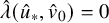 $\hat \lambda (\hat u_*,\hat v_0)=0$
and
$\hat \lambda (\hat u_*,\hat v_0)=0$
and
 $\hat \lambda \ge 0$
on
$\hat \lambda \ge 0$
on
 $[\hat u_{\mathcal H^+},\hat u_*]\times \{\hat v_0\}$
. We may then argue again using monotonicity that
$[\hat u_{\mathcal H^+},\hat u_*]\times \{\hat v_0\}$
. We may then argue again using monotonicity that
 $M\ge \varpi (\hat u_*,\hat v_0)$
and
$M\ge \varpi (\hat u_*,\hat v_0)$
and
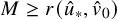 $M\ge r(\hat u_*,\hat v_0)$
. The argument in the previous paragraph now implies that
$M\ge r(\hat u_*,\hat v_0)$
. The argument in the previous paragraph now implies that
 $\varpi (\hat u_*,\hat v_0)=r(\hat u_*,\hat v_0)=M$
, which contradicts the assumption that
$\varpi (\hat u_*,\hat v_0)=r(\hat u_*,\hat v_0)=M$
, which contradicts the assumption that
 $\hat u_0>\hat u_{\mathcal H^+}$
.
$\hat u_0>\hat u_{\mathcal H^+}$
.
This completes the proof of Theorem 3.7.
9 Fine properties of the scalar field on and near the event horizon
In this section, we use the decay estimates for the geometry and the scalar field derived in the previous section to further analyze the behavior of the scalar field on and near the event horizon
 $\mathcal H^+$
of the solutions given by Theorem 3.7. In Section 9.1, we investigate the Aretakis instability on the dynamical geometry, which proves Theorem 3.9. In particular, we prove that each of the solutions given by Theorem 3.7 has an “asymptotic Aretakis charge”
$\mathcal H^+$
of the solutions given by Theorem 3.7. In Section 9.1, we investigate the Aretakis instability on the dynamical geometry, which proves Theorem 3.9. In particular, we prove that each of the solutions given by Theorem 3.7 has an “asymptotic Aretakis charge”
 $H_0[\phi ]$
, which while not actually constant, is “almost” constant in a quantitative sense. In Section 9.2, we derive sharp pointwise asymptotics for
$H_0[\phi ]$
, which while not actually constant, is “almost” constant in a quantitative sense. In Section 9.2, we derive sharp pointwise asymptotics for
 $\psi $
near
$\psi $
near
 $\mathcal H^+$
. Finally, in Section 9.3, we show that if the final Aretakis charge
$\mathcal H^+$
. Finally, in Section 9.3, we show that if the final Aretakis charge
 $H_0[\phi ]$
is “quantitatively nonvanishing,” then no nondegenerate integrated energy decay statement is true near
$H_0[\phi ]$
is “quantitatively nonvanishing,” then no nondegenerate integrated energy decay statement is true near
 $\mathcal H^+$
, which proves the sharpness of the horizon hierarchy proved in Section 6. For a discussion of these results, we refer the reader back to Section 1.4.1.
$\mathcal H^+$
, which proves the sharpness of the horizon hierarchy proved in Section 6. For a discussion of these results, we refer the reader back to Section 1.4.1.
-
In this section, we will always work with one of the solutions
$(\hat {\mathcal{Q}}_{\mathrm{max}},r,\hat \Omega ^2,\phi ,e)$
arising from seed data lying in
${\mathfrak{M}}_{\mathrm{stab}}$
. In particular, the conclusions of Theorem 3.7 hold for this solution.


9.1 Proof of the Aretakis instability, Theorem 3.9
Recall the gauge-invariant vector field
 $$ \begin{align*} Y\doteq \nu^{-1}\partial_u, \end{align*} $$
which equals
 $\partial _r$
in standard ingoing Eddington–Finkelstein coordinates
$\partial _r$
in standard ingoing Eddington–Finkelstein coordinates
 $(v,r)$
in Reissner–Nordström. For a general spherically symmetric spacetime, we derive at once the commutation formula
$(v,r)$
in Reissner–Nordström. For a general spherically symmetric spacetime, we derive at once the commutation formula
 $$ \begin{align*} [\partial_v,Y]= -\frac{\partial_u\partial_vr}{\nu}Y, \end{align*} $$
which will be useful in deriving equations for
 $\partial _v(Y\psi )$
and
$\partial _v(Y\psi )$
and
 $\partial _v(Y^2\psi )$
, where, as before,
$\partial _v(Y^2\psi )$
, where, as before,
 $\psi \doteq r\phi $
.
$\psi \doteq r\phi $
.
Lemma 9.1. Let
 $(\mathcal{Q},r,\Omega ^2,\phi ,e)$
be a solution of the spherically symmetric Einstein–Maxwell-scalar field system. Then
$(\mathcal{Q},r,\Omega ^2,\phi ,e)$
be a solution of the spherically symmetric Einstein–Maxwell-scalar field system. Then
 $$ \begin{align} \partial_v(Y\psi)+(2\kappa\varkappa) Y\psi = 2\kappa\varkappa\,\phi. \end{align} $$
Proof. Using the commutation formula and (2.17), we compute
 $$ \begin{align*} \partial_v(Y\psi)=[\partial_v,Y]\psi +Y(\partial_v\psi)=-\frac{\partial_u\partial_vr}{\nu}Y\psi + \frac{\partial_u\partial_vr}{\nu}\phi. \end{align*} $$
Lemma 9.2. Let
 $(\mathcal{Q},r,\Omega ^2,\phi ,e)$
be a solution of the spherically symmetric Einstein–Maxwell-scalar field system. Then
$(\mathcal{Q},r,\Omega ^2,\phi ,e)$
be a solution of the spherically symmetric Einstein–Maxwell-scalar field system. Then
 $$ \begin{align} \partial_v(Y^2\psi)+(4 \kappa\varkappa) Y^2\psi = -\frac{2\kappa e^2}{r^4}Y\psi+E, \end{align} $$
where
 $$ \begin{align} E\doteq \frac{2\kappa e^2}{r^3}\phi+(1-\mu)r\kappa (Y\phi)^3+2\kappa\varkappa\left(r^2(Y\phi)^3-Y\phi\right). \end{align} $$
Proof. We rewrite (9.1) as
 $$ \begin{align*} \partial_v(Y\psi)= \frac{\partial_u\partial_vr}{\nu}(\phi-Y\psi) \end{align*} $$
and apply again the commutation formula to obtain
 $$ \begin{align*} \partial_v(Y^2\psi)&= [\partial_v,Y]Y\psi + Y\partial_v(Y\psi)\\ &= -\frac{\partial_u\partial_vr}{\nu}Y^2\psi+ Y\left[\frac{\partial_u\partial_vr}{\nu}(\phi-Y\psi)\right]\\ &= -\frac{\partial_u\partial_vr}{\nu}Y^2\psi+ Y\left(\frac{\partial_u\partial_vr}{\nu}\right)(\phi-Y\psi)+ \frac{\partial_u\partial_vr}{\nu}Y(\phi-Y\psi),\\ &= -2\frac{\partial_u\partial_vr}{\nu}Y^2\psi +\frac{\partial_u\partial_vr}{\nu}Y\phi+Y\left(\frac{\partial_u\partial_vr}{\nu}\right)(\phi-Y\psi) \end{align*} $$
Using (2.18), (2.20), and (2.22), we compute
 $$ \begin{align*} Y\left(\frac{\partial_u\partial_vr}{\nu}\right)=2r\kappa\varkappa(Y\phi)^2-\frac{4\kappa\varkappa}{r}+(1-\mu)\kappa (Y\phi)^2+\frac{2\kappa e^2}{r^4}. \end{align*} $$
By grouping terms appropriately, we arrive at (9.2) and (9.3).
Proof of Theorem 3.9.
We work in one of the spacetimes
 $(\hat {\mathcal{Q}}_{\mathrm{max}},r,\hat \Omega ^2,\phi ,e)$
given by Theorem 3.7 with the initial data normalized coordinates
$(\hat {\mathcal{Q}}_{\mathrm{max}},r,\hat \Omega ^2,\phi ,e)$
given by Theorem 3.7 with the initial data normalized coordinates
 $(\hat u,\hat v)$
. Recall that the event horizon
$(\hat u,\hat v)$
. Recall that the event horizon
 $\mathcal H^+$
is located at
$\mathcal H^+$
is located at
 $\hat u=\hat u_{\mathcal H^+}$
.
$\hat u=\hat u_{\mathcal H^+}$
.
Almost-conservation of
 $Y\psi |_{\mathcal H^+}$
: We use an integrating factor to solve (9.1) on
$Y\psi |_{\mathcal H^+}$
: We use an integrating factor to solve (9.1) on
 $\mathcal H^+$
:
$\mathcal H^+$
:
 $$ \begin{align*} Y\psi(\hat u_{\mathcal H^+},\hat v_2)=\exp\left(-\int_{\hat v_1}^{\hat v_2}2\hat\kappa\varkappa\,d\hat v'\right)Y\psi(\hat u_{\mathcal H^+},\hat v_1) +\int_{\hat v_1}^{\hat v_2} \exp\left(-\int_{\hat v'}^{\hat v_2}2\hat\kappa\varkappa\, d\hat v"\right)2\hat\kappa\varkappa\,\phi\,d\hat v' \end{align*} $$
for every
 $0\le \hat v_1\le \hat v_2$
, where every quantity on the right-hand side is evaluated at
$0\le \hat v_1\le \hat v_2$
, where every quantity on the right-hand side is evaluated at
 $\hat u=\hat u_{\mathcal H^+}$
. By integrating (8.39) along
$\hat u=\hat u_{\mathcal H^+}$
. By integrating (8.39) along
 $\mathcal H^+$
and using (5.23), we find
$\mathcal H^+$
and using (5.23), we find
 $$ \begin{align*} \int_{\hat v_1}^{\hat v_2}|\hat\kappa\varkappa|_{\mathcal H^+}|\,d\hat v'\lesssim \varepsilon^{2}(1+\hat v_1)^{-1+\delta},\quad \exp\left(-\int_{\hat v_1}^{\hat v_2}2\hat\kappa\varkappa|_{\mathcal H^+}\,d\hat v'\right) = 1+O\big(\varepsilon^{2}(1+\hat v_1)^{-1+\delta}\big). \end{align*} $$
Using these, (3.21), and (3.16), we estimate
 $$ \begin{align} |Y\psi(\hat u_{\mathcal H^+},\hat v_2)-Y\psi(\hat u_{\mathcal H^+},\hat v_1)|\lesssim \varepsilon^{2}(1+\hat v_1)^{-1+\delta}|Y\psi(u_{\mathcal H^+},\hat v_1)|+ \int_{\hat v_1}^{\hat v_2}|\hat\kappa\varkappa||\phi|\,d\hat v'\lesssim \varepsilon^{3}(1+\hat v_1)^{-1+\delta}. \end{align} $$
By an elementary Cauchy sequence argument, the limit
 $$ \begin{align*} H_0[\phi]\doteq \lim_{\hat v\to\infty} Y\psi(\hat u_{\mathcal H^+},\hat v) \end{align*} $$
exists and the estimate (3.22) holds.
Proof that
 ${\mathfrak{M}}_{\mathrm{stab}}^{\ne 0}$
has nonempty interior: Let
${\mathfrak{M}}_{\mathrm{stab}}^{\ne 0}$
has nonempty interior: Let
 $\mathring \varphi $
be a compactly supported smooth function on
$\mathring \varphi $
be a compactly supported smooth function on
 $\hat {\mathcal C}$
such that
$\hat {\mathcal C}$
such that
 $$ \begin{align} \left. \frac{d}{d\hat u}\big((100M_0-\hat u)\mathring\varphi_{\mathrm{in}}\big)\right|{}_{\hat u=\hat u_{\mathcal H^+,0}}\ne 0. \end{align} $$
Let
 $0<\varepsilon \le \varepsilon _{\mathrm{stab}}$
and set
$0<\varepsilon \le \varepsilon _{\mathrm{stab}}$
and set
 $\mathcal S_0'\doteq ( c\varepsilon \mathring \varphi , 100M_0,M_0,e_0 )$
, where
$\mathcal S_0'\doteq ( c\varepsilon \mathring \varphi , 100M_0,M_0,e_0 )$
, where
 $c>0$
is a constant chosen so that
$c>0$
is a constant chosen so that
 $\mathfrak D[\mathcal S_0']\le \frac 12\varepsilon $
. In particular, c is independent of
$\mathfrak D[\mathcal S_0']\le \frac 12\varepsilon $
. In particular, c is independent of
 $\varepsilon $
. For
$\varepsilon $
. For
 $\eta>0$
small, we now set
$\eta>0$
small, we now set
 $$ \begin{align*} \mathfrak O_\eta\doteq\{\mathcal L(\mathcal S_0,\varepsilon):\mathcal S_0\in{\mathfrak{M}}_0,\mathfrak D[\mathcal S_0-\mathcal S_0']<\eta\}. \end{align*} $$
Clearly,
 $\mathfrak O_\eta $
is open in
$\mathfrak O_\eta $
is open in
 ${\mathfrak{M}}$
and we claim that for
${\mathfrak{M}}$
and we claim that for
 $\varepsilon $
and
$\varepsilon $
and
 $\eta $
sufficiently small,
$\eta $
sufficiently small,
 $\emptyset \ne \mathfrak O_\eta \cap {\mathfrak{M}}_{\mathrm{stab}}\subset {\mathfrak{M}}_{\mathrm{stab}}^{\ne 0}$
.
$\emptyset \ne \mathfrak O_\eta \cap {\mathfrak{M}}_{\mathrm{stab}}\subset {\mathfrak{M}}_{\mathrm{stab}}^{\ne 0}$
.
For
 $\eta $
small and
$\eta $
small and
 $\mathcal S_0\in \mathfrak O_\eta $
, Theorem 3.7 applies to
$\mathcal S_0\in \mathfrak O_\eta $
, Theorem 3.7 applies to
 $\mathcal L(\mathcal S_0,\varepsilon )$
. Let
$\mathcal L(\mathcal S_0,\varepsilon )$
. Let
 $\mathcal S\in {\mathfrak{M}}_{\mathrm{stab}}(\mathcal S_0,\varepsilon )$
, let
$\mathcal S\in {\mathfrak{M}}_{\mathrm{stab}}(\mathcal S_0,\varepsilon )$
, let
 $H_0[\phi ]$
be the associated asymptotic Aretakis charge. By (8.27) and (9.5), there exists a constant
$H_0[\phi ]$
be the associated asymptotic Aretakis charge. By (8.27) and (9.5), there exists a constant
 $c'>0$
such that
$c'>0$
such that
 $$\begin{align*}|Y\psi(\hat u_{\mathcal H^+},0)|\gtrsim \varepsilon - c'\eta^{1/2}\gtrsim \varepsilon\end{align*}$$
for
 $\varepsilon $
and
$\varepsilon $
and
 $\eta $
sufficiently small. By (9.4),
$\eta $
sufficiently small. By (9.4),
 $H_0[\phi ]$
differs from
$H_0[\phi ]$
differs from
 $Y\psi (\hat u_{\mathcal H^+},0)$
by an
$Y\psi (\hat u_{\mathcal H^+},0)$
by an
 $O(\varepsilon ^{3})$
quantity, and is therefore nonzero for
$O(\varepsilon ^{3})$
quantity, and is therefore nonzero for
 $\varepsilon $
sufficiently small. As this applies for every
$\varepsilon $
sufficiently small. As this applies for every
 $\mathcal S_0\in \mathfrak O_\eta $
, we have proved that
$\mathcal S_0\in \mathfrak O_\eta $
, we have proved that
 $\emptyset \ne \mathfrak O_\eta \cap {\mathfrak{M}}_{\mathrm{stab}}\subset {\mathfrak{M}}_{\mathrm{stab}}^{\ne 0}$
, which shows that
$\emptyset \ne \mathfrak O_\eta \cap {\mathfrak{M}}_{\mathrm{stab}}\subset {\mathfrak{M}}_{\mathrm{stab}}^{\ne 0}$
, which shows that
 ${\mathfrak{M}}_{\mathrm{stab}}^{\ne 0}$
has nonempty interior in the subspace topology.
${\mathfrak{M}}_{\mathrm{stab}}^{\ne 0}$
has nonempty interior in the subspace topology.
Linear growth of
 $Y^2\psi |_{\mathcal H^+}$
: We use an integrating factor to solve (9.2) on
$Y^2\psi |_{\mathcal H^+}$
: We use an integrating factor to solve (9.2) on
 $\mathcal H^+$
:
$\mathcal H^+$
:
 $$ \begin{align*} Y^2\psi(\hat u_{\mathcal H^+},\hat v)=\exp\left(-\int_{0}^{\hat v}4\hat\kappa\varkappa\,d\hat v'\right)Y^2\psi(\hat u_{\mathcal H^+},0) +\int_{0}^{\hat v} \exp\left(-\int_{\hat v'}^{\hat v_2}4\hat\kappa\varkappa\,d\hat v"\right)\left(-\frac{2\hat\kappa e^2}{r^4}Y\psi+E\right)d\hat v'. \end{align*} $$
The first term is
 $O(\varepsilon )$
by our assumption on the initial data (recall (3.24)) and by (8.38), (8.39), (3.21), and (3.16), we have
$O(\varepsilon )$
by our assumption on the initial data (recall (3.24)) and by (8.38), (8.39), (3.21), and (3.16), we have
 $$ \begin{align*} \big|E|_{\mathcal H^+}\big|\lesssim \varepsilon\tau^{-1+\delta/2}. \end{align*} $$
Note that the worst decaying term in E (by far) comes from the zeroth order term, for which we only have the nonintegrable decay estimate (3.21). Using again the geometric estimates on the horizon and (9.4), we have
 $$ \begin{align*} \int_0^{\hat v}\frac{2\hat\kappa e^2}{r^4}Y\psi\,d\hat v'=\int_0^{\mathfrak v(\hat v)}\frac{2\kappa e^2}{r^4}Y\psi\,dv'= \frac{2}{M^2}H_0[\phi]\hat v + O\big(\varepsilon^{3}(1+\hat v)^\delta\big). \end{align*} $$
Putting these estimates together, we have
 $$ \begin{align*} \left|Y^2\psi(\hat u_{\mathcal H^+},\hat v)+\frac{2}{M^2}H_0[\phi]\hat v\right| \lesssim \varepsilon(1+\hat v)^{\delta/2}+\varepsilon^{3}(1+\hat v)^\delta, \end{align*} $$
which implies (3.25).
Behavior of the Ricci tensor along
 $\mathcal H^+$
: By trace-reversing the Einstein equation, we find
$\mathcal H^+$
: By trace-reversing the Einstein equation, we find
 $$ \begin{align*} R_{\mu\nu}= 2T_{\mu\nu}^{\mathrm{EM}}+2\partial_\mu\phi\partial_\nu\phi \end{align*} $$
and using (2.3) we compute
 $$ \begin{align*} T^{\mathrm{EM}}= \frac{\hat\Omega^2e^2}{4r^4}(d\hat u\otimes d\hat v+d\hat v\otimes d\hat u)+\frac{e^2}{2r^2}g_{S^2}.\end{align*} $$
Therefore,
 $$ \begin{align*} R_{\mu\nu}Y^\mu Y^\nu = 2(Y\phi)^2 = 2r^{-2}(Y\psi)^2-4r^{-3}\psi Y\psi +2r^{-4}\psi^2, \end{align*} $$
from which (3.23) follows readily.
Next, we compute
 $$ \begin{align*} \nabla_\rho R_{\mu\nu} = 2\nabla_\rho T_{\mu\nu}^{\mathrm{EM}}+2\nabla_\rho\nabla_\mu\phi\nabla_\nu\phi+2\nabla_\mu\phi\nabla_\rho\nabla_\nu\phi. \end{align*} $$
Using again the form of
 $T^{\mathrm{EM}}$
, we have
$T^{\mathrm{EM}}$
, we have
 $\nabla _\rho T_{\mu \nu }^{\mathrm{EM}}Y^\rho Y^\mu Y^\nu =0$
. Since
$\nabla _\rho T_{\mu \nu }^{\mathrm{EM}}Y^\rho Y^\mu Y^\nu =0$
. Since
 $$\begin{align*}\Gamma^{\hat u}_{\hat u\hat u}=\partial_{\hat u}{\log\hat\Omega^2}=\partial_{\hat u}{\log(-4\hat\kappa\hat\nu)}=\hat\kappa^{-1}\partial_{\hat u}\hat\kappa+\hat\nu^{-1}\partial_{\hat u}\hat\nu,\end{align*}$$
it holds that
 $$ \begin{align*} \nabla_\rho\nabla_\mu\phi \,Y^\rho Y^\mu& = \hat \nu^{-2} \partial_{\hat u}^2\phi -\hat\nu^{-2}\big(\hat\kappa^{-1}\partial_{\hat u}\hat\kappa+\hat\nu^{-1}\partial_{\hat u}\hat\nu\big)\partial_{\hat u}\phi\\ &=\hat\nu^{-2}\partial_{\hat u}(\hat\nu Y\phi) - \hat\nu^{-1}\big(r\hat\nu (Y\phi)^2+\hat\nu^{-1}\partial_{\hat u}\hat\nu\big) Y\phi\\ &= Y^2\phi -r(Y\phi)^3 \end{align*} $$
and hence
 $$ \begin{align*} \nabla_\rho R_{\mu\nu} Y^\rho Y^\mu Y^\nu = 4 Y\phi Y^2\phi - 4r(Y\phi)^4, \end{align*} $$
from which (3.26) follows readily.
9.2 Sharp decay for the scalar field near the horizon
In this section, we work in the eschatological gauge
 $(u_\infty ,v)$
on the domain
$(u_\infty ,v)$
on the domain
 $\mathcal D_\infty $
with the final anchored extremal Reissner–Nordström solution
$\mathcal D_\infty $
with the final anchored extremal Reissner–Nordström solution
 $\bar r_\infty $
.
$\bar r_\infty $
.
We require the following lemma (see also (2.26)).
Lemma 9.3. On
 $\mathcal D_\infty \cap \{\bar r_\infty \le \tfrac 12\Lambda \}$
, it holds that
$\mathcal D_\infty \cap \{\bar r_\infty \le \tfrac 12\Lambda \}$
, it holds that
 $$ \begin{align} \frac{1}{\bar r_\infty-M}\sim u_\infty-v. \end{align} $$
Proof. We have the identity
 $$ \begin{align} v-u_\infty = \int_{\bar r_\star}^{\bar r_\infty}\frac{d\bar r'}{D(\bar r')}= -\frac{M^2}{\bar r_\infty-M}+\frac{M^2}{\bar r_\star-M}+2M\log\left(\frac{\bar r_\infty-M}{\bar r_\star-M}\right)+\bar r_\infty-\bar r_\star \end{align} $$
on
 $\mathcal D_\infty $
, where
$\mathcal D_\infty $
, where
 $\bar r_\star $
was defined in (8.18) and
$\bar r_\star $
was defined in (8.18) and
 $D(r)\doteq (1-M/r)^2$
. Indeed, this is trivially true at the bifurcation sphere
$D(r)\doteq (1-M/r)^2$
. Indeed, this is trivially true at the bifurcation sphere
 $(u_\infty ,v)=(0,0)$
by definition of
$(u_\infty ,v)=(0,0)$
by definition of
 $\bar r_\star $
, and holds everywhere because the
$\bar r_\star $
, and holds everywhere because the
 $\partial _{u_\infty }$
and
$\partial _{u_\infty }$
and
 $\partial _v$
derivatives of
$\partial _v$
derivatives of
 $v-u_\infty $
and the integral are equal. Writing (9.7) as
$v-u_\infty $
and the integral are equal. Writing (9.7) as
 $$ \begin{align} u_\infty-v = \frac{M^2}{\bar r_\infty-M} - 2M\log(\bar r_\infty-M) +O(1), \end{align} $$
we infer (9.6) by inspection.
Let us consider the curve
 $$ \begin{align} \mathcal{\sigma}_{\beta} \doteq \{(u_\infty,v)\in\mathcal D_\infty: u_\infty -v = u_{\infty}^{\beta} + C_\beta \}, \end{align} $$
where the constant
 $C_\beta $
is chosen so that
$C_\beta $
is chosen so that
 $\sigma _\beta \subset \{\bar r_\infty \le \frac 12\Lambda \}$
. We also define the spacetime region
$\sigma _\beta \subset \{\bar r_\infty \le \frac 12\Lambda \}$
. We also define the spacetime region
 $$ \begin{align} \mathfrak{t}_{\beta} \doteq \{(u_\infty,v)\in\mathcal D_\infty: v \leq u_{\infty}-u_{\infty}^{\beta} - C_\beta \}. \end{align} $$
Using (9.6), we observe that in the region
 $\mathfrak{t}_{\beta }$
,
$\mathfrak{t}_{\beta }$
,
 $$ \begin{align} \bar{r}_{\infty} - M \lesssim (1+u_{\infty})^{-\beta} \lesssim (1+v)^{-\beta}. \end{align} $$
With these definitions, we have the following result:
Proposition 9.4. Under the assumption (3.24), for every
 $\beta \in (\frac 23,1)$
, there exists a
$\beta \in (\frac 23,1)$
, there exists a
 $\beta '>0$
such that
$\beta '>0$
such that
 $$ \begin{align} | u_{\infty}^2 \partial_{u_{\infty}} \psi + M^2 H_0 [ \phi ] | \lesssim \varepsilon^{3} +\varepsilon u_{\infty}^{-\beta'} \end{align} $$
in
 $\mathfrak t_\beta $
, where
$\mathfrak t_\beta $
, where
 $H_0[\phi ]$
is the asymptotic Aretakis charge of the wave.
$H_0[\phi ]$
is the asymptotic Aretakis charge of the wave.
We first verify the proposition along
 $\underline C{}_{\mathrm{in}}$
.
$\underline C{}_{\mathrm{in}}$
.
Lemma 9.5. Let
 $\eta>0$
. Under the assumption (3.24), it holds that
$\eta>0$
. Under the assumption (3.24), it holds that
 $$ \begin{align} |u^2_\infty\partial_{u_\infty}\psi(u_\infty,0)+M^2H_0[\phi]|\lesssim \varepsilon^3+\varepsilon u_\infty^{-1+\eta} \end{align} $$
for all
 $u_\infty>0$
.
$u_\infty>0$
.
Proof. Using the chain rule and (8.33), we estimate
 $$ \begin{align*} \partial_{\hat u}\big((\bar r_\infty-M)\circ\Phi_\infty(\hat u,0)\big) = \bar\nu_\infty\big(\Phi_\infty(\hat u,0)\big) \partial_{\hat u}\Phi(\hat u,0)\sim \nu_\infty\big(\Phi_\infty(\hat u,0)\big) \partial_{\hat u}\Phi(\hat u,0)=\hat\nu(\hat u,0)=-1. \end{align*} $$
Therefore, integrating backwards from
 $\hat u_{\mathcal H^+}$
, we find that
$\hat u_{\mathcal H^+}$
, we find that
 $$ \begin{align*} (\bar r_\infty-M)\circ\Phi_\infty(\hat u,0)\sim \hat u_{\mathcal H^+}-\hat u \end{align*} $$
for
 $\hat u\in [0,\hat u_{\mathcal H^+}]$
. By Taylor’s theorem, the estimate (9.4), and the assumption (3.24), we have that
$\hat u\in [0,\hat u_{\mathcal H^+}]$
. By Taylor’s theorem, the estimate (9.4), and the assumption (3.24), we have that
 $$ \begin{align*} Y\psi(\hat u,0)= H_0[\phi] + O\big(\varepsilon(\bar r_\infty-M)\big)+O(\varepsilon^3) \end{align*} $$
for
 $\hat u\in [0,\hat u_{\mathcal H^+}]$
. Of course,
$\hat u\in [0,\hat u_{\mathcal H^+}]$
. Of course,
 $H_0[\phi ]=O(\varepsilon )$
as well.
$H_0[\phi ]=O(\varepsilon )$
as well.
By (9.8), the identity
 $\bar \nu _\infty = -\bar r_\infty ^{-2}(\bar r_\infty -M)^2$
, and the Taylor expansion
$\bar \nu _\infty = -\bar r_\infty ^{-2}(\bar r_\infty -M)^2$
, and the Taylor expansion
 $\bar r^{-2}_\infty = M^{-2}+O(\bar r_\infty -M)$
, we have
$\bar r^{-2}_\infty = M^{-2}+O(\bar r_\infty -M)$
, we have
 $$ \begin{align*} u^2_\infty \bar \nu_\infty = -M^2+O\big((\bar r_\infty-M)[1+\log(\bar r_\infty-M)]\big) \end{align*} $$
at
 $v=0$
, and we may therefore compute
$v=0$
, and we may therefore compute
 $$ \begin{align*} u^2_\infty\partial_{u_\infty}\psi = u^2_\infty \nu_\infty Y\psi =u_\infty^2\bar\nu_\infty\big(1+O(\varepsilon^3)\big)Y\psi =-M^2H_0[\phi] +O\big(\varepsilon(\bar r_\infty-M)[1+\log(\bar r_\infty-M)]\big)+O(\varepsilon^3) \end{align*} $$
at
 $v=0$
. Using the estimate
$v=0$
. Using the estimate
 $x\log x\lesssim x^{1-\eta }$
, we arrive at (9.13).
$x\log x\lesssim x^{1-\eta }$
, we arrive at (9.13).
Proof of Proposition 9.4.
Integrating the wave equation (2.19) along the segment
 $\{u_\infty \}\times [0,v]\subset \mathfrak t_\beta $
, we have
$\{u_\infty \}\times [0,v]\subset \mathfrak t_\beta $
, we have
 $$ \begin{align*}u_{\infty}^2 \partial_{u_{\infty}} \psi ( u_{\infty} , v ) = u_{\infty}^2 \partial_{u_{\infty}} \psi ( u_{\infty} , 0 ) + u_{\infty}^2 \int_0^v \frac{2\kappa_\infty\nu_\infty\varkappa}{r} \psi \, dv' .\end{align*} $$
By (5.7), (5.41), (5.32), and (8.36), (8.33), (8.39), the second term on the right-hand side satisfies
 $$ \begin{align} &\left| u_{\infty}^2 \int_0^v \frac{2\kappa_\infty\nu_\infty\varkappa}{r} \psi \, dv'\right| \lesssim u_{\infty}^2 \int_0^v ( \bar{r}_{\infty} - M)^3 | \psi | \, dv' + u_{\infty}^2 \int_0^v \varepsilon^2 (1+v')^{-2+\delta}( \bar{r}_{\infty} - M )^2 | \psi | \, dv' \nonumber \\& \quad \lesssim u_{\infty}^{-\beta'} \int_0^v u_{\infty}^{2+\beta'} ( \bar{r}_{\infty} - M)^3 | \psi | \, dv' + \int_0^v \varepsilon^{2} u_{\infty}^2 (1+v')^{-2+\delta}( \bar{r}_{\infty} - M )^2| \psi | \, dv'. \end{align} $$
For the first term of the last expression we note that by (3.21) and (9.11), we have
 $$ \begin{align*} u_{\infty}^{-\beta'} \int_0^v u_{\infty}^{2+\beta'} ( \bar{r}_{\infty} - M)^3 | \psi | \, dv' \lesssim \varepsilon u_{\infty}^{-\beta'} \int_0^v (1+v' )^{-1+\delta/2 -3\beta + 2 + \beta' } dv' \lesssim \varepsilon u_{\infty}^{-\beta'} , \end{align*} $$
as
 $-1+\delta /2 - 3 \beta + 2 + \beta ' < -1$
for
$-1+\delta /2 - 3 \beta + 2 + \beta ' < -1$
for
 $\beta \in (2/3 , 1)$
and
$\beta \in (2/3 , 1)$
and
 $\beta '> 0$
sufficiently small.
$\beta '> 0$
sufficiently small.
To handle the second term on the right-hand side of (9.14), we break the region
 $\mathfrak{t}_{\beta }$
into two pieces. We split
$\mathfrak{t}_{\beta }$
into two pieces. We split
 $\mathfrak t_\beta $
along the curve
$\mathfrak t_\beta $
along the curve
 $$\begin{align*}\rho_\beta\doteq \{(u_\infty,v)\in\mathcal D_\infty:v= \tfrac 12 u_\infty-C_\beta'\},\end{align*}$$
where
 $C_\beta '$
is chosen so that
$C_\beta '$
is chosen so that
 $\rho _\beta \cap \sigma _\beta =\emptyset $
. Denote the region between
$\rho _\beta \cap \sigma _\beta =\emptyset $
. Denote the region between
 $\rho _\beta $
and
$\rho _\beta $
and
 $\mathcal H^+$
by
$\mathcal H^+$
by
 $\mathfrak t^1_\beta $
and the region between
$\mathfrak t^1_\beta $
and the region between
 $\rho _\beta $
and
$\rho _\beta $
and
 $\sigma _\beta $
by
$\sigma _\beta $
by
 $\mathfrak t^2_\beta $
, so that
$\mathfrak t^2_\beta $
, so that
 $\mathfrak t_\beta =\mathfrak t^1_\beta \cup \mathfrak t^2_\beta $
. In
$\mathfrak t_\beta =\mathfrak t^1_\beta \cup \mathfrak t^2_\beta $
. In
 $\mathfrak{t}^1_{\beta }$
, it holds that
$\mathfrak{t}^1_{\beta }$
, it holds that
 $\bar {r}_{\infty }-M \lesssim (1+u_{\infty })^{-1}$
, which implies that
$\bar {r}_{\infty }-M \lesssim (1+u_{\infty })^{-1}$
, which implies that
 $$ \begin{align*} \int_0^v \varepsilon^{2} u_{\infty}^2 (1+v')^{-2+\delta}( \bar{r}_{\infty} - M )^2| \psi |\mathbf{1}_{\mathfrak t_\beta^1} \, dv' \lesssim \varepsilon^3. \end{align*} $$
On the other hand, in
 $\mathfrak{t}^2_{\beta }$
, it holds that
$\mathfrak{t}^2_{\beta }$
, it holds that
 $(1+v)^{-1}\lesssim (1+ u_{\infty })^{-1}$
, so using (9.11) we estimate
$(1+v)^{-1}\lesssim (1+ u_{\infty })^{-1}$
, so using (9.11) we estimate
 $$ \begin{align*} \int_0^v \varepsilon^{2} u_{\infty}^2 (1+v')^{-2+\delta}( \bar{r}_{\infty} - M )^2| \psi |\mathbf{1}_{\mathfrak t_\beta^2} \, dv'\lesssim \varepsilon^2u_\infty^{2-k-2\beta}\int_0^v(1+v')^{-3+k+3\delta/2} \,dv'\lesssim \varepsilon^3u_\infty^{-\beta'} \end{align*} $$
where k is chosen so that
 $-2+k+2\beta>\beta '$
and
$-2+k+2\beta>\beta '$
and
 $-3+k+3\delta /2<-1$
.
$-3+k+3\delta /2<-1$
.
By applying Lemma 9.5 with
 $\eta $
chosen such that
$\eta $
chosen such that
 $-1+\eta <\beta '$
, we conclude (9.12).
$-1+\eta <\beta '$
, we conclude (9.12).
We now use the previous proposition to obtain improved decay for
 $\psi $
in
$\psi $
in
 $\mathfrak{t}_{\beta }$
.
$\mathfrak{t}_{\beta }$
.
Proposition 9.6. Under the assumptions of Proposition 9.4 and
 $\beta \in (\frac 23,1-\delta -2\beta ')$
, it holds that
$\beta \in (\frac 23,1-\delta -2\beta ')$
, it holds that
 $$ \begin{align} \left| \psi ( u_{\infty} , v ) + M^2 H_0 [ \phi ] \left(v^{-1} - u_\infty^{-1} \right) \right| \lesssim \varepsilon^3|v^{-1} - u_\infty^{-1} |+\varepsilon (1+v)^{-1-\beta'} \end{align} $$
in
 $\mathfrak t_\beta $
.
$\mathfrak t_\beta $
.
Proof. Let
 $u_\beta =u_\beta (v)$
be defined by
$u_\beta =u_\beta (v)$
be defined by
 $(u_\beta ,v)\in \sigma _\beta $
. Then
$(u_\beta ,v)\in \sigma _\beta $
. Then
 $$ \begin{align} |\psi(u_\beta,v)|=(\bar r_\infty-M)^{-1/2}(u_\beta,v)|(\bar r_\infty-M)^{1/2}\psi|(u_\beta,v)\lesssim \varepsilon (1+v)^{-3/2+\delta/2+\beta/2}\lesssim \varepsilon(1+v)^{-1-\beta'} \end{align} $$
by (3.21), the fact that
 $(\bar r_\infty -M)^{-1}\sim 1+v$
along
$(\bar r_\infty -M)^{-1}\sim 1+v$
along
 $\sigma _\beta $
, and the assumption on
$\sigma _\beta $
, and the assumption on
 $\beta $
. Using (9.12), we find for
$\beta $
. Using (9.12), we find for
 $(u_\infty ,v)\in \mathfrak t_\beta $
,
$(u_\infty ,v)\in \mathfrak t_\beta $
,
 $$ \begin{align*} \psi (u_{\infty} , v)-\psi (u_\beta , v) &=\int_{u_\beta}^{u_\infty}\partial_{u_\infty}\psi\,du_\infty'\\&=-M^2H_0[\phi](u_\beta^{-1}-u_\infty^{-1})+O\big(\varepsilon^3(u_\beta^{-1}-u_\infty^{-1})+\varepsilon(u_\beta^{-1-\beta'}-u_\infty^{-1-\beta'})\big). \end{align*} $$
Now we note that
 $$ \begin{align*} u_\beta^{-1}-u_\infty^{-1}=(u_\beta^{-1}-v^{-1})+(v^{-1}-u_\infty^{-1})= (v^{-1}-u_\infty^{-1})+O(v^{-2+\beta}) \end{align*} $$
and
 $u_\beta +1\sim v+1$
, and (9.15) readily follows.
$u_\beta +1\sim v+1$
, and (9.15) readily follows.
9.3 Sharpness of the horizon hierarchy
We will show that the range of p in the horizon hierarchy of Section 6.3 is sharp, resulting in failure of boundedness of the integrated nondegenerate energy near the horizon.
Proposition 9.7. For any
 $\eta>0$
and
$\eta>0$
and
 $C_2>0$
there exists a constant
$C_2>0$
there exists a constant
 $0<\varepsilon _{\eta ,C_2}\le \varepsilon _{\mathrm{stab}}$
such that the following holds. Let
$0<\varepsilon _{\eta ,C_2}\le \varepsilon _{\mathrm{stab}}$
such that the following holds. Let
 $\mathcal S_0(\alpha _\star )\in {\mathfrak{M}}_{\mathrm{stab}}$
with
$\mathcal S_0(\alpha _\star )\in {\mathfrak{M}}_{\mathrm{stab}}$
with
 $0< \mathfrak D[\mathcal S_0]\le \varepsilon \le \varepsilon _{\eta ,C_2}$
. Suppose also that
$0< \mathfrak D[\mathcal S_0]\le \varepsilon \le \varepsilon _{\eta ,C_2}$
. Suppose also that
 $\mathring \phi $
satisfies the second order smallness condition (3.24) and that the asymptotic Aretakis charge is quantitatively nonvanishing in the sense that
$\mathring \phi $
satisfies the second order smallness condition (3.24) and that the asymptotic Aretakis charge is quantitatively nonvanishing in the sense that
 $$ \begin{align} |H_0[\phi]|\ge\varepsilon^{2-\eta}. \end{align} $$
Then for any
 $R> M$
, it holds that
$R> M$
, it holds that
 $$ \begin{align} \iint_{\mathcal D_\infty\cap\{\bar r_\infty\le R\} }\frac{(\partial_{u_{\infty}} \psi)^2}{-\bar{\nu}_{\infty}} \,du_\infty dv = \infty. \end{align} $$
Remark 9.8. Note that by the Morawetz estimate Proposition 6.4, the integral in (9.18), taken instead over
 $\mathcal D_\infty \cap \{R'\le \bar r_\infty \le R\}$
where
$\mathcal D_\infty \cap \{R'\le \bar r_\infty \le R\}$
where
 $M<R'<R$
, is finite.
$M<R'<R$
, is finite.
Proof of Proposition 9.7.
We repeat the main calculation for the horizon hierarchy, Lemma 6.18, with
 $p=3$
. Let
$p=3$
. Let
 $$ \begin{align*} \mathcal A_{u_f}\doteq \mathcal D_\infty\cap \{r\le\Lambda\}\cap\{u_\infty\le u_f\}, \end{align*} $$
where we will let
 $u_f\to \infty $
and
$u_f\to \infty $
and
 $v_0$
will be chosen later.
$v_0$
will be chosen later.
Integrating the expression
 $$ \begin{align*} \iint_{ \mathcal A_{u_f}} \partial_v\left((\bar r-M)^{-1}\frac{(\partial_{u_\infty}\psi)^2}{-\bar\nu_\infty}\right) du_\infty dv \end{align*} $$
by parts and using the wave equation (2.19), we find that
 $$ \begin{align} & - \int_{\underline C{}_{0}\cap \mathcal A_{u_f}} (\bar r_\infty-M)^{-1} \frac{(\partial_{u_\infty}\psi)^2}{-\bar\nu_\infty}\,du_\infty +\int_{\Gamma \cap \mathcal A_{u_f}}n^v_\Gamma (\bar r_\infty-M)^{-1}\frac{(\partial_{u_\infty}\psi)^2}{-\bar\nu_\infty}\,ds \nonumber\\ & \quad =-\iint_{\mathcal A_{u_f}}\left(\frac{2M+\bar r_\infty}{\bar r_\infty^3}\right)\frac{(\partial_{u_\infty}\psi)^2}{-\bar\nu_\infty}\,du_\infty dv -\iint_{\mathcal A_{u_f}}\frac{4\kappa_\infty \nu_\infty}{r\bar \nu_\infty}(\bar r_\infty-M)^{-1}\varkappa\psi\partial_{u_\infty}\psi\,du_\infty dv. \end{align} $$
The term along
 $\Gamma $
is
$\Gamma $
is
 $\lesssim \varepsilon ^2$
using (6.27) and (6.30). For
$\lesssim \varepsilon ^2$
using (6.27) and (6.30). For
 $\varepsilon $
sufficiently small using (9.13) with
$\varepsilon $
sufficiently small using (9.13) with
 $\eta =1-\beta '$
and the condition (9.17), we have
$\eta =1-\beta '$
and the condition (9.17), we have
 $$ \begin{align*} \big(u^2_\infty \partial_{u_\infty}\psi(u_\infty,0)\big)^2\gtrsim |H_0[\phi]|^2 -O(\varepsilon^2u_\infty^{-\beta'}) \end{align*} $$
Therefore, by (9.6), it holds that
 $$ \begin{align} & \int_{\underline C{}_{0}\cap \mathcal A_{u_f}} (\bar r_\infty-M)^{-1} \frac{(\partial_{u_\infty}\psi)^2}{-\bar\nu_\infty}\,du_\infty \gtrsim \int_{\underline C{}_{0}\cap \mathcal A_{u_f}} (\bar r_\infty-M)^{-3} (\partial_{u_\infty}\psi)^2\,du_\infty \gtrsim \int_{\underline C{}_{0}\cap \mathcal A_{u_f}}u_\infty^3 (\partial_{u_\infty}\psi)^2\,du_\infty \nonumber\\ &\qquad\qquad\quad \gtrsim\int_{\underline C{}_{0}\cap \mathcal A_{u_f}}u_\infty^{-1}\big(|H_0[\phi]|^2-O(\varepsilon^2 u_\infty^{-\beta'})\big)\,du_\infty\gtrsim |H_0[\phi]|^2\log(u_f)-\varepsilon^2, \end{align} $$
where we have used that
 $u_\infty ^{-1-\beta '}$
is integrable.
$u_\infty ^{-1-\beta '}$
is integrable.
We now estimate the mixed term on the right-hand side of (9.19). We use the geometric estimate (8.39) and break up the region of integration using
 $\mathfrak t_\beta $
to estimate
$\mathfrak t_\beta $
to estimate
 $$ \begin{align} & \left| \iint_{\mathcal A_{u_f}}\frac{4\kappa_\infty \nu_\infty}{r\bar \nu_\infty}(\bar r_\infty-M)^{-1}\varkappa\psi\partial_{u_\infty}\psi\,du_\infty dv\right|\lesssim \iint_{\mathcal A_{u_f}}|\psi||\partial_{u_\infty}\psi|\,du_\infty dv \nonumber \\& \qquad\qquad\qquad +\left(\iint_{\mathcal A_{u_f}\setminus \mathfrak t_\beta}+\iint_{\mathcal A_{u_f}\cap \mathfrak t_\beta}\right)\varepsilon^2(\bar r_\infty-M)^{-1}\tau^{-2+\delta}|\psi||\partial_{u_\infty}\psi|\,du_\infty dv \doteq \mathrm{I}+\mathrm{II}+\mathrm{III}. \end{align} $$
By (9.6), we have
 $(\bar r_\infty -M)^{-1}\lesssim u-v\le u$
in
$(\bar r_\infty -M)^{-1}\lesssim u-v\le u$
in
 $\mathcal A_{u_f}\cap \{\bar r_\infty \le \tfrac 12\Lambda \}$
and by definition of
$\mathcal A_{u_f}\cap \{\bar r_\infty \le \tfrac 12\Lambda \}$
and by definition of
 $\sigma _\beta $
,
$\sigma _\beta $
,
 $(\bar r_\infty -M)^{-1}\lesssim 1+v$
in
$(\bar r_\infty -M)^{-1}\lesssim 1+v$
in
 $\mathcal A_{u_f}\setminus \mathfrak t_\beta $
. It follows that
$\mathcal A_{u_f}\setminus \mathfrak t_\beta $
. It follows that
 $\mathrm{II}\lesssim \varepsilon ^2\mathrm{I}$
. Using the bulk terms in the energy estimate Proposition 6.14 with
$\mathrm{II}\lesssim \varepsilon ^2\mathrm{I}$
. Using the bulk terms in the energy estimate Proposition 6.14 with
 $p=5/2$
(after passing to
$p=5/2$
(after passing to
 $\tau _f\to \infty $
, refer also to the proof of Theorem 3.7 in Section 8.3.5), we have
$\tau _f\to \infty $
, refer also to the proof of Theorem 3.7 in Section 8.3.5), we have
 $\mathrm{I}\lesssim \underline {\mathcal E}^\infty _{5/2}(1)\lesssim \varepsilon ^2$
. By Proposition 9.6, we have
$\mathrm{I}\lesssim \underline {\mathcal E}^\infty _{5/2}(1)\lesssim \varepsilon ^2$
. By Proposition 9.6, we have
 $|\psi | \lesssim \varepsilon u^{-1}_\infty +\varepsilon v^{-1}$
in
$|\psi | \lesssim \varepsilon u^{-1}_\infty +\varepsilon v^{-1}$
in
 $\mathfrak t_\beta $
and by Proposition 9.4, we have
$\mathfrak t_\beta $
and by Proposition 9.4, we have
 $|u_\infty ^2\partial _{u_\infty }\psi |\lesssim \varepsilon $
in
$|u_\infty ^2\partial _{u_\infty }\psi |\lesssim \varepsilon $
in
 $\mathfrak t_\beta $
. Therefore, we estimate
$\mathfrak t_\beta $
. Therefore, we estimate
 $$ \begin{align} & \mathrm{III}\lesssim \iint_{\mathcal A_{u_f}\cap \mathfrak t^1_\beta}\varepsilon^2u_\infty^{-1}v^{-2+\delta}|\psi||u_\infty^2\partial_{u_\infty}\psi|\,du_\infty dv \nonumber\\& \qquad\qquad\quad\lesssim \varepsilon^4 + \varepsilon^4\iint_{\{1\le u_\infty\le u_f\}\cap\{v\ge 1\}} \big(u_\infty^{-2}v^{-2+\delta}+u_\infty^{-1}v^{-3+\delta}\big) du_\infty dv\lesssim \varepsilon^4(1+\log(u_f)). \end{align} $$
Combining (9.19), (9.20), (9.21), and (9.22), we find
 $$ \begin{align*} \iint_{\mathcal A_{u_f}}\frac{(\partial_{u_\infty}\psi)^2}{-\bar\nu_\infty}\,du_\infty dv\gtrsim \big(|H_0[\phi]|^2-\varepsilon^4\big)\log(u_f)-\varepsilon^2\gtrsim |H_0[\phi]|^2\log(u_f)-\varepsilon^2 \end{align*} $$
for
 $\varepsilon $
sufficiently small. Letting
$\varepsilon $
sufficiently small. Letting
 $u_f\to \infty $
completes the proof.
$u_f\to \infty $
completes the proof.
Remark 9.9. There is an interesting difference between the proof of Proposition 9.7 and the corresponding fact in the uncoupled case. In our case, the mixed bulk term on the right-hand side of (9.19) is in general not bounded as
 $u_f\to \infty $
, while it is bounded in the uncoupled case. This is because the dynamical redshift factor
$u_f\to \infty $
, while it is bounded in the uncoupled case. This is because the dynamical redshift factor
 $\varkappa $
does not in general exactly cancel out the singular factor of
$\varkappa $
does not in general exactly cancel out the singular factor of
 $(\bar r_\infty -M)^{-1}$
. Though the growth rate is logarithmic, just as with the first term on the left-hand side of (9.19), it comes with an additional smallness factor which allows the proof to go through. The cost is that we can only prove Proposition 9.7 under the “quantitative nonvanishing” assumption (9.17) on the asymptotic Aretakis charge
$(\bar r_\infty -M)^{-1}$
. Though the growth rate is logarithmic, just as with the first term on the left-hand side of (9.19), it comes with an additional smallness factor which allows the proof to go through. The cost is that we can only prove Proposition 9.7 under the “quantitative nonvanishing” assumption (9.17) on the asymptotic Aretakis charge
 $H_0[\phi ]$
. In the uncoupled case, where
$H_0[\phi ]$
. In the uncoupled case, where
 $H_0[\phi ]$
is constant, it suffices to assume that
$H_0[\phi ]$
is constant, it suffices to assume that
 $H_0[\phi ]\ne 0$
.
$H_0[\phi ]\ne 0$
.
On the other hand, in the uncoupled case on a subextremal Reissner–Nordström background, the same bulk term is also infinite. It should be noted though, in the uncoupled subextremal case, that it is infinite in a way that cancels out the other unbounded term in (9.19) (the first term on the left-hand side). As a result, in the uncoupled subextremal case, there is no contradiction with the fact that the spacetime integral (9.18) is finite due to the redshift effect [Reference Dafermos and Rodnianski30]. See [Reference Angelopoulos, Aretakis and Gajic2, Section 4.6] for more details.
Acknowledgements
The authors would like to thank Mihalis Dafermos for insightful conversations on teleology and dyadicism. They would also like to thank John Anderson, Jonathan Luk, Harvey Reall, Igor Rodnianski, Rita Teixeira da Costa, and Claude Warnick for their interest, helpful discussions, and comments.
Competing interests
The authors have no competing interests to declare.
Funding statement
R.U. acknowledges support from the NSF grant DMS-2401966 and a Miller Fellowship.


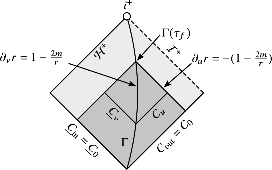


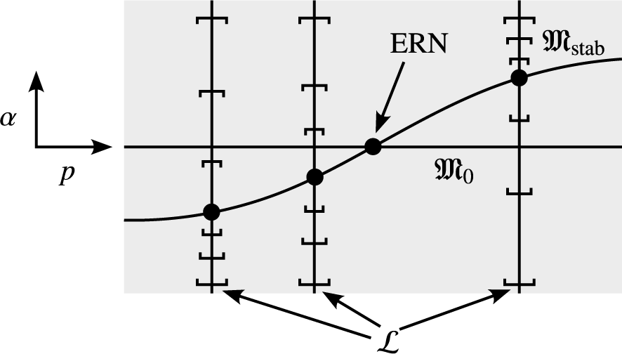


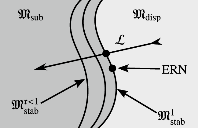


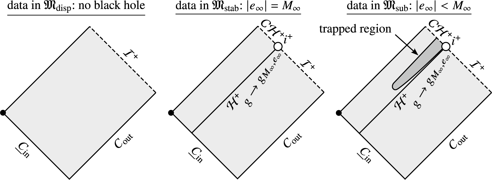


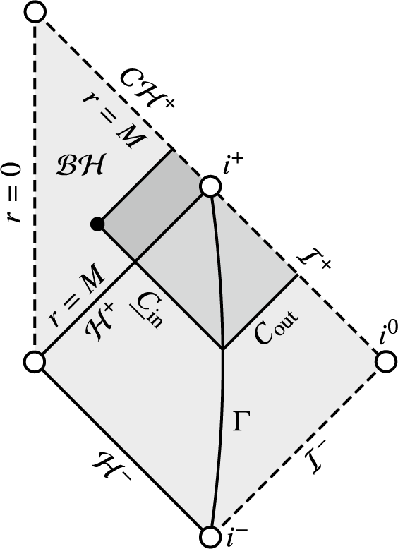

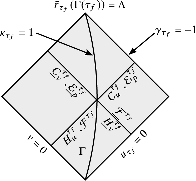


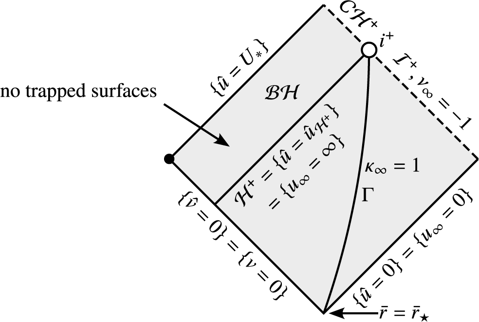

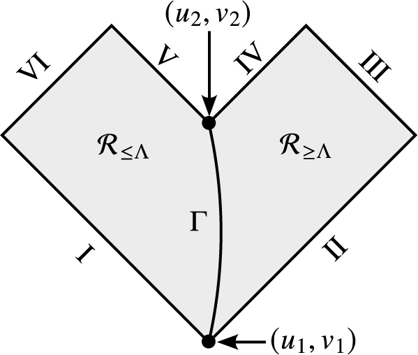

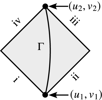
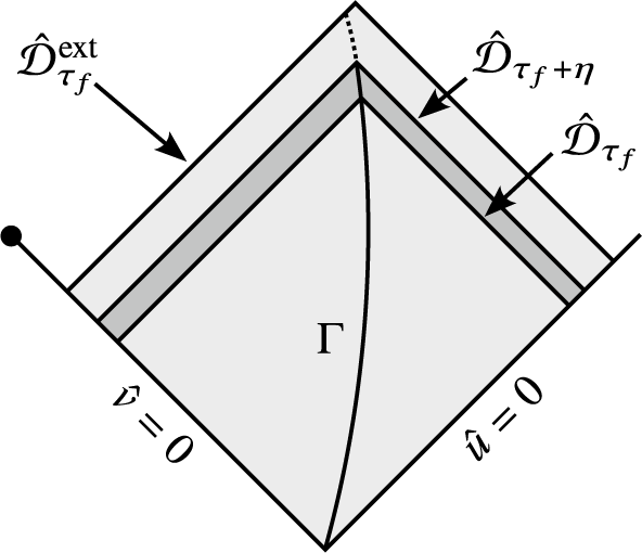


 Open access