


1. Introduction
Diffusive search for hidden targets is critically important for various physical, chemical and biological systems [Reference Dagdug, Peña and Pompa-García21, Reference Lindenberg, Oshanin and Metzler58, Reference Masoliver60, Reference Metzler, Oshanin and Redner62, Reference Redner67, Reference Schuss73]. In the most basic setting, a point-like particle (e.g., a molecule, an ion, a protein, a virus, a bacterium, etc.) undergoes diffusive motion inside a confining environment and searches for an immobile target (e.g., a catalytic site on a solid surface, a channel on a plasma membrane, a specific site on the DNA, a cell, etc.). If the target is hidden in the bulk, it is often called an interior trap or a sink, whereas a target on the boundary is referred to as a reactive patch or an escape window. In both cases, if the target is small, one usually speaks about the narrow escape problem [Reference Holcman and Schuss48, Reference Holcman and Schuss49], bearing in mind the picture of an open window, through which the particle can leave the domain and never return. Most former works were dedicated to finding and even optimising the mean first-passage time (FPT) to a single target or to a given arrangement of multiple targets [Reference Chen and Friedman12, Reference Cheviakov, Ward and Straube16, Reference Grebenkov30, Reference Grebenkov and Oshanin42, Reference Guérin, Dolgushev, Bénichou and Voituriez44, Reference Iyaniwura, Wong, Macdonald and Ward50, Reference Lindsay, Bernoff and Ward59, Reference Pillay, Ward, Peirce and Kolokolnikov65, Reference Schuss, Singer and Holcman74, Reference Singer, Schuss, Holcman and Eisenberg75]. Other relevant characteristics of the diffusive search, such as the whole distribution of the FPT [Reference Bénichou and Voituriez2, Reference Cherry, Lindsay, Navarro Hernández and Quaife13, Reference Godec and Metzler29, Reference Grebenkov, Metzler and Oshanin40, Reference Grebenkov, Metzler and Oshanin41] and Laplacian eigenvalues [Reference Cheviakov and Ward15, Reference Coombs, Straube and Ward20, Reference Kolokolnikov, Titcombe and Ward51], were also studied.
A common limitation of most former works is their emphasis either on a single target or on multiple targets of the same type. In turn, many biochemical applications involve targets of different types. For instance, signal transduction between neurones relies on diffusive search by calcium ions of a sensor protein on the vesicle with neurotransmitters inside the presynaptic bouton [Reference Guerrier and Holcman45, Reference Holcman and Schuss48, Reference Neher and Sakaba63, Reference Reva, DiGregorio and Grebenkov68, Reference Sala and Hernández-Cruz70]. While the sensor protein is the primary target, calcium ions can reversibly bind to buffer molecules inside the confining domain or leave it through calcium channels on its boundary. Both buffer molecules and channels play the role of auxiliary targets that compete for calcium ions and thus allow to control the signal transduction. More generally, the successful reaction of a diffusing particle on a “primary” target may fail due to its eventual capture by other targets or its escape.
When all targets are perfect (i.e., the reaction occurs instantly upon the first arrival), the competition between targets for a diffusing particle is characterised via diffusive fluxes, splitting probabilities and conditional FPTs [Reference Berezhkovskii, Dagdug, Lizunov, Zimmerberg and Bezrukov3, Reference Bressloff5, Reference Chevalier, Bénichou, Meyer and Voituriez14, Reference Delgado, Ward and Coombs22, Reference Felici, Filoche and Sapoval25, Reference Grebenkov32, Reference Grebenkov and Traytak43, Reference Kurella, Tzou, Coombs and Ward54, Reference Traytak76, Reference Traytak and Tachiya77]. In particular, the asymptotic behaviour of these quantities for small interior traps or absorbing patches on the boundary and the dependence on their spatial arrangement have been studied in depth. However, as the targets are not perfectly reactive in most applications [Reference Bressloff6, Reference Collins and Kimball19, Reference Erban and Chapman24, Reference Galanti, Fanelli and Piazza27, Reference Grebenkov31, Reference Grebenkov32, Reference Grebenkov35, Reference Lawley and Keener55, Reference Piazza64, Reference Sano and Tachiya71, Reference Sapoval72], their competition also depends on their reactivities. The role of partially reactive traps, as modelled by a Robin condition, is not nearly as well understood, especially in the two-dimensional case.
The problem becomes even more challenging for more intricate surface reactions, which cannot be described by the conventional Robin boundary condition on targets. We will refer to such targets as imperfect. For instance, the target reactivity can be progressively increased or decreased by encounters with a diffusing particle. Such activation or passivation processes are described within the encounter-based approach [Reference Bressloff7, Reference Bressloff8, Reference Grebenkov33, Reference Grebenkov34, Reference Grebenkov36]. In probabilistic terms, the reaction event occurs when the number of reaction attempts upon each arrival onto the target exceeds some random threshold. The probability distribution of the threshold characterises the reaction mechanism (see details in [Reference Grebenkov34]). For instance, the particular case of the exponential distribution corresponds to a partially reactive target with a constant reactivity, and its probabilistic description is equivalent to solving the diffusion equation with the Robin boundary condition. In turn, other distributions of the threshold describe more intricate surface reactions and involve integral-type boundary conditions. As shown in [Reference Grebenkov34], such PDE problems can be solved by employing spectral expansions based on the Steklov problem (see Sections 4 and 5 for its formulation and basic properties). In particular, the Steklov eigenfunctions turn out to be particularly suitable for dealing with diffusive motion in the confining domain between successive arrivals onto an imperfect target. The peculiar feature of the Steklov problem that distinguishes it from common spectral problems for the Laplacian is that the spectral parameter appears in the boundary condition. Various properties of the Steklov problem have been thoroughly investigated (see [Reference Behrndt and ter Elst1, Reference Colbois, Girouard, Gordon and Sher18, Reference Girouard and Polterovich28, Reference Hassell and Ivrii46, Reference Levitin, Mangoubi and Polterovich56] and references therein). When imperfect targets are located on the inert impenetrable boundary, one needs to combine Steklov and Neumann boundary conditions. Such a mixed Steklov-Neumann problem was already known in hydrodynamics, where it is referred to as the sloshing problem [Reference Fox and Kuttler26, Reference Henrici, Troesch and Wuytack47, Reference Kozlov and Kuznetsov53, Reference Levitin, Parnovski, Polterovich and Sher57]. In the case of a single target, the asymptotic behaviour of its eigenvalues and eigenfunctions in the small-target limit was recently studied [Reference Grebenkov38]. However, the scaling arguments and related analysis from [Reference Grebenkov38] are not directly applicable to the case of multiple targets. The asymptotic behaviour of the spectrum of the mixed Steklov-Neumann problem is thus unknown, despite the importance of its potential applications. Yet another unstudied setting concerns a single imperfect target with the Steklov condition in the presence of multiple escape windows with the Dirichlet condition. A mathematical framework for studying such an escape problem relies on the mixed Steklov-Neumann-Dirichlet problem [Reference Grebenkov37]. To our knowledge, the asymptotic behaviour of its eigenvalues and eigenfunctions in the small-target limit has not been studied previously.
In this paper, we progressively fill the gap between perfect and imperfect targets. In Section 2, we start with the conventional setting of
 $N$
absorbing sinks and study their splitting probabilities, i.e., the probability of hitting one sink before any other. This relatively simple setting allows us to introduce, in a didactic way, many notions and tools that will be employed throughout the manuscript. Even though this problem was studied in the past (see [Reference Bressloff5, Reference Chevalier, Bénichou, Meyer and Voituriez14] and references therein), we succeed in improving and generalising some earlier results. Section 3 presents an extension to partially reactive targets, in which the Dirichlet boundary condition is replaced by a Robin condition. We show how partial reactivity effectively reduces the target size. The major contributions of the paper are presented in Sections 4 and 5. In Section 4, we consider the mixed Steklov-Neumann problem for
$N$
absorbing sinks and study their splitting probabilities, i.e., the probability of hitting one sink before any other. This relatively simple setting allows us to introduce, in a didactic way, many notions and tools that will be employed throughout the manuscript. Even though this problem was studied in the past (see [Reference Bressloff5, Reference Chevalier, Bénichou, Meyer and Voituriez14] and references therein), we succeed in improving and generalising some earlier results. Section 3 presents an extension to partially reactive targets, in which the Dirichlet boundary condition is replaced by a Robin condition. We show how partial reactivity effectively reduces the target size. The major contributions of the paper are presented in Sections 4 and 5. In Section 4, we consider the mixed Steklov-Neumann problem for
 $N$
imperfect targets. For this novel problem, we obtain the asymptotic behaviour of its eigenvalues and eigenfunctions in the small-target limit. In turn, Section 5 focuses on the mixed Steklov-Neumann-Dirichlet problem, in which one target is imperfect (with Steklov condition), whereas the other targets are perfect (with Dirichlet condition). We apply matched asymptotic expansion techniques to investigate the asymptotic behaviour in the small-target limit. For all considered cases, the accuracy of the derived asymptotic formulas is illustrated on two examples: the case of two patches in an arbitrary domain and the case of
$N$
imperfect targets. For this novel problem, we obtain the asymptotic behaviour of its eigenvalues and eigenfunctions in the small-target limit. In turn, Section 5 focuses on the mixed Steklov-Neumann-Dirichlet problem, in which one target is imperfect (with Steklov condition), whereas the other targets are perfect (with Dirichlet condition). We apply matched asymptotic expansion techniques to investigate the asymptotic behaviour in the small-target limit. For all considered cases, the accuracy of the derived asymptotic formulas is illustrated on two examples: the case of two patches in an arbitrary domain and the case of
 $N$
equally spaced patches on the boundary of a disk. Our analytical results are compared with numerical solutions obtained by a finite-element method in Matlab (its home-made implementation for Steklov problems is described in [Reference Chaigneau and Grebenkov11]). In Section 6, we discuss two further extensions of the present analysis: the case of interior targets (or traps), and exterior problems for which diffusion occurs outside a compact set. In this way, we cover a wide variety of settings in which multiple small targets of different types compete for diffusing particles in planar domains. We summarise our main results in Section 7.
$N$
equally spaced patches on the boundary of a disk. Our analytical results are compared with numerical solutions obtained by a finite-element method in Matlab (its home-made implementation for Steklov problems is described in [Reference Chaigneau and Grebenkov11]). In Section 6, we discuss two further extensions of the present analysis: the case of interior targets (or traps), and exterior problems for which diffusion occurs outside a compact set. In this way, we cover a wide variety of settings in which multiple small targets of different types compete for diffusing particles in planar domains. We summarise our main results in Section 7.
2. Splitting probabilities on Dirichlet patches
To introduce the theoretical framework and tools, we begin by revisiting the classical problem of splitting probabilities, which are commonly used to characterise competition between multiple perfectly reactive targets for a diffusing particle. Although this problem has been studied previously (see [Reference Bressloff5, Reference Chevalier, Bénichou, Meyer and Voituriez14] and references therein), we will improve and generalise some earlier results.
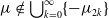
Illustration of a bounded domain
 $\Omega \subset {\mathbb{R}}^2$
with a smooth boundary
$\Omega \subset {\mathbb{R}}^2$
with a smooth boundary
 $\partial \Omega$
split into three absorbing patches
$\partial \Omega$
split into three absorbing patches
 $\Gamma _{\varepsilon _i}$
of length
$\Gamma _{\varepsilon _i}$
of length
 $2\varepsilon _i$
(in red and blue), and the remaining reflecting part
$2\varepsilon _i$
(in red and blue), and the remaining reflecting part
 $\partial \Omega _0$
(grey dashed line). For a particle starting from a point
$\partial \Omega _0$
(grey dashed line). For a particle starting from a point
 ${{\boldsymbol{x}}}\in \Omega$
, the splitting probability
${{\boldsymbol{x}}}\in \Omega$
, the splitting probability
 $S_1({{\boldsymbol{x}}})$
is the probability of hitting the blue patch
$S_1({{\boldsymbol{x}}})$
is the probability of hitting the blue patch
 $\Gamma _{\varepsilon _1}$
first.
$\Gamma _{\varepsilon _1}$
first.

Let
 $\Omega \subset {\mathbb{R}}^2$
be a bounded planar domain with a smooth boundary
$\Omega \subset {\mathbb{R}}^2$
be a bounded planar domain with a smooth boundary
 $\partial \Omega$
. Let
$\partial \Omega$
. Let
 $\{\Gamma _{\varepsilon _1}, \ldots , \Gamma _{\varepsilon _N}\}$
be
$\{\Gamma _{\varepsilon _1}, \ldots , \Gamma _{\varepsilon _N}\}$
be
 $N$
disjoint subsets of the boundary
$N$
disjoint subsets of the boundary
 $\partial \Omega$
that represent multiple patches of lengths
$\partial \Omega$
that represent multiple patches of lengths
 $2\varepsilon _1, \ldots , 2\varepsilon _N$
that are centred at boundary points
$2\varepsilon _1, \ldots , 2\varepsilon _N$
that are centred at boundary points
 ${{\boldsymbol{x}}}_1, \ldots , {{\boldsymbol{x}}}_N$
(each patch
${{\boldsymbol{x}}}_1, \ldots , {{\boldsymbol{x}}}_N$
(each patch
 $\Gamma _{\varepsilon _j}$
is connected). The remaining part of the boundary, denoted as
$\Gamma _{\varepsilon _j}$
is connected). The remaining part of the boundary, denoted as
 $\partial \Omega _0 = \partial \Omega \backslash (\Gamma _{\varepsilon _1} \cup \cdots \cup \Gamma _{\varepsilon _N})$
, is reflecting (Figure 1). We are interested in the small-target limit when all patches are small and comparable (i.e.,
$\partial \Omega _0 = \partial \Omega \backslash (\Gamma _{\varepsilon _1} \cup \cdots \cup \Gamma _{\varepsilon _N})$
, is reflecting (Figure 1). We are interested in the small-target limit when all patches are small and comparable (i.e.,
 $\varepsilon _1 \sim o(1)$
and
$\varepsilon _1 \sim o(1)$
and
 $\varepsilon _j/\varepsilon _1 \sim {\mathcal O}(1)$
). We assume that the patches are well-separated in the sense that
$\varepsilon _j/\varepsilon _1 \sim {\mathcal O}(1)$
). We assume that the patches are well-separated in the sense that
 $|{{\boldsymbol{x}}}_i - {{\boldsymbol{x}}}_j| = {\mathcal O}(1)$
for all
$|{{\boldsymbol{x}}}_i - {{\boldsymbol{x}}}_j| = {\mathcal O}(1)$
for all
 $i\ne j$
.
$i\ne j$
.
In this section, we consider that all patches
 $\Gamma _{\varepsilon _j}$
are absorbing sinks (i.e., perfectly reactive targets). For a particle started from a point
$\Gamma _{\varepsilon _j}$
are absorbing sinks (i.e., perfectly reactive targets). For a particle started from a point
 ${{\boldsymbol{x}}} \in \Omega$
, we aim at determining the splitting probability
${{\boldsymbol{x}}} \in \Omega$
, we aim at determining the splitting probability
 $S_k({{\boldsymbol{x}}})$
(
$S_k({{\boldsymbol{x}}})$
(
 $k = 1,\ldots ,N$
), i.e., the probability of the arrival onto the Dirichlet patch
$k = 1,\ldots ,N$
), i.e., the probability of the arrival onto the Dirichlet patch
 $\Gamma _{\varepsilon _k}$
before hitting any other patch. This probability satisfies the boundary value problem (BVP)
$\Gamma _{\varepsilon _k}$
before hitting any other patch. This probability satisfies the boundary value problem (BVP)
 \begin{align} \Delta S_k & = 0 \quad \textrm {in}\,\Omega , \end{align}
 \begin{align} S_k &= \delta _{j,k} \quad \textrm {on}\, \Gamma _{\varepsilon _j}, \quad j\in \lbrace {1,\ldots ,N\rbrace }, \end{align}
 \begin{align} \partial _n S_k & = 0 \quad \textrm {on}\, \partial \Omega _0, \\[6pt] \nonumber \end{align}
where
 $\Delta$
is the Laplacian,
$\Delta$
is the Laplacian,
 $\partial _n$
is the normal derivative oriented outward to the domain
$\partial _n$
is the normal derivative oriented outward to the domain
 $\Omega$
, and
$\Omega$
, and
 $\delta _{j,k}$
is the Kronecker symbol. In the analysis below,
$\delta _{j,k}$
is the Kronecker symbol. In the analysis below,
 $k\in \lbrace {1,\ldots ,N\rbrace }$
is fixed. In the small-target limit
$k\in \lbrace {1,\ldots ,N\rbrace }$
is fixed. In the small-target limit
 $\varepsilon _j\to 0$
for each
$\varepsilon _j\to 0$
for each
 $j\in \lbrace {1,\ldots ,N\rbrace }$
, we will use the method of matched asymptotic expansions for problems with logarithmic interactions [Reference Ward, Henshaw and Keller78] to approximate solutions to (2.1) that are accurate to all powers of
$j\in \lbrace {1,\ldots ,N\rbrace }$
, we will use the method of matched asymptotic expansions for problems with logarithmic interactions [Reference Ward, Henshaw and Keller78] to approximate solutions to (2.1) that are accurate to all powers of
 $1/\ln (\varepsilon _j)$
.
$1/\ln (\varepsilon _j)$
.
2.1. Inner solutions
The inner solution near each Dirichlet patch
 $\Gamma _{\varepsilon _j}$
can be found by introducing the local coordinates
$\Gamma _{\varepsilon _j}$
can be found by introducing the local coordinates
 ${\boldsymbol{y}} = \varepsilon _j^{-1} \textbf{Q}_j ({{\boldsymbol{x}}}-{{\boldsymbol{x}}}_j)$
, where
${\boldsymbol{y}} = \varepsilon _j^{-1} \textbf{Q}_j ({{\boldsymbol{x}}}-{{\boldsymbol{x}}}_j)$
, where
 $\textbf{Q}_j$
is an appropriate rotation matrix to restrict
$\textbf{Q}_j$
is an appropriate rotation matrix to restrict
 ${\boldsymbol{y}} = (y_1,y_2)$
to the upper-half-plane
${\boldsymbol{y}} = (y_1,y_2)$
to the upper-half-plane
 ${\mathbb{H}}_2 = {\mathbb{R}} \times {\mathbb{R}}_+$
(the matrix
${\mathbb{H}}_2 = {\mathbb{R}} \times {\mathbb{R}}_+$
(the matrix
 $\textbf{Q}_j$
plays no role since
$\textbf{Q}_j$
plays no role since
 $\textbf{Q}_j^\dagger \textbf{Q}_j = {\textbf{I}}$
and
$\textbf{Q}_j^\dagger \textbf{Q}_j = {\textbf{I}}$
and
 $|{\boldsymbol{y}}| = \varepsilon _j^{-1} |{{\boldsymbol{x}}}-{{\boldsymbol{x}}}_j|$
). We look for an inner solution near the patch
$|{\boldsymbol{y}}| = \varepsilon _j^{-1} |{{\boldsymbol{x}}}-{{\boldsymbol{x}}}_j|$
). We look for an inner solution near the patch
 $\Gamma _{\varepsilon _j}$
in the form
$\Gamma _{\varepsilon _j}$
in the form
 \begin{equation} S_k({{\boldsymbol{x}}}_j + \varepsilon _j \textbf{Q}_j^\dagger {\boldsymbol{y}}) = \delta _{j,k} + A_j g_\infty (\,{\boldsymbol{y}}), \quad j\in \lbrace {1,\ldots ,N\rbrace }, \end{equation}
where
 $A_j$
is an unknown constant, and
$A_j$
is an unknown constant, and
 $g_\infty (\,{\boldsymbol{y}})$
is the Green’s function satisfying the canonical BVP given by
$g_\infty (\,{\boldsymbol{y}})$
is the Green’s function satisfying the canonical BVP given by
 \begin{align} \Delta g_\infty &= 0 \quad \textrm {in}\, {\mathbb{H}}_2, \\[-8pt] \nonumber \end{align}
 \begin{align} \partial _n g_\infty &= 0 \quad \textrm {on}\, y_2 = 0, \, |y_1| \geq 1; \qquad g_\infty = 0 \quad \textrm {on}\, y_2 =0, \, |y_1| \lt 1 , \\[-8pt] \nonumber \end{align}
 \begin{align} g_\infty &\sim \ln |{\boldsymbol{y}}| + {\mathcal O}(1) \quad \textrm {as}\, |{\boldsymbol{y}}| \to \infty , \\[11pt] \nonumber \end{align}
(the subscript
 $\infty$
highlights infinite reactivity of the perfect patch, see below). The exact solution of this classical problem is given in Appendix A for completeness. The analysis below will require only the knowledge of the asymptotic behaviour of
$\infty$
highlights infinite reactivity of the perfect patch, see below). The exact solution of this classical problem is given in Appendix A for completeness. The analysis below will require only the knowledge of the asymptotic behaviour of
 $g_\infty (\,{\boldsymbol{y}})$
at infinity. We recall that the constant term in this behaviour,
$g_\infty (\,{\boldsymbol{y}})$
at infinity. We recall that the constant term in this behaviour,
 \begin{equation} g_\infty (\,{\boldsymbol{y}}) \sim \ln |{\boldsymbol{y}}| - \ln (d) + o(1) \quad \textrm {as}\, |{\boldsymbol{y}}| \to \infty , \end{equation}
is determined by the logarithmic capacity
 $d$
of the interval
$d$
of the interval
 $({-}1,1)$
, which is simply
$({-}1,1)$
, which is simply
 $d={1/2}$
. Now putting
$d={1/2}$
. Now putting
 ${\boldsymbol{y}} = \varepsilon _j^{-1} \textbf{Q}_j ({{\boldsymbol{x}}}-{{\boldsymbol{x}}}_j)$
, we get that the far-field behaviour of the inner solution is
${\boldsymbol{y}} = \varepsilon _j^{-1} \textbf{Q}_j ({{\boldsymbol{x}}}-{{\boldsymbol{x}}}_j)$
, we get that the far-field behaviour of the inner solution is
 \begin{equation} S_k \sim \delta _{j,k} + A_j \big [\ln |{{\boldsymbol{x}}}-{{\boldsymbol{x}}}_j| - \ln (\varepsilon _j d) + o(1)\big] \quad \textrm {as}\ {{\boldsymbol{x}}}\to {{\boldsymbol{x}}}_j. \end{equation}
Setting
 \begin{equation} \nu _j = - \frac {1}{\ln (\varepsilon _j d)} , \quad \mbox{with} \quad d=\frac {1}{2} , \end{equation}
we rewrite this far-field behaviour, for each
 $j \in \lbrace {1,\ldots ,N\rbrace }$
, as
$j \in \lbrace {1,\ldots ,N\rbrace }$
, as
 \begin{equation} S_k \sim \delta _{j,k} + A_j \big[\ln |{{\boldsymbol{x}}}-{{\boldsymbol{x}}}_j| + 1/\nu _j + o(1)\big] \quad \textrm {as}\,\,{{\boldsymbol{x}}}\to {{\boldsymbol{x}}}_j. \end{equation}
2.2. Outer solution and matching conditions
Now, we consider the outer problem for
 $S_k({{\boldsymbol{x}}})$
given by
$S_k({{\boldsymbol{x}}})$
given by
 \begin{align} \Delta S_k & = 0 \quad \textrm {in}\, \Omega , \\[-5pt] \nonumber \end{align}
 \begin{align} S_k & \sim \delta _{j,k} + A_j\, \bigl [\ln |{{\boldsymbol{x}}}-{{\boldsymbol{x}}}_j| + 1/\nu _j \bigr ] \quad \textrm {as}\ \ {{\boldsymbol{x}}} \to {{\boldsymbol{x}}}_j\in \partial \Omega , \quad j\in \lbrace {1,\ldots ,N\rbrace }, \\[-5pt] \nonumber \end{align}
 \begin{align} \partial _n S_k & = 0 \quad \textrm {on}\, \partial \Omega \backslash \{{{\boldsymbol{x}}}_1,\ldots ,{{\boldsymbol{x}}}_N\}. \\[11pt] \nonumber \end{align}
To find this solution, we introduce the surface Neumann Green’s function
 $G({{\boldsymbol{x}}},{\boldsymbol \xi })$
, which satisfies
$G({{\boldsymbol{x}}},{\boldsymbol \xi })$
, which satisfies
 \begin{align} \Delta G & = \frac {1}{|\Omega |} \quad \textrm {in}\, \Omega ; \quad \partial _n G = 0 \quad \textrm {on}\, \partial \Omega \backslash \{{\boldsymbol \xi }\}; \quad \int \limits _{\Omega } G({{\boldsymbol{x}}},{\boldsymbol \xi })\,d{{\boldsymbol{x}}} = 0,\\[-10pt]\nonumber \end{align}
 \begin{align} G({{\boldsymbol{x}}},{\boldsymbol \xi }) & \sim - \frac {1}{\pi } \ln |{{\boldsymbol{x}}}-{\boldsymbol \xi }| + R({\boldsymbol \xi }) + o(1) \quad \textrm {as}\, {{\boldsymbol{x}}} \to {\boldsymbol \xi }\in \partial \Omega , \end{align}
where
 $|\Omega |$
is the area of
$|\Omega |$
is the area of
 $\Omega$
, and
$\Omega$
, and
 $R({\boldsymbol \xi })$
is the regular part of
$R({\boldsymbol \xi })$
is the regular part of
 $G({{\boldsymbol{x}}},{\boldsymbol \xi })$
, defined by
$G({{\boldsymbol{x}}},{\boldsymbol \xi })$
, defined by
 \begin{equation} R({\boldsymbol \xi }) = \lim \limits _{{{\boldsymbol{x}}}\to {\boldsymbol \xi }} \biggl (G({{\boldsymbol{x}}},{\boldsymbol \xi }) + \frac {1}{\pi } \ln |{{\boldsymbol{x}}}-{\boldsymbol \xi }|\biggr ). \end{equation}
The formulation in (2.9) is equivalent to imposing that
 $\partial _n G=\delta ({{\boldsymbol{x}}}-{\boldsymbol \xi })$
on
$\partial _n G=\delta ({{\boldsymbol{x}}}-{\boldsymbol \xi })$
on
 $\partial \Omega$
where
$\partial \Omega$
where
 ${\boldsymbol \xi }\in \partial \Omega$
.
${\boldsymbol \xi }\in \partial \Omega$
.
Remark 1.
For a disk,
 $G$
and
$G$
and
 $R$
are known analytically from [Reference Kolokolnikov, Titcombe and Ward51] and [Reference Pillay, Ward, Peirce and Kolokolnikov65] (see (2.28) below). For a square domain, they can be represented in terms of rapidly converging infinite series representations (see Section 3.3 of [Reference Pillay, Ward, Peirce and Kolokolnikov65]). Similar representations can be obtained for rectangles and ellipses from the results for the interior Neumann Green’s function in Section 4.2 of [Reference Kolokolnikov, Ward and Wei52] and in Section 5 of [Reference Iyaniwura, Wong, Macdonald and Ward50], respectively, by allowing the interior source point to tend to the domain boundary (see Section F.2 for this derivation for an ellipse and Table F1). A numerical method to compute
$R$
are known analytically from [Reference Kolokolnikov, Titcombe and Ward51] and [Reference Pillay, Ward, Peirce and Kolokolnikov65] (see (2.28) below). For a square domain, they can be represented in terms of rapidly converging infinite series representations (see Section 3.3 of [Reference Pillay, Ward, Peirce and Kolokolnikov65]). Similar representations can be obtained for rectangles and ellipses from the results for the interior Neumann Green’s function in Section 4.2 of [Reference Kolokolnikov, Ward and Wei52] and in Section 5 of [Reference Iyaniwura, Wong, Macdonald and Ward50], respectively, by allowing the interior source point to tend to the domain boundary (see Section F.2 for this derivation for an ellipse and Table F1). A numerical method to compute
 $G$
and
$G$
and
 $R$
in arbitrary planar domains is described in Section 3.3 of [Reference Pillay, Ward, Peirce and Kolokolnikov65].
$R$
in arbitrary planar domains is described in Section 3.3 of [Reference Pillay, Ward, Peirce and Kolokolnikov65].
The divergence theorem applied to Eq. (2.8) yields
 \begin{equation} \sum \limits _{j=1}^N A_j = 0. \end{equation}
Under this condition, the solution to Eq. (2.8) can be written as the linear combination
 \begin{equation} S_k({{\boldsymbol{x}}}) = \chi _k - \sum \limits _{i=1}^N \pi A_i G({{\boldsymbol{x}}},{{\boldsymbol{x}}}_i) , \end{equation}
where
 $\chi _k$
is a constant to be found. Matching the inner and outer asymptotic expansions as
$\chi _k$
is a constant to be found. Matching the inner and outer asymptotic expansions as
 ${{\boldsymbol{x}}}\to {{\boldsymbol{x}}}_j$
gives
${{\boldsymbol{x}}}\to {{\boldsymbol{x}}}_j$
gives
 \begin{equation} A_j + \nu _j\left[A_j R_j + \sum \limits _{i=1 \atop i\ne j}^N G_{j,i} A_i\right] = \chi _k \nu _j - \nu _k \delta _{j,k}, \end{equation}
for
 $j\in \lbrace {1,\ldots ,N\rbrace }$
, where we have defined
$j\in \lbrace {1,\ldots ,N\rbrace }$
, where we have defined
 \begin{equation} G_{j,i} = \pi G({{\boldsymbol{x}}}_j,{{\boldsymbol{x}}}_i) \quad (i\ne j), \qquad R_j = \pi R({{\boldsymbol{x}}}_j). \end{equation}
Together with the compatibility condition (2.11), we obtain a system of
 $N+1$
linear equations that determine the unknown coefficients
$N+1$
linear equations that determine the unknown coefficients
 $A_1, \ldots ,A_N$
and
$A_1, \ldots ,A_N$
and
 $\chi _k$
.
$\chi _k$
.
2.3. Matrix reformulation and general solution
To proceed, we introduce the following vectors and matrices of sizes
 $N\times 1$
and
$N\times 1$
and
 $N\times N$
:
$N\times N$
:
 \begin{align} {\textbf{e}} = \left (\begin{array}{c} 1 \\ 1 \\ \cdots \\ 1 \\ \end{array}\right ), \quad {\boldsymbol \nu } = \left (\begin{array}{c@{\quad}c@{\quad}c@{\quad}c} \nu _1 & 0 & \cdots & 0 \\ 0 & \nu _2 & \cdots & 0 \\ \cdots &\cdots &\cdots &\cdots \\ 0 & 0 &\cdots & \nu _N \\ \end{array}\right ), \quad {\textbf{G}} = \left (\begin{array}{c@{\quad}c@{\quad}c@{\quad}c} R_1 & G_{1,2} & \cdots & G_{1,N} \\ G_{2,1} & R_2 & \cdots & G_{2,N} \\ \cdots &\cdots &\cdots &\cdots \\ G_{N,1} & G_{N,2} &\cdots & R_N \\ \end{array}\right )\, \quad {\textbf{e}}_k = \left (\begin{array}{c} 0 \\ 1 \\ \cdots \\ 0 \\ \end{array}\right ),\nonumber\\[4pt] \end{align}
where
 $1$
stands on the
$1$
stands on the
 $k$
-th row of the vector
$k$
-th row of the vector
 ${\textbf{e}}_k$
.
${\textbf{e}}_k$
.
In terms of this notation, the system (2.13) is written in matrix form as
 \begin{equation} {\textbf{A}} + {\boldsymbol \nu } {\textbf{G}} {\textbf{A}} = \chi _k {\boldsymbol \nu } {\textbf{e}} - {\boldsymbol \nu } {\textbf{e}}_k . \end{equation}
Applying
 ${\textbf{e}}^\dagger$
on the left, we isolate
${\textbf{e}}^\dagger$
on the left, we isolate
 $\chi _k$
as
$\chi _k$
as
 \begin{equation} \chi _k = \frac {{\textbf{e}}^\dagger {\boldsymbol \nu } {\textbf{G}} {\textbf{A}}}{\bar {\nu }} + \frac {\nu _k}{\bar {\nu }} , \end{equation}
where we used
 ${\textbf{e}}^\dagger {\textbf{A}} = 0$
due to Eq. (2.11), and defined
${\textbf{e}}^\dagger {\textbf{A}} = 0$
due to Eq. (2.11), and defined
 \begin{equation} \bar {\nu } = {\textbf{e}}^\dagger {\boldsymbol \nu } {\textbf{e}} = \sum \limits _{j=1}^N \nu _j . \end{equation}
Eliminating
 $\chi _k$
from Eq. (2.16), we get a matrix equation for
$\chi _k$
from Eq. (2.16), we get a matrix equation for
 $\textbf{A}$
given by
$\textbf{A}$
given by
 \begin{equation} ({\textbf{I}} + {\boldsymbol \nu } {\textbf{G}}) {\textbf{A}} - {\boldsymbol \nu } {\textbf{e}} \, \frac {{\textbf{e}}^\dagger {\boldsymbol \nu } {\textbf{G}} {\textbf{A}}}{\bar {\nu }} = \frac {\nu _k}{\bar {\nu }} {\boldsymbol \nu } {\textbf{e}} - \nu _k {\textbf{e}}_k . \end{equation}
By introducing the matrices
 ${\textbf{M}}_0$
and
${\textbf{M}}_0$
and
 $\textbf{E}$
by
$\textbf{E}$
by
 \begin{equation} {\textbf{M}}_0 = {\textbf{I}} + \biggl ({\textbf{I}} - \frac {{\boldsymbol \nu } {\textbf{E}}}{\bar {\nu }}\biggr ) {\boldsymbol \nu } {\textbf{G}}, \qquad {\textbf{E}} = {\textbf{e}} {\textbf{e}}^\dagger , \end{equation}
the solution to Eq. (2.19) is
 \begin{equation} {\textbf{A}} = \frac {\nu _k}{\bar {\nu }} {\textbf{M}}_0^{-1} \bigl ({\boldsymbol \nu } {\textbf{e}} - \bar {\nu } {\textbf{e}}_k \bigr ), \end{equation}
where
 ${\textbf{M}}_0^{-1}$
is the inverse of
${\textbf{M}}_0^{-1}$
is the inverse of
 ${\textbf{M}}_0$
. In fact, in the small-target limit, all
${\textbf{M}}_0$
. In fact, in the small-target limit, all
 $\nu _j \ll 1$
so that
$\nu _j \ll 1$
so that
 ${\textbf{M}}_0$
is a small perturbation of the identity matrix
${\textbf{M}}_0$
is a small perturbation of the identity matrix
 $\textbf{I}$
and is thus invertible. Once the coefficients
$\textbf{I}$
and is thus invertible. Once the coefficients
 $A_i$
are found, the constant
$A_i$
are found, the constant
 $\chi _k$
follows from Eq. (2.17). As a consequence, the splitting probability
$\chi _k$
follows from Eq. (2.17). As a consequence, the splitting probability
 $S_k({{\boldsymbol{x}}})$
is fully determined via the representation (2.12). This is the main result of this section. The shape of the confining domain
$S_k({{\boldsymbol{x}}})$
is fully determined via the representation (2.12). This is the main result of this section. The shape of the confining domain
 $\Omega$
and the arrangement of Dirichlet patches are captured by the matrix
$\Omega$
and the arrangement of Dirichlet patches are captured by the matrix
 $\textbf{G}$
, whereas the sizes of patches are accounted for via the matrix
$\textbf{G}$
, whereas the sizes of patches are accounted for via the matrix
 $\boldsymbol \nu$
. When the surface Neumann Green’s function is known analytically, a numerical computation of the coefficients
$\boldsymbol \nu$
. When the surface Neumann Green’s function is known analytically, a numerical computation of the coefficients
 $A_i$
and
$A_i$
and
 $\chi _k$
is fast, at least if the number of targets is not too large. We emphasise that the solution
$\chi _k$
is fast, at least if the number of targets is not too large. We emphasise that the solution
 $\textbf{A}$
in (2.21) to the linear system (2.19) has accounted for all logarithmic correction terms in the asymptotic expansion of the splitting probability. This technique for effectively summing what otherwise would be an infinite logarithmic expansion in powers of
$\textbf{A}$
in (2.21) to the linear system (2.19) has accounted for all logarithmic correction terms in the asymptotic expansion of the splitting probability. This technique for effectively summing what otherwise would be an infinite logarithmic expansion in powers of
 $\nu _k$
was developed in [Reference Ward, Henshaw and Keller78], and has been used in other contexts (see [Reference Coombs, Straube and Ward20, Reference Kurella, Tzou, Coombs and Ward54, Reference Pillay, Ward, Peirce and Kolokolnikov65]).
$\nu _k$
was developed in [Reference Ward, Henshaw and Keller78], and has been used in other contexts (see [Reference Coombs, Straube and Ward20, Reference Kurella, Tzou, Coombs and Ward54, Reference Pillay, Ward, Peirce and Kolokolnikov65]).
We further emphasise that Eq. (2.12) is only applicable in the outer region, i.e., when
 $|{{\boldsymbol{x}}}-{{\boldsymbol{x}}}_j| \gg {\mathcal O}(\varepsilon _j)$
for all
$|{{\boldsymbol{x}}}-{{\boldsymbol{x}}}_j| \gg {\mathcal O}(\varepsilon _j)$
for all
 $j \in \lbrace {1,\ldots ,N\rbrace }$
. In turn, if the starting point
$j \in \lbrace {1,\ldots ,N\rbrace }$
. In turn, if the starting point
 ${\boldsymbol{x}}$
is too close to
${\boldsymbol{x}}$
is too close to
 ${{\boldsymbol{x}}}_j$
, this asymptotic formula may give wrong values (e.g., negative or exceeding
${{\boldsymbol{x}}}_j$
, this asymptotic formula may give wrong values (e.g., negative or exceeding
 $1$
). In practice, the outer solution can be capped by
$1$
). In practice, the outer solution can be capped by
 $0$
and
$0$
and
 $1$
to avoid such invalid values, i.e., one can use
$1$
to avoid such invalid values, i.e., one can use
 $\max \{0, \min \{1, S_k({{\boldsymbol{x}}})\}\}$
instead of
$\max \{0, \min \{1, S_k({{\boldsymbol{x}}})\}\}$
instead of
 $S_k({{\boldsymbol{x}}})$
. We remark that if an accurate approximation of the splitting probability is needed near the patch, one has to use the corresponding inner solution.
$S_k({{\boldsymbol{x}}})$
. We remark that if an accurate approximation of the splitting probability is needed near the patch, one has to use the corresponding inner solution.
We also note that the constant
 $\chi _k$
can be interpreted as the volume-averaged splitting probability. In fact, if the starting point
$\chi _k$
can be interpreted as the volume-averaged splitting probability. In fact, if the starting point
 ${\boldsymbol{x}}$
is not fixed but uniformly distributed in
${\boldsymbol{x}}$
is not fixed but uniformly distributed in
 $\Omega$
, the average over the starting point yields
$\Omega$
, the average over the starting point yields
 \begin{equation} \overline {S}_k = \frac {1}{|\Omega |} \int \limits _{\Omega } S_k({{\boldsymbol{x}}}) \, d{{\boldsymbol{x}}} = \chi _k , \end{equation}
where we used
 $\int _{\Omega } G({{\boldsymbol{x}}},{{\boldsymbol{x}}}_i)\, d{{\boldsymbol{x}}}=0$
.
$\int _{\Omega } G({{\boldsymbol{x}}},{{\boldsymbol{x}}}_i)\, d{{\boldsymbol{x}}}=0$
.
2.4. Example of two patches
In the case of two targets (
 $N = 2$
), the matrix
$N = 2$
), the matrix
 ${\textbf{M}}_0$
from Eq. (2.20) reads
${\textbf{M}}_0$
from Eq. (2.20) reads
 \begin{equation} {\textbf{M}}_0 = {\textbf{I}} + \gamma \left (\begin{array}{c@{\quad}c} R_1 - G_{1,2} & G_{1,2} - R_2 \\[4pt] G_{1,2} - R_1 & R_2 - G_{1,2} \\ \end{array}\right ), \end{equation}
where
 $\gamma = \nu _1 \nu _2/(\nu _1 + \nu _2)$
. The inverse of this matrix is
$\gamma = \nu _1 \nu _2/(\nu _1 + \nu _2)$
. The inverse of this matrix is
 \begin{equation} {\textbf{M}}_0^{-1} = \frac {1}{1 + \gamma (R_1 + R_2 - 2G_{1,2})} \left ( {\textbf{I}} + \gamma \left (\begin{array}{c@{\quad}c} R_2 - G_{1,2} & R_2 -G_{1,2} \\[4pt] R_1 -G_{1,2} & R_1 - G_{1,2} \\ \end{array}\right ) \right ) . \end{equation}
Substituting this expression into Eq. (2.21), we find for
 $k = 1$
that
$k = 1$
that
 \begin{equation} -A_1 = A_2 = \biggl (\frac {1}{\nu _1} + \frac {1}{\nu _2} + \bigl [R_1 + R_2 - 2G_{1,2}\bigr ]\biggr )^{-1} . \end{equation}
Then, by using Eq. (2.17) we determine
 $\chi _1$
as
$\chi _1$
as
 \begin{equation} \chi _1 = \frac {\nu _1 - A_2 \nu _1 (R_1 - G_{1,2}) + A_2\nu _2 (R_2 - G_{1,2})}{\nu _1+\nu _2} , \end{equation}
which can be further simplified as
 \begin{equation} \chi _1 = \frac {1/\nu _2 + (R_2 - G_{1,2})}{1/\nu _1 + 1/\nu _2 + (R_1 + R_2 - 2G_{1,2})} . \end{equation}
For instance, if
 $\Omega$
is the unit disk, the surface Neumann Green’s function is well known [Reference Pillay, Ward, Peirce and Kolokolnikov65]:
$\Omega$
is the unit disk, the surface Neumann Green’s function is well known [Reference Pillay, Ward, Peirce and Kolokolnikov65]:
 \begin{equation} G({{\boldsymbol{x}}},{\boldsymbol \xi }) = - \frac {1}{\pi } \ln |{{\boldsymbol{x}}}-{\boldsymbol \xi }| + \frac {|{{\boldsymbol{x}}}|^2}{4\pi } - \frac {1}{8\pi } , \quad R({\boldsymbol \xi }) = \frac {1}{8\pi } . \end{equation}
Substitution of these expressions into Eqs. (2.25, 2.27) yields
 \begin{align} -A_1 = A_2 & = \left({-}\ln (\varepsilon _1\varepsilon _2) + 2\ln (2) + 2\ln |{{\boldsymbol{x}}}_1-{{\boldsymbol{x}}}_2|\right)^{-1}, \\[-8pt] \nonumber \end{align}
 \begin{align} \chi _1 & = \frac {-\ln (\varepsilon _2/2) + \ln |{{\boldsymbol{x}}}_1-{{\boldsymbol{x}}}_2|} {-\ln (\varepsilon _1\varepsilon _2/4) + 2\ln |{{\boldsymbol{x}}}_1-{{\boldsymbol{x}}}_2|} , \\[8pt] \nonumber \end{align}
and we conclude that
 \begin{equation} S_1({{\boldsymbol{x}}}) = \chi _1 + A_2 \ln \biggl (\frac {|{{\boldsymbol{x}}}-{{\boldsymbol{x}}}_2|}{|{{\boldsymbol{x}}}-{{\boldsymbol{x}}}_1|} \biggr ). \end{equation}
We can easily check that
 $S_1({{\boldsymbol{x}}})$
approaches
$S_1({{\boldsymbol{x}}})$
approaches
 $0$
[resp.,
$0$
[resp.,
 $1$
] as
$1$
] as
 $\varepsilon _1\to 0$
[resp.,
$\varepsilon _1\to 0$
[resp.,
 $\varepsilon _2 \to 0$
], as expected.
$\varepsilon _2 \to 0$
], as expected.
In the special case of two identical targets,
 $\nu _1 = \nu _2 = \nu$
, one has
$\nu _1 = \nu _2 = \nu$
, one has
 $\chi _1 = 1/2$
and
$\chi _1 = 1/2$
and
 $A_2 = 1/(2/\nu + 2\ln |{{\boldsymbol{x}}}_1-{{\boldsymbol{x}}}_2|)$
so that
$A_2 = 1/(2/\nu + 2\ln |{{\boldsymbol{x}}}_1-{{\boldsymbol{x}}}_2|)$
so that
 \begin{equation} S_1({{\boldsymbol{x}}}) = \frac 12 \biggl [1 + \frac {\nu }{1 + \nu \ln |{{\boldsymbol{x}}}_1-{{\boldsymbol{x}}}_2|} \ln \biggl (\frac {|{{\boldsymbol{x}}}-{{\boldsymbol{x}}}_2|}{|{{\boldsymbol{x}}}-{{\boldsymbol{x}}}_1|}\biggr )\biggr ]. \end{equation}
We remark that if we were to expand the denominator of the second term into a Taylor series in powers of
 $\nu \ll 1$
up to
$\nu \ll 1$
up to
 ${\mathcal O}(\nu ^2)$
, we would recover the truncated approximation given in Eq. (98) from [Reference Chevalier, Bénichou, Meyer and Voituriez14]. However, as
${\mathcal O}(\nu ^2)$
, we would recover the truncated approximation given in Eq. (98) from [Reference Chevalier, Bénichou, Meyer and Voituriez14]. However, as
 $\nu = -1/\ln (\varepsilon /2)$
is not necessarily small enough, our new result Eq. (2.31) that incorporates all logarithmic terms is preferable to using the previous truncated approximation from [Reference Chevalier, Bénichou, Meyer and Voituriez14].
$\nu = -1/\ln (\varepsilon /2)$
is not necessarily small enough, our new result Eq. (2.31) that incorporates all logarithmic terms is preferable to using the previous truncated approximation from [Reference Chevalier, Bénichou, Meyer and Voituriez14].
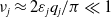
Figure 2 illustrates the splitting probability
 $S_1({{\boldsymbol{x}}})$
from Eq. (2.30). As explained earlier, we plot the capped version of this quantity,
$S_1({{\boldsymbol{x}}})$
from Eq. (2.30). As explained earlier, we plot the capped version of this quantity,
 $\max \{0, \min \{1, S_1({{\boldsymbol{x}}})\}\}$
, to avoid invalid values near two patches. Expectedly,
$\max \{0, \min \{1, S_1({{\boldsymbol{x}}})\}\}$
, to avoid invalid values near two patches. Expectedly,
 $S_1({{\boldsymbol{x}}})$
increases as
$S_1({{\boldsymbol{x}}})$
increases as
 ${\boldsymbol{x}}$
gets closer to the first patch (red arc) and decreases as
${\boldsymbol{x}}$
gets closer to the first patch (red arc) and decreases as
 ${\boldsymbol{x}}$
gets closer to the second patch (blue arc). However, as the outer solution (2.30) is not applicable in the vicinity of these patches, we can observe some discrepancy, e.g.,
${\boldsymbol{x}}$
gets closer to the second patch (blue arc). However, as the outer solution (2.30) is not applicable in the vicinity of these patches, we can observe some discrepancy, e.g.,
 $S_1({{\boldsymbol{x}}})$
does not vanish on the second patch, as it should. To amend this discrepancy, we can use the inner solution when
$S_1({{\boldsymbol{x}}})$
does not vanish on the second patch, as it should. To amend this discrepancy, we can use the inner solution when
 $|{{\boldsymbol{x}}}-{{\boldsymbol{x}}}_j| \lesssim \varepsilon _j$
.
$|{{\boldsymbol{x}}}-{{\boldsymbol{x}}}_j| \lesssim \varepsilon _j$
.
Splitting probability
 $S_1({{\boldsymbol{x}}})$
, given by Eq. (2.30), for the unit disk with two Dirichlet patches of length
$S_1({{\boldsymbol{x}}})$
, given by Eq. (2.30), for the unit disk with two Dirichlet patches of length
 $2\varepsilon _1 = 0.2$
(red) and
$2\varepsilon _1 = 0.2$
(red) and
 $2\varepsilon _2 = 0.4$
(blue). Note that
$2\varepsilon _2 = 0.4$
(blue). Note that
 $S_1({{\boldsymbol{x}}})$
was capped by
$S_1({{\boldsymbol{x}}})$
was capped by
 $0$
and
$0$
and
 $1$
, i.e., we plotted
$1$
, i.e., we plotted
 $\max \{0, \min \{1, S_1({{\boldsymbol{x}}})\}\}$
.
$\max \{0, \min \{1, S_1({{\boldsymbol{x}}})\}\}$
.

2.5. Example of equally spaced identical patches on the boundary of the unit disk
If there are
 $N$
identical targets, one has
$N$
identical targets, one has
 $\nu _j = \nu$
so that
$\nu _j = \nu$
so that
 ${\boldsymbol \nu } = \nu {\textbf{I}}$
,
${\boldsymbol \nu } = \nu {\textbf{I}}$
,
 $\bar {\nu } = N \nu$
, and thus
$\bar {\nu } = N \nu$
, and thus
 ${\textbf{M}}_0 = {\textbf{I}} + \nu ({\textbf{I}} - {\textbf{E}}/N) {\textbf{G}}$
from Eq. (2.20). Moreover, if the patches are equally spaced on the boundary of the unit circle, the matrix
${\textbf{M}}_0 = {\textbf{I}} + \nu ({\textbf{I}} - {\textbf{E}}/N) {\textbf{G}}$
from Eq. (2.20). Moreover, if the patches are equally spaced on the boundary of the unit circle, the matrix
 $\textbf{G}$
defined in Eq. (2.15) is circulant and symmetric. As a consequence, its eigenvectors can be written as
$\textbf{G}$
defined in Eq. (2.15) is circulant and symmetric. As a consequence, its eigenvectors can be written as
 \begin{equation} \textbf{q}_j = \frac {1}{\sqrt {N}} \bigl (\omega ^{-j}, \omega ^{-2j}, \ldots , \omega ^{-Nj}\bigr )^\dagger , \qquad j\in \lbrace {1,\ldots ,N\rbrace }, \end{equation}
where
 $\omega = e^{2\pi i/N}$
, and the transposition
$\omega = e^{2\pi i/N}$
, and the transposition
 $\dagger$
now denotes the Hermitian conjugate. Upon taking the real and imaginary parts of
$\dagger$
now denotes the Hermitian conjugate. Upon taking the real and imaginary parts of
 $\textbf{q}_j$
, the resulting real-valued eigenvectors form an orthonormal basis in
$\textbf{q}_j$
, the resulting real-valued eigenvectors form an orthonormal basis in
 ${\mathbb{R}}^{N}$
since
${\mathbb{R}}^{N}$
since
 $\textbf{G}$
is symmetric. Let us denote by
$\textbf{G}$
is symmetric. Let us denote by
 $\kappa _j$
the associated eigenvalues of
$\kappa _j$
the associated eigenvalues of
 $\textbf{G}$
:
$\textbf{G}$
:
 \begin{equation} \kappa _j = R_1 + \sum \limits _{m=1}^{N-1} \omega ^{mj} \, G_{1,1+m}, \qquad j\in \lbrace {1,\ldots ,N\rbrace }. \end{equation}
For any
 $j \in \lbrace {1,\ldots ,N-1\rbrace }$
, we get
$j \in \lbrace {1,\ldots ,N-1\rbrace }$
, we get
 \begin{equation} {\textbf{M}}_0 \textbf{q}_j = \bigl ({\textbf{I}} + \nu [{\textbf{I}} - {\textbf{E}}/N]\bigr ) \kappa _j \textbf{q}_j = (1 + \nu \kappa _j) \textbf{q}_j , \end{equation}
because
 ${\textbf{E}} \textbf{q}_j = {\textbf{e}} {\textbf{e}}^\dagger \textbf{q}_j = 0$
for any
${\textbf{E}} \textbf{q}_j = {\textbf{e}} {\textbf{e}}^\dagger \textbf{q}_j = 0$
for any
 $1 \leq j \leq N-1$
due to orthogonality of
$1 \leq j \leq N-1$
due to orthogonality of
 $\textbf{q}_j$
to
$\textbf{q}_j$
to
 $\textbf{q}_N = {\textbf{e}}/\sqrt {N}$
. As a consequence, each
$\textbf{q}_N = {\textbf{e}}/\sqrt {N}$
. As a consequence, each
 $\textbf{q}_j$
with
$\textbf{q}_j$
with
 $j\in \lbrace {1,\ldots ,N-1\rbrace }$
is also the eigenvector of
$j\in \lbrace {1,\ldots ,N-1\rbrace }$
is also the eigenvector of
 ${\textbf{M}}_0$
, associated to the eigenvalue
${\textbf{M}}_0$
, associated to the eigenvalue
 $1 + \nu \kappa _j$
. In addition, we have
$1 + \nu \kappa _j$
. In addition, we have
 \begin{equation} {\textbf{M}}_0 \textbf{q}_N = \bigl ({\textbf{I}} + \nu [{\textbf{I}} - {\textbf{E}}/N]\bigr ) \kappa _N \textbf{q}_N = \textbf{q}_N , \end{equation}
since
 ${\textbf{E}} \textbf{q}_N /N = \textbf{q}_N$
. Therefore,
${\textbf{E}} \textbf{q}_N /N = \textbf{q}_N$
. Therefore,
 $\textbf{q}_N$
is the eigenvector of
$\textbf{q}_N$
is the eigenvector of
 ${\textbf{M}}_0$
associated with the eigenvalue
${\textbf{M}}_0$
associated with the eigenvalue
 $1$
. We use this spectral information to invert the matrix
$1$
. We use this spectral information to invert the matrix
 ${\textbf{M}}_0$
as
${\textbf{M}}_0$
as
 \begin{equation} {\textbf{M}}_0^{-1} = \textbf{q}_N \textbf{q}_N^\dagger + \sum \limits _{j=1}^{N-1} \textbf{q}_j (1 + \nu \kappa _j)^{-1} \textbf{q}_j^\dagger . \end{equation}
Substituting this spectral representation into Eq. (2.21), we get
 \begin{equation} {\textbf{A}} = - \nu \sum \limits _{j=1}^{N-1} \textbf{q}_j (1 + \nu \kappa _j)^{-1} \textbf{q}_j^\dagger {\textbf{e}}_k, \end{equation}
where we used the orthogonality of the eigenvectors
 $\textbf{q}_j$
. Substitution of this expression into Eq. (2.17) yields
$\textbf{q}_j$
. Substitution of this expression into Eq. (2.17) yields
 $\chi _k = 1/N$
. This is consistent with the interpretation of
$\chi _k = 1/N$
. This is consistent with the interpretation of
 $\chi _k$
as the volume-averaged splitting probability: when all patches are identical and equally spaced on the boundary of the unit disk, they are equivalent from the uniformly distributed starting point, so that
$\chi _k$
as the volume-averaged splitting probability: when all patches are identical and equally spaced on the boundary of the unit disk, they are equivalent from the uniformly distributed starting point, so that
 $\overline {S}_k = 1/N$
from Eq. (2.22).
$\overline {S}_k = 1/N$
from Eq. (2.22).
To complete this example, we will simplify Eq. (2.33) by using the explicit form (2.28) of the surface Neumann Green’s function for the unit disk. Since the centres of the patches
 ${{\boldsymbol{x}}}_j$
are equally spaced on the domain boundary, we have
${{\boldsymbol{x}}}_j$
are equally spaced on the domain boundary, we have
 ${{\boldsymbol{x}}}_j = e^{2\pi i(\,j-1)/N} = \omega ^{\,j-1}$
for
${{\boldsymbol{x}}}_j = e^{2\pi i(\,j-1)/N} = \omega ^{\,j-1}$
for
 $j\in \lbrace {1,\ldots ,N\rbrace }$
. In this way, substituting Eq. (2.28) into Eq. (2.33), we get
$j\in \lbrace {1,\ldots ,N\rbrace }$
. In this way, substituting Eq. (2.28) into Eq. (2.33), we get
 \begin{equation} \kappa _j = \frac {1}{8}\sum _{m=0}^{N-1}\omega ^{\,jm} - \sum \limits _{m=1}^{N-1} \omega ^{mj} \ln \vert 1 - \omega ^m\vert , \qquad j\in \lbrace {1,\ldots ,N\rbrace } , \end{equation}
where we interpret points as complex numbers and
 $|z|$
as the modulus of
$|z|$
as the modulus of
 $z$
. For
$z$
. For
 $j=N$
, for which
$j=N$
, for which
 $\omega ^{Nm}=1$
, we get
$\omega ^{Nm}=1$
, we get
 \begin{equation} \kappa _N = \frac {N}{8} - \ln \left \vert \prod _{m=1}^{N-1}(1-\omega ^m)\right \vert = \frac {N}{8}-\ln {N} , \end{equation}
where the product in Eq. (2.39) was evaluated by using the roots of unity together with L’Hopital’s rule to get
 $\lim _{z\to 1} {(z^N-1)/(z-1)}=N=\prod _{m=1}^{N-1}(1-\omega ^m)$
. For
$\lim _{z\to 1} {(z^N-1)/(z-1)}=N=\prod _{m=1}^{N-1}(1-\omega ^m)$
. For
 $j\lt N$
, the first term in Eq. (2.38) vanishes and we obtain
$j\lt N$
, the first term in Eq. (2.38) vanishes and we obtain
 \begin{equation} \kappa _j = - \sum \limits _{m=1}^{N-1} \omega ^{mj} \ln |1 - \omega ^m|, \qquad j\in \lbrace {1,\ldots ,N-1\rbrace } , \end{equation}
which reduces after some simplifications to
 \begin{equation} \kappa _j = \ln {2} - \sum _{m=1}^{N-1}\cos \left (\frac {2\pi j m}{N}\right ) \ln \left [ \sin \left (\frac {\pi m}{N}\right ) \right ], \end{equation}
for
 $j\in \lbrace {1,\ldots ,N-1\rbrace }$
. The asymptotic behaviour of
$j\in \lbrace {1,\ldots ,N-1\rbrace }$
. The asymptotic behaviour of
 $\kappa _j$
for large
$\kappa _j$
for large
 $N$
is derived in Appendix B.
$N$
is derived in Appendix B.
3. Splitting probability on Robin patches
In most applications, targets are not perfectly reactive [Reference Bressloff6, Reference Collins and Kimball19, Reference Erban and Chapman24, Reference Galanti, Fanelli and Piazza27, Reference Grebenkov31, Reference Grebenkov32, Reference Grebenkov35, Reference Lawley and Keener55, Reference Piazza64, Reference Sano and Tachiya71, Reference Sapoval72]. Starting from Collins and Kimball [Reference Collins and Kimball19], partial reactivity is usually implemented by replacing a Dirichlet boundary condition by a Robin condition. In the case of splitting probabilities, a straightforward generalisation of the previous setting consists in replacing Dirichlet boundary condition (2.1b) by the Robin boundary condition:
 \begin{equation} \partial _n S_k + q_j S_k = q_j \delta _{j,k} \quad \textrm {on}\, \Gamma _{\varepsilon _j}, \qquad j\in \lbrace {1,\ldots ,N\rbrace }, \end{equation}
where the constant
 $0 \lt q_j \lt \infty$
characterises the reactivity of the
$0 \lt q_j \lt \infty$
characterises the reactivity of the
 $j$
-th patch
$j$
-th patch
 $\Gamma _{\varepsilon _j}$
. Here, we excluded the limit
$\Gamma _{\varepsilon _j}$
. Here, we excluded the limit
 $q_j = 0$
that would correspond to an inert patch that could be treated as a part of the reflecting boundary
$q_j = 0$
that would correspond to an inert patch that could be treated as a part of the reflecting boundary
 $\partial \Omega _0$
. The Dirichlet condition is recovered in the limit
$\partial \Omega _0$
. The Dirichlet condition is recovered in the limit
 $q_j \to +\infty$
.
$q_j \to +\infty$
.
The change of the boundary condition on the patch is a local effect that does not impact the outer solution. In turn, the inner solution near each patch
 $\Gamma _{\varepsilon _j}$
in Eq. (2.2) should now be replaced by
$\Gamma _{\varepsilon _j}$
in Eq. (2.2) should now be replaced by
 \begin{equation} S_k({{\boldsymbol{x}}}_j + \varepsilon _j \textbf{Q}_j^\dagger {\boldsymbol{y}}) = \delta _{j,k} + A_j g_{\varepsilon _j q_j}(\,{\boldsymbol{y}}), \qquad j\in \lbrace {1,\ldots ,N\rbrace }, \end{equation}
where
 $g_{\mu }(\,{\boldsymbol{y}})$
is the Robin Green’s function, which satisfies
$g_{\mu }(\,{\boldsymbol{y}})$
is the Robin Green’s function, which satisfies
 \begin{align} \Delta g_{\mu } & = 0 \quad \textrm {in}\, {\mathbb{H}}_2, \\[-10pt] \nonumber \end{align}
 \begin{align} \partial _n g_{\mu } & = 0 \quad \textrm {on}\, y_2 = 0, \, |y_1| \geq 1;\qquad \partial _n g_{\mu } + \mu g_{\mu } = 0 \quad \textrm {on}\, y_2 =0, \, |y_1| \lt 1, \\[-10pt] \nonumber \end{align}
 \begin{align} g_{\mu } & \sim \ln |{\boldsymbol{y}}| + {\mathcal O}(1) \quad \textrm {as}\, |{\boldsymbol{y}}| \to \infty . \\[8pt] \nonumber \end{align}
In Appendix C, we derive a spectral expansion for this Green’s function:
 \begin{equation} g_{\mu }(\,{\boldsymbol{y}}) = g_\infty (\,{\boldsymbol{y}}) + \pi \sum \limits _{k=0}^\infty \frac {\Psi _{2k}(\infty )}{\mu _{2k} + \mu } \Psi _{2k}(\,{\boldsymbol{y}}), \end{equation}
for any
 $\mu \notin \bigcup _{k=0}^\infty \{- \mu _{2k}\}$
. Here,
$\mu \notin \bigcup _{k=0}^\infty \{- \mu _{2k}\}$
. Here,
 $\mu _k$
and
$\mu _k$
and
 $\Psi _k(\,{\boldsymbol{y}})$
are the eigenvalues and eigenfunctions of the auxiliary Steklov-Neumann problem in the upper-half-plane:
$\Psi _k(\,{\boldsymbol{y}})$
are the eigenvalues and eigenfunctions of the auxiliary Steklov-Neumann problem in the upper-half-plane:
 \begin{align} \Delta \Psi _k & = 0 \quad \textrm {in}\, {\mathbb{H}}_2 , \\[-10pt] \nonumber \end{align}
 \begin{align} \partial _n \Psi _k & = \mu _k \Psi _k \quad \textrm {on}\, y_2 = 0, \, |y_1| \lt 1; \qquad \partial _n \Psi _k = 0 \quad \textrm {on}\, y_2 = 0, \, |y_1| \geq 1, \\[-10pt] \nonumber \end{align}
 \begin{align} \Psi _k & = {\mathcal O}(1) \quad \textrm {as}\, |{\boldsymbol{y}}|\to \infty . \\[8pt] \nonumber \end{align}
An efficient numerical procedure for computing these eigenmodes is summarised in Appendix D. Once tabulated, these eigenfunctions play a role of ‘special functions’, like orthogonal polynomials.
(a) Function
 ${\mathcal{C}}(\mu )$
from Eq. (3.7), in which the infinite series is truncated either to 50 terms (solid line) or to 10 terms (crosses), to highlight the accuracy of both truncations. Filled circles indicate the values
${\mathcal{C}}(\mu )$
from Eq. (3.7), in which the infinite series is truncated either to 50 terms (solid line) or to 10 terms (crosses), to highlight the accuracy of both truncations. Filled circles indicate the values
 $-\mu _{2k}$
, at which
$-\mu _{2k}$
, at which
 ${\mathcal{C}}(\mu )$
diverges. Dash-dotted line outlines the asymptotic limit
${\mathcal{C}}(\mu )$
diverges. Dash-dotted line outlines the asymptotic limit
 $\ln (2)$
of
$\ln (2)$
of
 ${\mathcal{C}}(\mu )$
as
${\mathcal{C}}(\mu )$
as
 $\mu \to \infty$
. (b) Comparison of
$\mu \to \infty$
. (b) Comparison of
 ${\mathcal{C}}(\mu )$
and its approximation (3.10), which is accurate over a broad range of
${\mathcal{C}}(\mu )$
and its approximation (3.10), which is accurate over a broad range of
 $\mu$
.
$\mu$
.

As a consequence, Eq. (3.4) determines the constant term
 ${\mathcal{C}}(\mu )$
in the asymptotic behaviour of
${\mathcal{C}}(\mu )$
in the asymptotic behaviour of
 $g_\mu (\,{\boldsymbol{y}})$
at infinity, defined by
$g_\mu (\,{\boldsymbol{y}})$
at infinity, defined by
 \begin{equation} g_\mu (\,{\boldsymbol{y}}) \sim \ln |{\boldsymbol{y}}| + {\mathcal{C}}(\mu ) + o(1) \quad \textrm {as}\, |{\boldsymbol{y}}| \to \infty . \end{equation}
In the limit
 $|{\boldsymbol{y}}| \to \infty$
, we get
$|{\boldsymbol{y}}| \to \infty$
, we get
 \begin{equation} {\mathcal{C}}(\mu ) = \ln (2) + \frac {\pi }{2\mu } + \pi \sum \limits _{k=1}^\infty \frac {[\Psi _{2k}(\infty )]^2}{\mu _{2k} + \mu } , \end{equation}
for any
 $\mu \notin \bigcup _{k=0}^\infty \{- \mu _{2k}\}$
, where we used
$\mu \notin \bigcup _{k=0}^\infty \{- \mu _{2k}\}$
, where we used
 $\mu _0 = 0$
and
$\mu _0 = 0$
and
 $\Psi _0(\infty ) = 1/\sqrt {2}$
(see Appendix C for more details). The first ten coefficients contributing to
$\Psi _0(\infty ) = 1/\sqrt {2}$
(see Appendix C for more details). The first ten coefficients contributing to
 ${\mathcal{C}}(\mu )$
are listed in Table C1, while Figure 3 illustrates the behaviour of the function
${\mathcal{C}}(\mu )$
are listed in Table C1, while Figure 3 illustrates the behaviour of the function
 ${\mathcal{C}}(\mu )$
.
${\mathcal{C}}(\mu )$
.
A Taylor expansion of Eq. (3.7) near
 $\mu =0$
yields
$\mu =0$
yields
 \begin{equation} {\mathcal{C}}(\mu ) = \frac {\pi }{2\mu } + \sum \limits _{n=0}^\infty ({-}\mu )^n \, C_{n+1} , \end{equation}
where the coefficients
 $C_n$
can be expressed in terms of
$C_n$
can be expressed in terms of
 $\mu _{2k}$
and
$\mu _{2k}$
and
 $\Psi _{2k}(\infty )$
(see Appendix C). Moreover, we calculated in Appendix E the exact values of the first two coefficients as
$\Psi _{2k}(\infty )$
(see Appendix C). Moreover, we calculated in Appendix E the exact values of the first two coefficients as
 \begin{equation} C_1 = \frac 32 - \ln (2) \approx 0.8069 , \qquad C_2 = \frac {21 - 2\pi ^2}{18 \pi } \approx 0.0223. \end{equation}
Since the second and higher-order coefficients turn out to be small, the following small-
 $\mu$
approximation,
$\mu$
approximation,
 \begin{equation} {\mathcal{C}}(\mu ) \approx {\mathcal C}_{\textrm {app}}(\mu ) \equiv \frac {\pi }{2\mu } + C_1 \quad \mbox{for} \quad \mu \ll 1 , \end{equation}
is remarkably accurate as seen in both Figure 3(b) and Figure 4. This approximation is one of the key results needed for Sections 4 and 5 below.
The ratio of
 ${\mathcal{C}}(\mu )$
with its approximation (3.10) is very close to unity on the range
${\mathcal{C}}(\mu )$
with its approximation (3.10) is very close to unity on the range
 $0\lt \mu \lt 1$
.
$0\lt \mu \lt 1$
.

The relation (3.6) implies
 \begin{equation} S_k \sim \delta _{j,k} + A_j \big[\ln |{{\boldsymbol{x}}}-{{\boldsymbol{x}}}_j| + 1/\nu _j + o(1) \big] \quad \textrm {as}\, {{\boldsymbol{x}}}\to {{\boldsymbol{x}}}_j, \end{equation}
where we now redefine
 $\nu _j$
as
$\nu _j$
as
 \begin{equation} \nu _j = \frac {1}{-\ln (\varepsilon _j) + {\mathcal{C}}(\varepsilon _j q_j)} . \end{equation}
It follows that the far-field behaviour of the inner solution is identical to that in Eq. (2.7) for Dirichlet patches, whereas the partial reactivity is fully taken into account through the new definition (3.12) of
 $\nu _j$
. As a consequence, we retrieve the same representation (2.12) for the splitting probability
$\nu _j$
. As a consequence, we retrieve the same representation (2.12) for the splitting probability
 $S_k({{\boldsymbol{x}}})$
, with the coefficients
$S_k({{\boldsymbol{x}}})$
, with the coefficients
 $A_i$
and
$A_i$
and
 $\chi _k$
given by Eqs. (2.17, 2.21). This equivalence shows that partially reactive targets with
$\chi _k$
given by Eqs. (2.17, 2.21). This equivalence shows that partially reactive targets with
 $q_j \gt 0$
can still be treated as the perfect ones but with the reduced effective length, defined by
$q_j \gt 0$
can still be treated as the perfect ones but with the reduced effective length, defined by
 \begin{equation} \varepsilon _j^{\textrm {eff}} = \varepsilon _j \exp \bigl (\ln (2) - {\mathcal{C}}(\varepsilon _j q_j)\bigr ) . \end{equation}
Together with the spectral expansion (3.7), this is the main result of this section.
From Eq. (3.7), the function
 ${\mathcal{C}}(\mu )$
decreases monotonically from
${\mathcal{C}}(\mu )$
decreases monotonically from
 $+\infty$
to
$+\infty$
to
 $\ln (2)$
on the range
$\ln (2)$
on the range
 $\mu \gt 0$
(see Figure 3). As a consequence,
$\mu \gt 0$
(see Figure 3). As a consequence,
 $\nu _j$
in Eq. (3.12) decreases monotonically from
$\nu _j$
in Eq. (3.12) decreases monotonically from
 $-1/\ln (\varepsilon _j/2)$
(this is the former definition of
$-1/\ln (\varepsilon _j/2)$
(this is the former definition of
 $\nu _j$
for the Dirichlet patch) to
$\nu _j$
for the Dirichlet patch) to
 $0$
, whereas
$0$
, whereas
 $\varepsilon _j^{\textrm {eff}}$
decreases from
$\varepsilon _j^{\textrm {eff}}$
decreases from
 $\varepsilon _j$
to
$\varepsilon _j$
to
 $0$
as the reactivity
$0$
as the reactivity
 $q_j$
drops from infinity to
$q_j$
drops from infinity to
 $0$
. This shows that a target with a smaller reactivity has less chance to capture the diffusing particle. When
$0$
. This shows that a target with a smaller reactivity has less chance to capture the diffusing particle. When
 $q_j \sim {\mathcal O}(1)$
, one has
$q_j \sim {\mathcal O}(1)$
, one has
 $\varepsilon _j q_j \ll 1$
, so that the approximation (3.10) is applicable. This yields, that
$\varepsilon _j q_j \ll 1$
, so that the approximation (3.10) is applicable. This yields, that
 $\nu _j \approx 2\varepsilon _j q_j/\pi \ll 1$
and so to leading order
$\nu _j \approx 2\varepsilon _j q_j/\pi \ll 1$
and so to leading order
 \begin{equation} \varepsilon _j^{\textrm {eff}} \approx \varepsilon _j e^{-\pi /(2q_j \varepsilon _j)} \qquad (\varepsilon _j q_j \ll 1) . \end{equation}
For weakly reactive targets (i.e., if
 $q_j \varepsilon _j \ll 1$
for all
$q_j \varepsilon _j \ll 1$
for all
 $j = 1,\ldots ,N$
), we get
$j = 1,\ldots ,N$
), we get
 $\nu _j \approx 2\varepsilon _j q_j/\pi \ll 1$
. According to Eq. (2.21), all the coefficients
$\nu _j \approx 2\varepsilon _j q_j/\pi \ll 1$
. According to Eq. (2.21), all the coefficients
 $A_i$
are small (of the order of
$A_i$
are small (of the order of
 $\varepsilon$
) so that the first term in Eq. (2.17) can be neglected, yielding
$\varepsilon$
) so that the first term in Eq. (2.17) can be neglected, yielding
 \begin{equation} \chi _k \approx \frac {\nu _k}{\nu _1 + \ldots + \nu _N} , \end{equation}
and thus
 \begin{equation} \overline {S}_k \approx \frac {\varepsilon _k q_k}{\varepsilon _1 q_1 + \ldots + \varepsilon _N q_N} , \end{equation}
independently of the location of the patches. We emphasise that the approximation (3.15) is generally not accurate for perfect targets: even if
 $\varepsilon _j$
are very small, the gauge function
$\varepsilon _j$
are very small, the gauge function
 $\nu _j = -1/\ln (\varepsilon _j/2)$
may not be small enough to neglect higher-order terms in powers of
$\nu _j = -1/\ln (\varepsilon _j/2)$
may not be small enough to neglect higher-order terms in powers of
 $\nu _j$
.
$\nu _j$
.
For the case of two partially reactive patches on the boundary of the unit disk, substitution of the effective lengths
 $\varepsilon _j^{\textrm {eff}}$
from Eq. (3.13) into Eq. (2.29) yields
$\varepsilon _j^{\textrm {eff}}$
from Eq. (3.13) into Eq. (2.29) yields
 \begin{align} A_2 & = \biggl ({-}\ln (\varepsilon _1\varepsilon _2) + {\mathcal{C}}(q_1\varepsilon _1) + {\mathcal{C}}(q_2\varepsilon _2) + 2\ln |{{\boldsymbol{x}}}_1-{{\boldsymbol{x}}}_2|\biggr )^{-1}, \\[-12pt] \nonumber \end{align}
 \begin{align} \chi _1 & = \frac {-\ln (\varepsilon _2) + {\mathcal{C}}(q_2\varepsilon _2) + \ln |{{\boldsymbol{x}}}_1-{{\boldsymbol{x}}}_2|} {-\ln (\varepsilon _1\varepsilon _2) + {\mathcal{C}}(q_1\varepsilon _1) + {\mathcal{C}}(q_2\varepsilon _2)+ 2\ln |{{\boldsymbol{x}}}_1-{{\boldsymbol{x}}}_2|} . \\[9pt] \nonumber \end{align}
Figure 5 shows the behaviour of
 $\chi _1$
for two patches of equal length. In this figure, the high accuracy of our asymptotic solution (3.17b) is confirmed by comparison with a numerical solution of the BVP (2.1b) with Robin boundary condition (3.1) by a finite-element method.
$\chi _1$
for two patches of equal length. In this figure, the high accuracy of our asymptotic solution (3.17b) is confirmed by comparison with a numerical solution of the BVP (2.1b) with Robin boundary condition (3.1) by a finite-element method.
Volume-averaged splitting probability
 $\overline {S}_1 = \chi _1$
for the unit disk, calculated from (3.17b), with two patches of equal length
$\overline {S}_1 = \chi _1$
for the unit disk, calculated from (3.17b), with two patches of equal length
 $2\varepsilon = 0.2$
located at boundary points
$2\varepsilon = 0.2$
located at boundary points
 $({\pm} 1,0)$
. Three curves correspond to three values of the reactivity parameter
$({\pm} 1,0)$
. Three curves correspond to three values of the reactivity parameter
 $q_2$
of the second patch. Symbols present the numerical solution of the BVP (2.1b) with Robin boundary condition (3.1) by a finite-element method in Matlab PDEtool, with the maximal mesh size
$q_2$
of the second patch. Symbols present the numerical solution of the BVP (2.1b) with Robin boundary condition (3.1) by a finite-element method in Matlab PDEtool, with the maximal mesh size
 $0.02$
.
$0.02$
.

3.1. The mean first-reaction time
Although our asymptotic analysis has focused on calculating splitting probabilities it can be easily modified to calculate the mean first-reaction time (MFRT).
The dimensionless MFRT
 $u({{\boldsymbol{x}}})$
satisfies a Poisson equation with mixed Neumann-Robin boundary conditions:
$u({{\boldsymbol{x}}})$
satisfies a Poisson equation with mixed Neumann-Robin boundary conditions:
 \begin{align} \Delta u & = - 1 , \quad {{\boldsymbol{x}}} \in \Omega , \\[-12pt] \nonumber \end{align}
 \begin{align} \partial _{n} u + q_i u & = 0, \quad {{\boldsymbol{x}}} \in \Gamma _{\varepsilon _i} , \quad i\in \lbrace {1,\ldots ,N\rbrace } , \\[-12pt] \nonumber \end{align}
 \begin{align} \partial _{n} u & = 0 , \quad {{\boldsymbol{x}}} \in \partial \Omega _0 =\partial \Omega \backslash (\Gamma _{\varepsilon _1} \cup \cdots \cup \Gamma _{\varepsilon _N}). \\[8pt] \nonumber \end{align}
As previously, each reactive boundary patch
 $\Gamma _{\varepsilon _i}$
has length
$\Gamma _{\varepsilon _i}$
has length
 $2\varepsilon _i$
, reactivity parameter
$2\varepsilon _i$
, reactivity parameter
 $q_i$
, and is centred at
$q_i$
, and is centred at
 ${{\boldsymbol{x}}}_i\in \partial \Omega$
.
${{\boldsymbol{x}}}_i\in \partial \Omega$
.
The matched asymptotic analysis of Eq. (3.18) in the small-target limit
 $\varepsilon _i\ll 1$
is very similar to that for analysing the splitting probability. The inner solution near the
$\varepsilon _i\ll 1$
is very similar to that for analysing the splitting probability. The inner solution near the
 $j$
-th patch in terms of an unknown coefficient
$j$
-th patch in terms of an unknown coefficient
 $A_j$
is
$A_j$
is
 \begin{equation} V_{j}(\,{\boldsymbol{y}})= u({{\boldsymbol{x}}}_j+\varepsilon _j \textbf{Q}_j^\dagger {\boldsymbol{y}}) = A_j g_{\mu _j}(\,{\boldsymbol{y}}), \qquad j\in \lbrace {1,\ldots ,N\rbrace }, \end{equation}
where
 $\mu _j\equiv \varepsilon _j q_j$
and
$\mu _j\equiv \varepsilon _j q_j$
and
 $g_{\mu }(\,{\boldsymbol{y}})$
is the Robin Green’s satisfying Eq. (3.3) with far-field behaviour Eq. (3.6). Upon matching the far-field behaviour of
$g_{\mu }(\,{\boldsymbol{y}})$
is the Robin Green’s satisfying Eq. (3.3) with far-field behaviour Eq. (3.6). Upon matching the far-field behaviour of
 $V_{j}(\,{\boldsymbol{y}})$
to the outer solution, we find that to within all logarithmic terms the outer solution satisfies
$V_{j}(\,{\boldsymbol{y}})$
to the outer solution, we find that to within all logarithmic terms the outer solution satisfies
 \begin{align} \Delta u & = -1 \quad \textrm {in}\, \Omega , \\[-10pt] \nonumber \end{align}
 \begin{align} u & \sim A_j \bigl [\ln |{{\boldsymbol{x}}}-{{\boldsymbol{x}}}_j| + 1/\nu _j \bigr ] \quad \textrm {as}\, {{\boldsymbol{x}}} \to {{\boldsymbol{x}}}_j\in \partial \Omega , \quad j\in \lbrace {1,\ldots ,N\rbrace }, \\[-10pt] \nonumber\end{align}
 \begin{align} \partial _n u & = 0 \quad \textrm {on}\, \partial \Omega \backslash \{{{\boldsymbol{x}}}_1,\ldots ,{{\boldsymbol{x}}}_N\}, \\[8pt] \nonumber \end{align}
where
 $\nu _j$
is defined by (3.12). The solvability condition for (3.20) is that
$\nu _j$
is defined by (3.12). The solvability condition for (3.20) is that
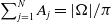 $\sum _{j=1}^{N} A_j={|\Omega |/\pi }$
. We then represent
$\sum _{j=1}^{N} A_j={|\Omega |/\pi }$
. We then represent
 $u$
in terms of the surface Neumann Green’s function and the volume average
$u$
in terms of the surface Neumann Green’s function and the volume average
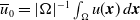 $\overline {u}_0=|\Omega |^{-1}\int _{\Omega } u({{\boldsymbol{x}}})\, d{{\boldsymbol{x}}}$
as
$\overline {u}_0=|\Omega |^{-1}\int _{\Omega } u({{\boldsymbol{x}}})\, d{{\boldsymbol{x}}}$
as
 \begin{equation} u({{\boldsymbol{x}}}) = \overline {u}_0 - \pi \sum \limits _{i=1}^N A_i G({{\boldsymbol{x}}},{{\boldsymbol{x}}}_i) . \end{equation}
Imposing the singularity behaviour in Eq. (3.20b), we obtain an
 $(N+1)$
-dimensional linear algebraic system for
$(N+1)$
-dimensional linear algebraic system for
 $\overline {u}_0$
and
$\overline {u}_0$
and
 $A_1,\ldots ,A_N$
given by
$A_1,\ldots ,A_N$
given by
 \begin{equation} A_j + \nu _j\left[A_j R_j + \sum \limits _{i=1 \atop i\ne j}^N G_{j,i} A_i\right] = \overline {u}_0 \nu _j, \quad j\in \lbrace {1,\ldots ,N\rbrace }; \qquad \sum _{j=1}^{N} A_j = \frac {|\Omega |}{\pi } , \end{equation}
where
 $G_{j,i}$
and
$G_{j,i}$
and
 $R_i$
were defined in (2.14). In matrix form Eq. (3.22) is written for
$R_i$
were defined in (2.14). In matrix form Eq. (3.22) is written for
 ${\textbf{A}}\equiv (A_1,\ldots ,A_N)^\dagger$
as
${\textbf{A}}\equiv (A_1,\ldots ,A_N)^\dagger$
as
 \begin{equation} {\textbf{A}} + {\boldsymbol \nu } {\textbf{G}} {\textbf{A}} = \overline {u}_0 {\boldsymbol \nu } {\textbf{e}} , \quad {\textbf{e}}^{T} {\textbf{A}} = \frac {|\Omega |}{\pi } , \end{equation}
where
 $\textbf{e}$
,
$\textbf{e}$
,
 $\boldsymbol \nu$
and the Green’s matrix
$\boldsymbol \nu$
and the Green’s matrix
 $\textbf{G}$
were defined in Eq. (2.15). By eliminating
$\textbf{G}$
were defined in Eq. (2.15). By eliminating
 $\overline {u}_0$
in Eq. (3.23), we conclude that
$\overline {u}_0$
in Eq. (3.23), we conclude that
 \begin{equation} \overline {u}_0 = \frac {|\Omega |}{\pi \bar {\nu }} + \frac {{\textbf{e}}^\dagger {\boldsymbol \nu } {\textbf{G}} {\textbf{A}}}{\bar {\nu }} , \end{equation}
where
 $\bar {\nu }\equiv \sum \limits _{j=1}^N \nu _j$
, while
$\bar {\nu }\equiv \sum \limits _{j=1}^N \nu _j$
, while
 $\textbf{A}$
is the solution to
$\textbf{A}$
is the solution to
 \begin{equation} {\textbf{M}}_0 {\textbf{A}} = \frac {|\Omega |}{\pi \bar {\nu }} {\boldsymbol \nu } , \end{equation}
with
 ${\textbf{M}}_0$
and
${\textbf{M}}_0$
and
 $\textbf{E}$
being defined in Eq. (2.20).
$\textbf{E}$
being defined in Eq. (2.20).
By using Eq. (3.12) for
 $\nu _j$
, which involves the local reactivity parameter
$\nu _j$
, which involves the local reactivity parameter
 $q_j$
on the patch, one can invert
$q_j$
on the patch, one can invert
 ${\textbf{M}}_0$
in Eq. (3.25) to get the coefficients
${\textbf{M}}_0$
in Eq. (3.25) to get the coefficients
 $A_j$
. As a consequence, Eq. (3.24) gives access to the volume-averaged MFRT
$A_j$
. As a consequence, Eq. (3.24) gives access to the volume-averaged MFRT
 $\overline {u}_0$
, whereas Eq. (3.21) determines the MFRT
$\overline {u}_0$
, whereas Eq. (3.21) determines the MFRT
 $u({{\boldsymbol{x}}})$
for any well-separated spatial configuration of partially reactive patches. This result generalises that in [Reference Pillay, Ward, Peirce and Kolokolnikov65], where perfect reactivities (
$u({{\boldsymbol{x}}})$
for any well-separated spatial configuration of partially reactive patches. This result generalises that in [Reference Pillay, Ward, Peirce and Kolokolnikov65], where perfect reactivities (
 $q_j=\infty$
) were assumed.
$q_j=\infty$
) were assumed.
4. Steklov-Neumann problem
As discussed in Section 1, the Robin boundary condition describes targets with a constant reactivity. In turn, more sophisticated surface reactions can be incorporated by using the encounter-based approach [Reference Grebenkov33, Reference Grebenkov34, Reference Grebenkov36], which relies on the mixed Steklov-Neumann problem. In this section, we apply the tools described above to derive the asymptotic properties of this spectral problem in the small-target limit.
As before, we consider a bounded planar domain
 $\Omega$
with a smooth boundary
$\Omega$
with a smooth boundary
 $\partial \Omega$
, which has
$\partial \Omega$
, which has
 $N$
small well-separated patches
$N$
small well-separated patches
 $\Gamma _{\varepsilon _j}$
, and
$\Gamma _{\varepsilon _j}$
, and
 $\partial \Omega _0 = \partial \Omega \backslash (\Gamma _{\varepsilon _1} \cup \ldots \cup \Gamma _{\varepsilon _N})$
. We study the mixed Steklov-Neumann spectral problem:
$\partial \Omega _0 = \partial \Omega \backslash (\Gamma _{\varepsilon _1} \cup \ldots \cup \Gamma _{\varepsilon _N})$
. We study the mixed Steklov-Neumann spectral problem:
 \begin{align} \Delta V & = 0 \quad \textrm {in}\,\Omega , \\[-12pt] \nonumber\end{align}
 \begin{align} \partial _n V & = \sigma V \quad \textrm {on}\, \Gamma _{\varepsilon _1} \cup \cdots \cup \Gamma _{\varepsilon _N} , \\[-12pt] \nonumber \end{align}
 \begin{align} \partial _n V & = 0 \quad \textrm {on} \, \partial \Omega _0 . \\[8pt] \nonumber \end{align}
This spectral problem is known to have a discrete positive spectrum [Reference Levitin, Mangoubi and Polterovich56], i.e., infinitely many eigenpairs
 $\{\sigma _k, V_k\}$
that are enumerated by
$\{\sigma _k, V_k\}$
that are enumerated by
 $k = 0,1,\ldots$
to form an increasing sequence of eigenvalues:
$k = 0,1,\ldots$
to form an increasing sequence of eigenvalues:
 $0 = \sigma _0 \lt \sigma _1 \leq \sigma _2 \leq \ldots \nearrow \infty$
. Note that the Steklov boundary condition (4.1b) with a nonnegative
$0 = \sigma _0 \lt \sigma _1 \leq \sigma _2 \leq \ldots \nearrow \infty$
. Note that the Steklov boundary condition (4.1b) with a nonnegative
 $\sigma$
differs from the previous Robin condition by the opposite sign. We aim at determining the asymptotic behaviour of the eigenvalues
$\sigma$
differs from the previous Robin condition by the opposite sign. We aim at determining the asymptotic behaviour of the eigenvalues
 $\sigma _k$
and the associated eigenfunctions
$\sigma _k$
and the associated eigenfunctions
 $V_k$
in the small-target limit.
$V_k$
in the small-target limit.
In the case of a single Steklov patch (
 $N = 1$
), the small-
$N = 1$
), the small-
 $\varepsilon _1$
asymptotic behaviour of the eigenvalues and eigenfunctions was analysed in [Reference Grebenkov38]. In fact, a simple scaling argument suggests that
$\varepsilon _1$
asymptotic behaviour of the eigenvalues and eigenfunctions was analysed in [Reference Grebenkov38]. In fact, a simple scaling argument suggests that
 $\sigma _j \approx \mu _j/\varepsilon _1$
(
$\sigma _j \approx \mu _j/\varepsilon _1$
(
 $j=1,2,\ldots$
) to leading order, where
$j=1,2,\ldots$
) to leading order, where
 $\mu _j$
are the eigenvalues of the mixed Steklov-Neumann problem (3.5) for the interval in the upper-half-plane (see also Appendix C).
$\mu _j$
are the eigenvalues of the mixed Steklov-Neumann problem (3.5) for the interval in the upper-half-plane (see also Appendix C).
If there are two well-separated Steklov patches, it is tempting to apply the same scaling argument in the vicinity of each patch. In this way, we can expect that the spectrum of the problem (4.1) with
 $N = 2$
is composed of two sequences of eigenvalues:
$N = 2$
is composed of two sequences of eigenvalues:
 $\{\mu _j/\varepsilon _1\}$
from the first patch of length
$\{\mu _j/\varepsilon _1\}$
from the first patch of length
 $2\varepsilon _1$
, and
$2\varepsilon _1$
, and
 $\{\mu _j/\varepsilon _2\}$
from the second patch of length
$\{\mu _j/\varepsilon _2\}$
from the second patch of length
 $2\varepsilon _2$
. In other words, the two patches might be expected to not interact with each other in the small-target limit as
$2\varepsilon _2$
. In other words, the two patches might be expected to not interact with each other in the small-target limit as
 $\varepsilon _j \to 0$
. This intuitive argument turns out to be correct for all the eigenvalues, except for the first nontrivial eigenvalue
$\varepsilon _j \to 0$
. This intuitive argument turns out to be correct for all the eigenvalues, except for the first nontrivial eigenvalue
 $\sigma _1$
. Indeed, if two patches could be treated as independent, the eigenvalue
$\sigma _1$
. Indeed, if two patches could be treated as independent, the eigenvalue
 $\sigma _1$
would have to be zero, as
$\sigma _1$
would have to be zero, as
 $\sigma _0$
. However, the zero eigenvalue can only correspond to a constant eigenfunction, so that if
$\sigma _0$
. However, the zero eigenvalue can only correspond to a constant eigenfunction, so that if
 $\sigma _1$
was zero, one would have
$\sigma _1$
was zero, one would have
 $V_1 = const = V_0$
, which is impossible. We conclude that even if the patches are extremely small, the eigenvalue
$V_1 = const = V_0$
, which is impossible. We conclude that even if the patches are extremely small, the eigenvalue
 $\sigma _1$
must be strictly positive, and its asymptotic behaviour must result from long-range interactions between two patches.
$\sigma _1$
must be strictly positive, and its asymptotic behaviour must result from long-range interactions between two patches.
In this section, we adapt the analysis from Section 3 to the case of
 $N$
Steklov patches and determine the asymptotic behaviour of the first
$N$
Steklov patches and determine the asymptotic behaviour of the first
 $N-1$
eigenvalues
$N-1$
eigenvalues
 $\sigma _j$
, for
$\sigma _j$
, for
 $j \in \lbrace {1,\ldots ,N-1\rbrace }$
, in this setting.
$j \in \lbrace {1,\ldots ,N-1\rbrace }$
, in this setting.
4.1. Matched asymptotic analysis
As before, we look at the inner solution near each Steklov patch
 $\Gamma _{\varepsilon _j}$
. Upon comparing the Robin and Steklov conditions (3.1, 4.1b), we notice two differences: (i)
$\Gamma _{\varepsilon _j}$
. Upon comparing the Robin and Steklov conditions (3.1, 4.1b), we notice two differences: (i)
 $q_j$
is replaced by
$q_j$
is replaced by
 $-\sigma$
, and (ii) there is no inhomogeneous term
$-\sigma$
, and (ii) there is no inhomogeneous term
 $q_j \delta _{j,k}$
in the right-hand side. Apart from these two points, the BVPs for
$q_j \delta _{j,k}$
in the right-hand side. Apart from these two points, the BVPs for
 $S_k({{\boldsymbol{x}}})$
and
$S_k({{\boldsymbol{x}}})$
and
 $V({{\boldsymbol{x}}})$
are identical. As a consequence, we can immediately rewrite the asymptotic behaviour (3.11) for each
$V({{\boldsymbol{x}}})$
are identical. As a consequence, we can immediately rewrite the asymptotic behaviour (3.11) for each
 $j\in \lbrace {1,\ldots ,N\rbrace }$
as
$j\in \lbrace {1,\ldots ,N\rbrace }$
as
 \begin{equation} V \sim A_j \left[\ln |{{\boldsymbol{x}}}-{{\boldsymbol{x}}}_j| + 1/\nu _j + {\mathcal{C}}({-}\sigma \varepsilon _j) + o(1) \right] \quad \textrm {as}\, {{\boldsymbol{x}}}\to {{\boldsymbol{x}}}_j, \end{equation}
where we now redefine
 $\nu _j$
as
$\nu _j$
as
 \begin{equation} \nu _j = - {1/\ln (\varepsilon _j)} , \end{equation}
and where
 $A_j$
is an unknown coefficient. Note that the constant term
$A_j$
is an unknown coefficient. Note that the constant term
 ${\mathcal{C}}({-}\sigma \varepsilon _j)$
is not incorporated into the new definition of
${\mathcal{C}}({-}\sigma \varepsilon _j)$
is not incorporated into the new definition of
 $\nu _j$
, as we did earlier in the Robin case.
$\nu _j$
, as we did earlier in the Robin case.
As before, the outer solution is represented as
 \begin{equation} V = \chi - \pi \sum \limits _{i=1}^N A_i G({{\boldsymbol{x}}},{{\boldsymbol{x}}}_i), \end{equation}
with an unknown constant
 $\chi$
. The divergence theorem still ensures the compatibility condition (2.11). Upon enforcing the singularity behaviour (4.2) for the solution in Eq. (4.4), we get
$\chi$
. The divergence theorem still ensures the compatibility condition (2.11). Upon enforcing the singularity behaviour (4.2) for the solution in Eq. (4.4), we get
 \begin{equation} \chi - ({\textbf{G}} {\textbf{A}})_j = A_j (1/\nu _j + {\mathcal{C}}({-}\sigma \varepsilon _j)), \quad j\in \lbrace {1,\ldots ,N\rbrace } , \end{equation}
where we used the matrix notations introduced in Eq. (2.15) of Section 2.3. Multiplying this equation by
 $\nu _j$
and introducing the diagonal matrix
$\nu _j$
and introducing the diagonal matrix
 $\textbf{C}$
formed by
$\textbf{C}$
formed by
 $\{{\mathcal{C}}({-}\sigma \varepsilon _1), \ldots , {\mathcal{C}}({-}\sigma \varepsilon _N)\}$
, we rewrite Eq. (4.5) as
$\{{\mathcal{C}}({-}\sigma \varepsilon _1), \ldots , {\mathcal{C}}({-}\sigma \varepsilon _N)\}$
, we rewrite Eq. (4.5) as
 \begin{equation} \bigl ({\textbf{I}} + {\boldsymbol \nu } {\textbf{G}} + {\boldsymbol \nu } {\textbf{C}}\bigr ) {\textbf{A}} = \chi {\boldsymbol \nu } {\textbf{e}} . \end{equation}
Left-multiplying this equation by
 ${\textbf{e}}^\dagger$
, and using
${\textbf{e}}^\dagger$
, and using
 ${\textbf{e}}^\dagger {\textbf{A}} = 0$
, we isolate
${\textbf{e}}^\dagger {\textbf{A}} = 0$
, we isolate
 $\chi$
as
$\chi$
as
 \begin{equation} \chi = \frac {1}{\bar {\nu }} \bigl ({\textbf{e}}^\dagger {\boldsymbol \nu }{\textbf{G}} + {\textbf{e}}^\dagger {\boldsymbol \nu }{\textbf{C}}\bigr ){\textbf{A}} , \end{equation}
where
 $\bar {\nu }$
was defined by Eq. (2.18). Substituting this expression back into Eq. (4.6), we obtain that
$\bar {\nu }$
was defined by Eq. (2.18). Substituting this expression back into Eq. (4.6), we obtain that
 \begin{equation} \biggl ({\textbf{I}} + \biggl ({\textbf{I}} - \frac {{\boldsymbol \nu } {\textbf{E}}}{\bar {\nu }}\biggr ) {\boldsymbol \nu } \left ( {\textbf{G}} + {\textbf{C}}\right ) \biggr ) {\textbf{A}} = \boldsymbol{0} . \end{equation}
The necessary and sufficient condition for the existence of a nontrivial solution to this matrix equation is
 \begin{equation} {\mathrm{det}}\biggl ({\textbf{I}} + \biggl ({\textbf{I}} - \frac {{\boldsymbol \nu } {\textbf{E}}}{\bar {\nu }}\biggr ) {\boldsymbol \nu } ({\textbf{G}} + {\textbf{C}})\biggr ) = \boldsymbol{0} . \end{equation}
The matrices
 $\boldsymbol \nu$
and
$\boldsymbol \nu$
and
 $\textbf{G}$
are determined by the sizes and arrangement of the Steklov patches, while the matrix
$\textbf{G}$
are determined by the sizes and arrangement of the Steklov patches, while the matrix
 $\textbf{C}$
is formed by
$\textbf{C}$
is formed by
 $\{{\mathcal{C}}({-}\sigma \varepsilon _1),\ldots , {\mathcal{C}}({-}\sigma \varepsilon _N)\}$
, with the function
$\{{\mathcal{C}}({-}\sigma \varepsilon _1),\ldots , {\mathcal{C}}({-}\sigma \varepsilon _N)\}$
, with the function
 ${\mathcal{C}}(\mu )$
given by Eq. (3.7). As a consequence, Eq. (4.9) determines the unknown parameter
${\mathcal{C}}(\mu )$
given by Eq. (3.7). As a consequence, Eq. (4.9) determines the unknown parameter
 $\sigma$
. Moreover, the functional form (3.7) implies that there are infinitely many negative solutions, denoted as
$\sigma$
. Moreover, the functional form (3.7) implies that there are infinitely many negative solutions, denoted as
 $-\sigma _j$
, which are actually small-target approximations of the Steklov eigenvalues.
$-\sigma _j$
, which are actually small-target approximations of the Steklov eigenvalues.
Let us first provide qualitative insights on these solutions. If the matrix
 $\textbf{C}$
was fixed in the small-target limit, the condition
$\textbf{C}$
was fixed in the small-target limit, the condition
 $\nu _j\ll 1$
would imply the smallness of the second matrix term in Eq. (4.9) as compared to the identity matrix
$\nu _j\ll 1$
would imply the smallness of the second matrix term in Eq. (4.9) as compared to the identity matrix
 $\textbf{I}$
, thus ensuring the positivity of the determinant. To compensate the smallness of the matrix
$\textbf{I}$
, thus ensuring the positivity of the determinant. To compensate the smallness of the matrix
 $\boldsymbol \nu$
, the matrix
$\boldsymbol \nu$
, the matrix
 $\textbf{C}$
must therefore be large in the small-target limit. This is possible when at least one
$\textbf{C}$
must therefore be large in the small-target limit. This is possible when at least one
 $\sigma \varepsilon _i$
is close to
$\sigma \varepsilon _i$
is close to
 $- \mu _{2k}$
for some
$- \mu _{2k}$
for some
 $k$
. In other words, one can expect that a solution
$k$
. In other words, one can expect that a solution
 $-\sigma _j$
of Eq. (4.9) is close to
$-\sigma _j$
of Eq. (4.9) is close to
 $\mu _{2k}/\varepsilon _i$
for some
$\mu _{2k}/\varepsilon _i$
for some
 $i$
and
$i$
and
 $k$
. This intuitive picture suggests that an eigenvalue
$k$
. This intuitive picture suggests that an eigenvalue
 $\sigma _j$
of the mixed Steklov-Neumann problem with
$\sigma _j$
of the mixed Steklov-Neumann problem with
 $N$
patches can be approximated by that on a single patch (say,
$N$
patches can be approximated by that on a single patch (say,
 $\Gamma _{\varepsilon _i}$
), as if there were no other patches and the associated eigenfunction was localised on
$\Gamma _{\varepsilon _i}$
), as if there were no other patches and the associated eigenfunction was localised on
 $\Gamma _{\varepsilon _i}$
. The situation is, however, more subtle in the vicinity of
$\Gamma _{\varepsilon _i}$
. The situation is, however, more subtle in the vicinity of
 $\mu _0 = 0$
. In the analysis below, we focus on the asymptotic behaviour of the first
$\mu _0 = 0$
. In the analysis below, we focus on the asymptotic behaviour of the first
 $N$
eigenvalues
$N$
eigenvalues
 $\sigma _j$
.
$\sigma _j$
.
4.2. First
 $N$
eigenvalues
$N$
eigenvalues

Let us assume that
 $- \mu = \sigma \varepsilon _j \ll 1$
for all
$- \mu = \sigma \varepsilon _j \ll 1$
for all
 $j = 1,\ldots ,N$
, so that we can apply the approximate relation (3.10) for the function
$j = 1,\ldots ,N$
, so that we can apply the approximate relation (3.10) for the function
 ${\mathcal{C}}(\mu )$
. Introducing the diagonal matrix
${\mathcal{C}}(\mu )$
. Introducing the diagonal matrix
 $\boldsymbol \eta$
formed by
$\boldsymbol \eta$
formed by
 $\{ {\pi /(2\varepsilon _1)}, \ldots , {\pi /(2\varepsilon _N)}\}$
, we get
$\{ {\pi /(2\varepsilon _1)}, \ldots , {\pi /(2\varepsilon _N)}\}$
, we get
 ${\textbf{C}} \approx - {\boldsymbol \eta }/\sigma + C_1 {\textbf{I}}$
. Its substitution into Eq. (4.9) yields
${\textbf{C}} \approx - {\boldsymbol \eta }/\sigma + C_1 {\textbf{I}}$
. Its substitution into Eq. (4.9) yields
 \begin{equation} {\mathrm{det}}\biggl ({\textbf{I}} + \biggl ({\textbf{I}} - \frac {{\boldsymbol \nu } {\textbf{E}}}{\bar {\nu }}\biggr ) {\boldsymbol \nu } \bigl [{\textbf{G}} - {\boldsymbol \eta }/\sigma + C_1 {\textbf{I}}\bigr ]\biggr ) = \boldsymbol{0} . \end{equation}
Upon defining
 ${\textbf{M}}_1$
and
${\textbf{M}}_1$
and
 ${\textbf{B}}_1$
by
${\textbf{B}}_1$
by
 \begin{equation} {\textbf{M}}_1 = {\textbf{I}} + \biggl ({\textbf{I}} - \frac {{\boldsymbol \nu } {\textbf{E}}}{\bar {\nu }}\biggr ) {\boldsymbol \nu } \bigl ({\textbf{G}} + C_1 {\textbf{I}}\bigr ) , \qquad {\textbf{B}}_1 = \biggl ({\textbf{I}} - \frac {{\boldsymbol \nu } {\textbf{E}}}{\bar {\nu }}\biggr ) {\boldsymbol \nu } {\boldsymbol \eta }, \end{equation}
we can rewrite Eq. (4.10) in a more compact form as
 \begin{equation} {\mathrm{det}}(\sigma {\textbf{M}}_1 - {\textbf{B}}_1) = 0. \end{equation}
In the small-target limit, one has
 $\nu _j \ll 1$
so that
$\nu _j \ll 1$
so that
 ${\textbf{M}}_1$
is invertible since it is a small perturbation of the identity matrix. As a consequence, we get that
${\textbf{M}}_1$
is invertible since it is a small perturbation of the identity matrix. As a consequence, we get that
 \begin{equation} {\mathrm{det}}(\sigma {\textbf{I}} - {\textbf{M}}_1^{-1} {\textbf{B}}_1) = 0. \end{equation}
We now prove that the eigenvalues
 $\hat {\sigma }_j$
for
$\hat {\sigma }_j$
for
 $j=0,\ldots ,N-1$
of the matrix
$j=0,\ldots ,N-1$
of the matrix
 ${\textbf{M}}_1^{-1} {\textbf{B}}_1$
are real. To do so, we first write
${\textbf{M}}_1^{-1} {\textbf{B}}_1$
are real. To do so, we first write
 ${\textbf{M}}_1$
in Eq. (4.11) as
${\textbf{M}}_1$
in Eq. (4.11) as
 \begin{equation} {\textbf{M}}_1 = {\textbf{I}} - \hat {{\textbf{B}}}_1 \hat {{\textbf{G}}} , \,\, \end{equation}
where we define the symmetric matrices
 $\hat {{\textbf{B}}}_1$
and
$\hat {{\textbf{B}}}_1$
and
 $\hat {{\textbf{G}}}$
by
$\hat {{\textbf{G}}}$
by
 \begin{equation} \hat {{\textbf{B}}}_1={\textbf{B}}_1{\boldsymbol \eta }^{-1} = \left ({\textbf{I}} - \frac {{\boldsymbol \nu } {\textbf{E}}}{\bar {\nu }}\right ){\boldsymbol \nu } , \qquad \hat {{\textbf{G}}}=-{\textbf{G}} - C_1 {\textbf{I}} . \end{equation}
By using the Neumann series to calculate
 ${\textbf{M}}_1^{-1}$
, which converges since
${\textbf{M}}_1^{-1}$
, which converges since
 $\nu _j\ll 1$
, we obtain that
$\nu _j\ll 1$
, we obtain that
 \begin{equation} {\textbf{M}}_1^{-1} \hat {{\textbf{B}}}_1 = \hat {{\textbf{B}}}_1 + \hat {{\textbf{B}}}_1\left (\sum _{n=1}^{\infty } {\textbf{K}}_n\right ) \hat {{\textbf{B}}}_1 , \qquad {\textbf{K}}_n = \left ( \hat {{\textbf{G}}} \hat {{\textbf{B}}}_1\right )^{n-1} \hat {{\textbf{G}}} . \end{equation}
Since
 ${\textbf{K}}_n$
is symmetric for each
${\textbf{K}}_n$
is symmetric for each
 $n=1,2,\ldots$
, it follows that
$n=1,2,\ldots$
, it follows that
 ${\textbf{M}}_1^{-1}\hat {{\textbf{B}}}_1$
is symmetric. Finally, we denote
${\textbf{M}}_1^{-1}\hat {{\textbf{B}}}_1$
is symmetric. Finally, we denote
 ${\textbf{D}}={\textbf{M}}_1^{-1}{\textbf{B}}_1 ={\textbf{M}}_{1}^{-1}\hat {{\textbf{B}}}_1 {\boldsymbol \eta }$
and introduce
${\textbf{D}}={\textbf{M}}_1^{-1}{\textbf{B}}_1 ={\textbf{M}}_{1}^{-1}\hat {{\textbf{B}}}_1 {\boldsymbol \eta }$
and introduce
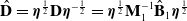 $\hat {{\textbf{D}}} = {\boldsymbol \eta }^{\frac 12} {\textbf{D}} {\boldsymbol \eta }^{-\frac 12} = {\boldsymbol \eta }^{\frac 12} {\textbf{M}}_1^{-1} \hat {{\textbf{B}}}_1 {\boldsymbol \eta }^{\frac 12}$
, which is symmetric, so that its eigenvalues are real. Since
$\hat {{\textbf{D}}} = {\boldsymbol \eta }^{\frac 12} {\textbf{D}} {\boldsymbol \eta }^{-\frac 12} = {\boldsymbol \eta }^{\frac 12} {\textbf{M}}_1^{-1} \hat {{\textbf{B}}}_1 {\boldsymbol \eta }^{\frac 12}$
, which is symmetric, so that its eigenvalues are real. Since
 $\boldsymbol \eta$
is positive definite,
$\boldsymbol \eta$
is positive definite,
 $\hat {{\textbf{D}}}$
is related to
$\hat {{\textbf{D}}}$
is related to
 $\textbf{D}$
by a similarity transformation so that the latter must also have real eigenvalues
$\textbf{D}$
by a similarity transformation so that the latter must also have real eigenvalues
 $\hat {\sigma }_j$
for
$\hat {\sigma }_j$
for
 $j=0,\ldots ,N-1$
.
$j=0,\ldots ,N-1$
.
Moreover, we note that
 $\hat {\sigma }_0 = 0$
. This follows since
$\hat {\sigma }_0 = 0$
. This follows since
 ${\textbf{B}}_1^\dagger {\textbf{e}} = 0$
, so that
${\textbf{B}}_1^\dagger {\textbf{e}} = 0$
, so that
 $\textbf{e}$
is an eigenvector of
$\textbf{e}$
is an eigenvector of
 ${\textbf{B}}_1^\dagger$
and thus of
${\textbf{B}}_1^\dagger$
and thus of
 $[{\textbf{M}}_1^\dagger ]^{-1} {\textbf{B}}_1^\dagger$
. The associated eigenvalue
$[{\textbf{M}}_1^\dagger ]^{-1} {\textbf{B}}_1^\dagger$
. The associated eigenvalue
 $0$
is thus an eigenvalue of
$0$
is thus an eigenvalue of
 ${\textbf{B}}_1 {\textbf{M}}_1^{-1}$
as well as of
${\textbf{B}}_1 {\textbf{M}}_1^{-1}$
as well as of
 ${\textbf{M}}_1^{-1} {\textbf{B}}_1$
.
${\textbf{M}}_1^{-1} {\textbf{B}}_1$
.
In summary, the eigenvalues of the matrix
 ${\textbf{M}}_1^{-1} {\textbf{B}}_1$
provide the leading terms in the asymptotic behaviour of the first
${\textbf{M}}_1^{-1} {\textbf{B}}_1$
provide the leading terms in the asymptotic behaviour of the first
 $N$
eigenvalues
$N$
eigenvalues
 $\sigma _j$
of the Steklov-Neumann problem:
$\sigma _j$
of the Steklov-Neumann problem:
 \begin{equation} \sigma _j \approx \hat {\sigma }_j, \qquad j\in \lbrace {1,\ldots ,N-1\rbrace }. \end{equation}
This is the main result of this section. We observe that
 $\sigma _0 = \hat {\sigma }_0 = 0$
, as expected.
$\sigma _0 = \hat {\sigma }_0 = 0$
, as expected.
4.3. Associated eigenfunctions
In addition, we construct the associated eigenfunctions of the first
 $N$
eigenvalues. For this purpose, let us rewrite Eq. (4.8) as
$N$
eigenvalues. For this purpose, let us rewrite Eq. (4.8) as
 \begin{equation} (\sigma {\textbf{I}} - {\textbf{M}}_1^{-1} {\textbf{B}}_1) {\textbf{A}} = \boldsymbol{0}. \end{equation}
While each eigenvalue
 $\hat {\sigma }_j$
of the matrix
$\hat {\sigma }_j$
of the matrix
 ${\textbf{M}}_1^{-1} {\textbf{B}}_1$
approximates the
${\textbf{M}}_1^{-1} {\textbf{B}}_1$
approximates the
 $j$
-th eigenvalue of the mixed Steklov-Neumann problem, the corresponding eigenvector of this matrix is the vector of coefficients
$j$
-th eigenvalue of the mixed Steklov-Neumann problem, the corresponding eigenvector of this matrix is the vector of coefficients
 $A_i$
determining the associated eigenfunction
$A_i$
determining the associated eigenfunction
 $V_j$
via Eq. (4.4), up to a multiplicative factor; we recall that
$V_j$
via Eq. (4.4), up to a multiplicative factor; we recall that
 $\chi$
is given by Eq. (4.7).
$\chi$
is given by Eq. (4.7).
The missing multiplicative factor can be fixed by imposing an appropriate normalisation of eigenfunctions. For the Steklov problem, the natural normalisation is
 \begin{equation} \int \limits _{\Gamma } V^2\, ds = 1 , \end{equation}
where
 $\Gamma = \Gamma _{\varepsilon _1}\cup \cdots \cup \Gamma _{\varepsilon _N}$
. For the trivial eigenvalue
$\Gamma = \Gamma _{\varepsilon _1}\cup \cdots \cup \Gamma _{\varepsilon _N}$
. For the trivial eigenvalue
 $\sigma _0 = 0$
, one has a constant eigenfunction
$\sigma _0 = 0$
, one has a constant eigenfunction
 $V_0$
, whose normalisation yields:
$V_0$
, whose normalisation yields:
 $V_0^2 = 1/|\Gamma |$
. In the following, we assume that
$V_0^2 = 1/|\Gamma |$
. In the following, we assume that
 $\sigma \gt 0$
.
$\sigma \gt 0$
.
To proceed, we recall that the inner solution near the
 $i$
-th patch reads in local coordinates is
$i$
-th patch reads in local coordinates is
 \begin{equation} V({{\boldsymbol{x}}}_i + \varepsilon _i \textbf{Q}_i^\dagger {\boldsymbol{y}}) \approx A_i g_{-\sigma \varepsilon _i}(\,{\boldsymbol{y}}). \end{equation}
Using the representation (3.4) of the Green’s function
 $g_{\mu }(\,{\boldsymbol{y}})$
, the restriction of
$g_{\mu }(\,{\boldsymbol{y}})$
, the restriction of
 $V$
onto
$V$
onto
 $\Gamma _i$
becomes
$\Gamma _i$
becomes
 \begin{equation} V|_{\Gamma _i}(y_1) = V({{\boldsymbol{x}}}_i + \varepsilon _i \textbf{Q}_i^\dagger (y_1,0)^\dagger ) \approx \pi A_i \sum \limits _{k=0}^\infty \frac {\Psi _{2k}(\infty ) \Psi _{2k}(y_1,0)}{\mu _{2k} - \sigma \varepsilon _i} . \end{equation}
This equation helps to deduce the required condition on the coefficients
 $A_i$
:
$A_i$
:
 \begin{align*} 1 & = \sum \limits _{i=1}^N \int \limits _{\Gamma _i} V^2 \, ds = \sum \limits _{i=1}^N \varepsilon _i \pi ^2 A_i^2 \sum \limits _{k=0}^\infty \frac {[\Psi _{2k}(\infty )]^2}{(\mu _{2k} - \sigma \varepsilon _i)^2} , \end{align*}
where we used the orthogonality of the eigenfunctions
 $\Psi _k$
(see Appendix C). The last sum can be re-written as the derivative of
$\Psi _k$
(see Appendix C). The last sum can be re-written as the derivative of
 ${\mathcal{C}}(\mu )$
, denoted as
${\mathcal{C}}(\mu )$
, denoted as
 ${\mathcal{C}}^{\prime }(\mu )$
:
${\mathcal{C}}^{\prime }(\mu )$
:
 \begin{equation} 1 = - \pi \sum \limits _{i=1}^N \varepsilon _i A_i^2 {\mathcal{C}}^{\prime }({-}\sigma \varepsilon _i) . \end{equation}
When
 $0 \lt \sigma \varepsilon _i \ll 1$
, the Taylor expansion (3.8) implies
$0 \lt \sigma \varepsilon _i \ll 1$
, the Taylor expansion (3.8) implies
 ${\mathcal{C}}^{\prime }(\mu ) \approx -\pi /(2\mu ^2)$
and thus
${\mathcal{C}}^{\prime }(\mu ) \approx -\pi /(2\mu ^2)$
and thus
 \begin{equation} \frac {2\sigma ^2}{\pi ^2} \approx \sum \limits _{i=1}^N \frac {A_i^2}{\varepsilon _i } . \end{equation}
To complete this section, let us briefly discuss the positivity of Steklov eigenfunctions on patches
 $\Gamma _{\varepsilon _j}$
. For a single patch, all Steklov eigenfunctions
$\Gamma _{\varepsilon _j}$
. For a single patch, all Steklov eigenfunctions
 $V_j$
must change sign on the patch due to their orthogonality to
$V_j$
must change sign on the patch due to their orthogonality to
 $V_0 = 1/\sqrt {|\Gamma |}$
. When there are
$V_0 = 1/\sqrt {|\Gamma |}$
. When there are
 $N$
Steklov patches, the orthogonality still holds so that any eigenfunction
$N$
Steklov patches, the orthogonality still holds so that any eigenfunction
 $V_j$
with
$V_j$
with
 $j \gt 0$
must change sign on the union of patches
$j \gt 0$
must change sign on the union of patches
 $\Gamma = \Gamma _{\varepsilon _1} \cup \cdots \cup \Gamma _{\varepsilon _N}$
. However, it is generally unknown whether
$\Gamma = \Gamma _{\varepsilon _1} \cup \cdots \cup \Gamma _{\varepsilon _N}$
. However, it is generally unknown whether
 $V_j$
changes the sign or not on each patch
$V_j$
changes the sign or not on each patch
 $\Gamma _i$
. Looking at Eq. (4.21), one can expect that if
$\Gamma _i$
. Looking at Eq. (4.21), one can expect that if
 $\sigma \varepsilon _i$
is small enough, the eigenfunction
$\sigma \varepsilon _i$
is small enough, the eigenfunction
 $V$
does not change sign on the patch
$V$
does not change sign on the patch
 $\Gamma _i$
(i.e., it is either positive or negative on it). Indeed, the term
$\Gamma _i$
(i.e., it is either positive or negative on it). Indeed, the term
 $1/({-}2\sigma \varepsilon _i)$
of the sum in Eq. (4.21) that corresponds to
$1/({-}2\sigma \varepsilon _i)$
of the sum in Eq. (4.21) that corresponds to
 $k = 0$
, is expected to provide the dominant contribution as compared to the remaining terms. This property follows from the conjectured inequality (C.9). In other words, if the patches are small enough, the first
$k = 0$
, is expected to provide the dominant contribution as compared to the remaining terms. This property follows from the conjectured inequality (C.9). In other words, if the patches are small enough, the first
 $N$
eigenfunctions do not change their signs on each patch. This conjecture is confirmed by several numerical examples (not shown).
$N$
eigenfunctions do not change their signs on each patch. This conjecture is confirmed by several numerical examples (not shown).
4.4. Example of two patches
When
 $N = 2$
, we calculate that
$N = 2$
, we calculate that
 \begin{equation} ({\textbf{I}} - {\boldsymbol \nu } {\textbf{E}}/\bar {\nu }){\boldsymbol \nu } = \gamma \left (\begin{array}{c@{\quad}c} 1 & -1 \\ -1 & 1 \\ \end{array} \right ), \end{equation}
where we label
 $\gamma = \nu _1\nu _2/(\nu _1+ \nu _2)$
. Then, from Eq. (4.11), we get
$\gamma = \nu _1\nu _2/(\nu _1+ \nu _2)$
. Then, from Eq. (4.11), we get
 \begin{equation*} {\textbf{M}}_1 = {\textbf{I}} + \gamma \left (\begin{array}{c@{\quad}c} (R_1 - G_{1,2}) + C_1 & (G_{1,2} - R_2)-C_1 \\[4pt] (G_{1,2}-R_1) - C_1 & (R_2 - G_{1,2}) + C_1 \\ \end{array} \right ) , \qquad {\textbf{B}}_1 = \frac {\pi }{2} \gamma \left (\begin{array}{c@{\quad}c} 1/\varepsilon _1 & -1/\varepsilon _2 \\[4pt] -1/\varepsilon _1 & 1/\varepsilon _2 \\ \end{array} \right ). \end{equation*}
Since
 $\textbf{e}$
is a left-eigenvector of
$\textbf{e}$
is a left-eigenvector of
 ${\textbf{M}}_1$
with eigenvalue one, the second eigenvalue of
${\textbf{M}}_1$
with eigenvalue one, the second eigenvalue of
 ${\textbf{M}}_1$
is simply
${\textbf{M}}_1$
is simply
 $\mathrm{trace}({\textbf{M}}_1)-1$
. As a consequence, we find
$\mathrm{trace}({\textbf{M}}_1)-1$
. As a consequence, we find
 \begin{equation} {\mathrm{det}}({\textbf{M}}_1) = \mathrm{trace}({\textbf{M}}_1)-1=1 + \gamma [(R_1 + R_2 - 2G_{1,2}) + 2C_1] , \end{equation}
and
 \begin{equation} {\textbf{M}}_1^{-1} = \frac {1}{{\mathrm{det}}({\textbf{M}}_1)}\biggl [{\textbf{I}} + \gamma C_1 {\textbf{E}} + \gamma \left (\begin{array}{c@{\quad}c} R_2 - G_{1,2} & R_2-G_{1,2} \\[4pt] R_1 - G_{1,2} & R_1 - G_{1,2} \\ \end{array} \right )\biggr ] , \end{equation}
from which we calculate
 \begin{equation} {\textbf{M}}_1^{-1} {\textbf{B}}_1 = \frac {\pi \gamma /2}{{\mathrm{det}}({\textbf{M}}_1)} \left (\begin{array}{cc} 1/\varepsilon _1 & - 1/\varepsilon _2 \\[4pt] -1/\varepsilon _1 & 1/\varepsilon _2 \\ \end{array} \right ). \end{equation}
The two eigenvalues of this matrix are
 $\hat {\sigma }_0 = 0$
and
$\hat {\sigma }_0 = 0$
and
 \begin{equation} \hat {\sigma }_1 = \frac {\pi \gamma (1/\varepsilon _1 + 1/\varepsilon _2)}{2\,{\mathrm{det}}({\textbf{M}}_1)} , \end{equation}
so that upon solving for
 $\hat {\sigma }_1^{-1}$
, we get
$\hat {\sigma }_1^{-1}$
, we get
 \begin{equation} \frac {1}{\hat {\sigma }_1} = \frac {2\varepsilon _1\varepsilon _2}{\pi (\varepsilon _1+\varepsilon _2)} \biggl [\frac {1}{\gamma } + (R_1 + R_2 - 2G_{1,2}) + 2C_1\biggr ] . \end{equation}
To simplify this expression, we use
 \begin{equation} \gamma = \frac {1}{1/\nu _1 + 1/\nu _2} = \frac {1}{-\ln (\varepsilon _1\varepsilon _2)} . \end{equation}
This yields the following asymptotic behaviour for the Steklov eigenvalue:
 \begin{align} \frac {1}{\sigma _1} \approx \frac {2\varepsilon _1\varepsilon _2}{\pi (\varepsilon _1+\varepsilon _2)} [{-}\ln (\varepsilon _1\varepsilon _2) + 2C_1 + (R_1 + R_2 - 2G_{1,2})]. \end{align}
For instance, if
 $\Omega$
is the unit disk, Eq. (2.28) yields
$\Omega$
is the unit disk, Eq. (2.28) yields
 \begin{align} \frac {1}{\sigma _1} \approx \frac {2\varepsilon _1\varepsilon _2}{\pi (\varepsilon _1+\varepsilon _2)} ({-}\ln (\varepsilon _1\varepsilon _2) + 2C_1 + 2\ln |{{\boldsymbol{x}}}_1-{{\boldsymbol{x}}}_2|). \end{align}
Moreover, the corresponding eigenfunction
 $V_1$
can be easily found by noting that
$V_1$
can be easily found by noting that
 $A_1 = -A_2$
from Eq. (2.11), whereas Eq. (4.23) implies
$A_1 = -A_2$
from Eq. (2.11), whereas Eq. (4.23) implies
 \begin{equation} A_1 = -A_2 \approx \frac {\sqrt {2} \sigma _1}{\pi \sqrt {1/\varepsilon _1 + 1/\varepsilon _2}} . \end{equation}
These coefficients determine
 $(V_1)|_{\Gamma _i}$
via Eq. (4.21).
$(V_1)|_{\Gamma _i}$
via Eq. (4.21).
4.5. Example of identical equally spaced patches on the boundary of the unit disk
When all patches are of the same size,
 $\varepsilon _j = \varepsilon$
, we have
$\varepsilon _j = \varepsilon$
, we have
 ${\boldsymbol \nu } = \nu {\textbf{I}}$
and
${\boldsymbol \nu } = \nu {\textbf{I}}$
and
 ${\boldsymbol \eta } = {\textbf{I}} \pi /(2\varepsilon )$
, so that
${\boldsymbol \eta } = {\textbf{I}} \pi /(2\varepsilon )$
, so that
 \begin{equation} {\textbf{M}}_1 = {\textbf{I}} + \nu \biggl ({\textbf{I}} - \frac {{\textbf{E}}}{N}\biggr ) ({\textbf{G}} + C_1 {\textbf{I}}), \qquad {\textbf{B}}_1 = \frac {\pi \nu }{2\varepsilon } \biggl ({\textbf{I}} - \frac {{\textbf{E}}}{N}\biggr ) . \end{equation}
If the patches are equally spaced on the boundary of the unit disk,
 $\textbf{G}$
is circulant and symmetric, and its eigenvectors and eigenvalues were given in Eqs. (2.32, 2.33). As shown earlier in Section 2.5, one has
$\textbf{G}$
is circulant and symmetric, and its eigenvectors and eigenvalues were given in Eqs. (2.32, 2.33). As shown earlier in Section 2.5, one has
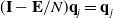 $({\textbf{I}} - {\textbf{E}}/N) \textbf{q}_j = \textbf{q}_j$
for any
$({\textbf{I}} - {\textbf{E}}/N) \textbf{q}_j = \textbf{q}_j$
for any
 $j = 1,2,\ldots ,N-1$
, and
$j = 1,2,\ldots ,N-1$
, and
 $({\textbf{I}} - {\textbf{E}}/N) \textbf{q}_N = 0$
. As a consequence,
$({\textbf{I}} - {\textbf{E}}/N) \textbf{q}_N = 0$
. As a consequence,
 ${\textbf{M}}_1 \textbf{q}_N = \textbf{q}_N$
and
${\textbf{M}}_1 \textbf{q}_N = \textbf{q}_N$
and
 ${\textbf{M}}_1 \textbf{q}_j = (1 + \nu (\kappa _j+C_1)) \textbf{q}_j$
, where
${\textbf{M}}_1 \textbf{q}_j = (1 + \nu (\kappa _j+C_1)) \textbf{q}_j$
, where
 $\kappa _j$
are given explicitly by Eq. (2.40). Upon calculating
$\kappa _j$
are given explicitly by Eq. (2.40). Upon calculating
 ${\textbf{M}}_1^{-1}\textbf{q}_j$
, we readily find that
${\textbf{M}}_1^{-1}\textbf{q}_j$
, we readily find that
 \begin{equation*} {\textbf{B}}_1 {\textbf{M}}_1^{-1} \textbf{q}_N = 0, \qquad {\textbf{B}}_1 {\textbf{M}}_1^{-1} \textbf{q}_j = \frac {\pi \nu }{2\varepsilon } \bigl (1 + \nu (\kappa _j+C_1)\bigr )^{-1} \textbf{q}_j . \end{equation*}
Since the eigenvalues of the matrices
 ${\textbf{B}}_1 {\textbf{M}}_1^{-1}$
and
${\textbf{B}}_1 {\textbf{M}}_1^{-1}$
and
 ${\textbf{M}}_1^{-1}{\textbf{B}}_1$
are identical, we have from Eq. (4.13) that
${\textbf{M}}_1^{-1}{\textbf{B}}_1$
are identical, we have from Eq. (4.13) that
 $\hat {\sigma }_0 = 0$
and
$\hat {\sigma }_0 = 0$
and
 \begin{equation} \hat {\sigma }_j = \frac {\pi \nu }{2\varepsilon [1 + \nu (\kappa _j+C_1)]}, \qquad j\in \lbrace {1,\ldots ,N-1\rbrace }. \end{equation}
Substituting
 $C_1={3/2}-\ln {2}$
from Eq. (3.9) and
$C_1={3/2}-\ln {2}$
from Eq. (3.9) and
 $\nu ={-1/\ln \varepsilon }$
into Eq. (4.35), we obtain the following small-
$\nu ={-1/\ln \varepsilon }$
into Eq. (4.35), we obtain the following small-
 $\varepsilon$
asymptotic result for the first
$\varepsilon$
asymptotic result for the first
 $N-1$
eigenvalues of the mixed Steklov-Neumann problem:
$N-1$
eigenvalues of the mixed Steklov-Neumann problem:
 \begin{equation} \frac {1}{\varepsilon \sigma _j} \approx \frac {2}{\pi } \biggl ({-}\ln (\varepsilon ) + \frac 32 - \ln (2) + \kappa _j \biggr ), \end{equation}
for
 $j = 1,2,\ldots ,N-1$
. When the number of patches is large, i.e.
$j = 1,2,\ldots ,N-1$
. When the number of patches is large, i.e.
 $N \gg 1$
, while still enforcing the well-separated patch assumption
$N \gg 1$
, while still enforcing the well-separated patch assumption
 $\varepsilon N\ll \pi$
, we can use the asymptotic relation (B.12) for
$\varepsilon N\ll \pi$
, we can use the asymptotic relation (B.12) for
 $\kappa _j$
, valid for
$\kappa _j$
, valid for
 $j\ll N$
, to conclude that
$j\ll N$
, to conclude that
 \begin{equation} \frac {1}{\varepsilon \sigma _j} \approx \frac {2}{\pi } \biggl ( \frac {N}{2j} -\ln \left (\frac {N\varepsilon }{\pi }\right ) - \frac {1}{3}\biggr ). \end{equation}
If
 $N\varepsilon$
is not too small, the logarithmic and constant terms can be neglected to yield to a first approximation
$N\varepsilon$
is not too small, the logarithmic and constant terms can be neglected to yield to a first approximation
 \begin{equation} \sigma _j \approx \frac {\pi j}{N\varepsilon } \quad \mbox{for} \quad j\ll N, \end{equation}
when
 $N\gg 1$
. It is instructive to compare this approximation to the case of a single Steklov patch of half-length
$N\gg 1$
. It is instructive to compare this approximation to the case of a single Steklov patch of half-length
 $\varepsilon _1 = N\varepsilon$
, for which
$\varepsilon _1 = N\varepsilon$
, for which
 $\sigma _j \approx \mu _j/\varepsilon _1 \approx (\pi j/2)/(N\varepsilon )$
, where we used the asymptotic relation (C.11). As a consequence, the configuration with a single patch of half-length
$\sigma _j \approx \mu _j/\varepsilon _1 \approx (\pi j/2)/(N\varepsilon )$
, where we used the asymptotic relation (C.11). As a consequence, the configuration with a single patch of half-length
 $N\varepsilon$
yields approximately twice smaller eigenvalues. This suggests that the fragmentation of a patch will increase the eigenvalues.
$N\varepsilon$
yields approximately twice smaller eigenvalues. This suggests that the fragmentation of a patch will increase the eigenvalues.
5. Steklov-Neumann-Dirichlet problem
In this section, we consider the last setting of a single Steklov patch
 $\Gamma _{\varepsilon _1}$
and
$\Gamma _{\varepsilon _1}$
and
 $N-1$
Dirichlet patches
$N-1$
Dirichlet patches
 $\Gamma _{\varepsilon _j}$
(
$\Gamma _{\varepsilon _j}$
(
 $j = 2,\ldots ,N$
). This is a typical situation when the diffusing particle needs to react on
$j = 2,\ldots ,N$
). This is a typical situation when the diffusing particle needs to react on
 $\Gamma _{\varepsilon _1}$
before escaping the domain
$\Gamma _{\varepsilon _1}$
before escaping the domain
 $\Omega$
through multiple opening windows
$\Omega$
through multiple opening windows
 $\Gamma _{\varepsilon _2}, \ldots , \Gamma _{\varepsilon _N}$
. A formal solution of such an escape problem was provided in [Reference Grebenkov37] on the basis of the mixed Steklov-Neumann-Dirichlet spectral problem, formulated as
$\Gamma _{\varepsilon _2}, \ldots , \Gamma _{\varepsilon _N}$
. A formal solution of such an escape problem was provided in [Reference Grebenkov37] on the basis of the mixed Steklov-Neumann-Dirichlet spectral problem, formulated as
 \begin{align} \Delta V & = 0 \quad \textrm {in}\,\Omega , \\[-6pt] \nonumber \end{align}
 \begin{align} \partial _n V & = \sigma V \quad \textrm {on}\, \Gamma _{\varepsilon _1} ; \qquad V = 0 \quad \textrm {on} \, \Gamma _{\varepsilon _2} \cup \cdots \cup \Gamma _{\varepsilon _N} , \\[-6pt] \nonumber \end{align}
 \begin{align} \partial _n V & = 0 \quad \textrm {on} \, \partial \Omega _0 .\\[8pt] \nonumber \end{align}
As previously, this spectral problem is known to have a discrete positive spectrum [Reference Levitin, Mangoubi and Polterovich56], i.e., infinitely many eigenpairs
 $\{\sigma _k, V_k\}$
that are enumerated by
$\{\sigma _k, V_k\}$
that are enumerated by
 $k = 0,1,\ldots$
to form an increasing sequence of eigenvalues:
$k = 0,1,\ldots$
to form an increasing sequence of eigenvalues:
 $0 \lt \sigma _0 \leq \sigma _1 \leq \ldots \nearrow \infty$
. The presence of Dirichlet patches implies that the principal eigenvalue
$0 \lt \sigma _0 \leq \sigma _1 \leq \ldots \nearrow \infty$
. The presence of Dirichlet patches implies that the principal eigenvalue
 $\sigma _0$
is strictly positive. We aim at determining the asymptotic behaviour of the eigenvalues and eigenfunctions of this spectral problem in the small-target limit
$\sigma _0$
is strictly positive. We aim at determining the asymptotic behaviour of the eigenvalues and eigenfunctions of this spectral problem in the small-target limit
 $\varepsilon _j\to 0$
.
$\varepsilon _j\to 0$
.
In the analysis below, we treat separately two cases depending on the integral of the Steklov eigenfunction on the Steklov patch
 $\Gamma _{\varepsilon _1}$
. In particular, if
$\Gamma _{\varepsilon _1}$
. In particular, if
 \begin{equation} \int _{\Gamma _{\varepsilon _1}} \partial _n V \, ds = \sigma \int _{\Gamma _{\varepsilon _1}} V \, ds \ne 0, \end{equation}
then, from the divergence theorem, the Steklov patch produces a logarithmic contribution to the far field. We will mainly focus on this generic case. However, if the integral in Eq. (5.2) is zero (e.g., if
 $V|_{\Gamma _{\varepsilon _1}}$
is antisymmetric, see below), there is no logarithmic contribution, and such an eigenfunction vanishes in the far field. This situation is actually simpler because the decay of
$V|_{\Gamma _{\varepsilon _1}}$
is antisymmetric, see below), there is no logarithmic contribution, and such an eigenfunction vanishes in the far field. This situation is actually simpler because the decay of
 $V$
away from the Steklov patch is compatible with Dirichlet patches. In other words, we can restrict the analysis to the inner solution near the Steklov patch as if there were no Dirichlet patches. We will illustrate this situation in Section 5.4.
$V$
away from the Steklov patch is compatible with Dirichlet patches. In other words, we can restrict the analysis to the inner solution near the Steklov patch as if there were no Dirichlet patches. We will illustrate this situation in Section 5.4.
5.1. Matched asymptotic analysis
Expectedly, we can combine formerly derived inner solutions for Dirichlet and Steklov patches, whereas the outer solution is still written as the linear combination (4.4). As a consequence, we must enforce the singularity behaviour
 \begin{equation} V \sim A_j \left[\ln |{{\boldsymbol{x}}}-{{\boldsymbol{x}}}_j| + 1/\nu _j + \delta _{j,1} {\mathcal{C}}({-}\sigma \varepsilon _1) + o(1)\right] , \end{equation}
as
 ${{\boldsymbol{x}}}\to {{\boldsymbol{x}}}_j$
for all patches
${{\boldsymbol{x}}}\to {{\boldsymbol{x}}}_j$
for all patches
 $j\in \lbrace {1,\ldots ,N\rbrace }$
. Here, we have used the former definition
$j\in \lbrace {1,\ldots ,N\rbrace }$
. Here, we have used the former definition
 $\nu _j = -1/\ln (\varepsilon _j/2)$
for Dirichlet patches and
$\nu _j = -1/\ln (\varepsilon _j/2)$
for Dirichlet patches and
 $\nu _1 = -1/\ln (\varepsilon _1)$
for the Steklov patch. By ensuring that
$\nu _1 = -1/\ln (\varepsilon _1)$
for the Steklov patch. By ensuring that
 $V$
in Eq. (4.4) satisfies Eq. (5.3), we obtain that
$V$
in Eq. (4.4) satisfies Eq. (5.3), we obtain that
 \begin{equation} A_j + \nu _j \left[A_j R_j + \sum \limits _{i=1 \atop i\ne j}^N G_{j,i} A_i\right] = \chi \nu _j - \nu _1 A_1 {\mathcal{C}}({-}\sigma \varepsilon _1) \delta _{j,1} . \end{equation}
Together with Eq. (2.11), they form a system of
 $N+1$
linear equations for the unknowns
$N+1$
linear equations for the unknowns
 $A_i$
and
$A_i$
and
 $\chi$
. Using the former matrix notation in Eq. (2.15), Eq. (5.4) becomes
$\chi$
. Using the former matrix notation in Eq. (2.15), Eq. (5.4) becomes
 \begin{equation} \bigl ({\textbf{I}} + {\boldsymbol \nu } {\textbf{G}}\bigr ) {\textbf{A}} = \chi {\boldsymbol \nu } {\textbf{e}} - \nu _1 {\mathcal{C}}({-}\sigma \varepsilon _1) {\textbf{e}}_1 {\textbf{e}}_1^\dagger {\textbf{A}}, \end{equation}
with
 ${\textbf{e}}^\dagger {\textbf{A}} = 0$
. Upon left-multiplying by
${\textbf{e}}^\dagger {\textbf{A}} = 0$
. Upon left-multiplying by
 ${\textbf{e}}^\dagger$
, we get
${\textbf{e}}^\dagger$
, we get
 \begin{equation} \chi = \frac {1}{\bar {\nu }} [{\textbf{e}}^\dagger {\boldsymbol \nu } {\textbf{G}} {\textbf{A}} + {\mathcal{C}}({-}\sigma \varepsilon _1) \nu _1 {\textbf{e}}^\dagger {\textbf{E}}_1 {\textbf{A}}], \end{equation}
where
 $\bar {\nu }$
was defined in Eq. (2.18), and we introduced the matrix
$\bar {\nu }$
was defined in Eq. (2.18), and we introduced the matrix
 ${\textbf{E}}_1 = {\textbf{e}}_1 {\textbf{e}}_1^\dagger$
for a shorter notation. Eliminating
${\textbf{E}}_1 = {\textbf{e}}_1 {\textbf{e}}_1^\dagger$
for a shorter notation. Eliminating
 $\chi$
from Eq. (5.5), we obtain that
$\chi$
from Eq. (5.5), we obtain that
 \begin{equation} \biggl ({\textbf{I}} + {\boldsymbol \nu } \biggl ({\textbf{I}} - \frac {{\textbf{E}} {\boldsymbol \nu }}{\bar {\nu }} \biggr ) {\textbf{G}} \biggr ) {\textbf{A}} + {\mathcal{C}}({-}\sigma \varepsilon _1) \nu _1 \biggl ({\textbf{I}} - \frac {{\boldsymbol \nu } {\textbf{E}}}{\bar {\nu }} \biggr ) {\textbf{E}}_1 {\textbf{A}} = \boldsymbol{0} , \end{equation}
where we recall that
 ${\textbf{E}} = {\textbf{e}} {\textbf{e}}^\dagger$
. Upon introducing
${\textbf{E}} = {\textbf{e}} {\textbf{e}}^\dagger$
. Upon introducing
 $\textbf{B}$
by
$\textbf{B}$
by
 \begin{equation} {\textbf{B}} = \biggl ({\textbf{I}} - \frac {{\boldsymbol \nu } {\textbf{E}}}{\bar {\nu }} \biggr ) {\textbf{E}}_1 , \end{equation}
and using the matrix
 ${\textbf{M}}_0$
from Eq. (2.20), we rewrite the matrix system in Eq. (5.7) as
${\textbf{M}}_0$
from Eq. (2.20), we rewrite the matrix system in Eq. (5.7) as
 \begin{equation} \bigl ({\textbf{M}}_0 + {\mathcal{C}}({-}\sigma \varepsilon _1) \nu _1 {\textbf{B}}\bigr ) {\textbf{A}} = \boldsymbol{0} . \end{equation}
The condition, under which this matrix equation admits a nontrivial solution is
 \begin{equation} {\mathrm{det}}\bigl ({\textbf{M}}_0 + {\mathcal{C}}({-}\sigma \varepsilon _1) \nu _1 {\textbf{B}}\bigr ) = 0, \end{equation}
which is a scalar problem that determines
 $\sigma$
.
$\sigma$
.
To rewrite this problem in a more explicit form, we first observe that
 ${\mathrm{rank}}({\textbf{B}}) = 1$
since
${\mathrm{rank}}({\textbf{B}}) = 1$
since
 ${\textbf{E}}_1 \textbf{q} = 0$
for any vector
${\textbf{E}}_1 \textbf{q} = 0$
for any vector
 $\textbf{q} \in {\mathbb{R}}^N$
such that
$\textbf{q} \in {\mathbb{R}}^N$
such that
 ${\textbf{e}}_1^\dagger \textbf{q} = 0$
. Since
${\textbf{e}}_1^\dagger \textbf{q} = 0$
. Since
 ${\textbf{e}}^\dagger {\textbf{e}}_1 = 1$
, we can rewrite
${\textbf{e}}^\dagger {\textbf{e}}_1 = 1$
, we can rewrite
 $\textbf{B}$
in a more convenient rank-one form as
$\textbf{B}$
in a more convenient rank-one form as
 \begin{equation} {\textbf{B}} = \biggl ({\textbf{e}}_1 - \frac {{\boldsymbol \nu } {\textbf{e}}}{\bar {\nu }} \biggr ) {\textbf{e}}_1^\dagger = {\textbf{a}} {\textbf{b}}^\dagger , \quad \mbox{where} \quad {\textbf{a}} = {\textbf{e}}_1 - \frac {{\boldsymbol \nu } {\textbf{e}}}{\bar {\nu }} , \qquad {\textbf{b}} = {\mathcal{C}}({-}\sigma \varepsilon _1) \nu _1 {\textbf{e}}_1 . \end{equation}
To proceed, we need the matrix determinant lemma [Reference Ding and Zhu23].
Lemma.
Let
 ${\textbf{M}} = {\textbf{M}}_0 + {\textbf{a}} {\textbf{b}}^\dagger$
be a perturbation of an invertible matrix
${\textbf{M}} = {\textbf{M}}_0 + {\textbf{a}} {\textbf{b}}^\dagger$
be a perturbation of an invertible matrix
 ${\textbf{M}}_0 \in {\mathbb{R}}^{N,N}$
by a rank-one matrix
${\textbf{M}}_0 \in {\mathbb{R}}^{N,N}$
by a rank-one matrix
 ${\textbf{a}} {\textbf{b}}^\dagger$
. Then
${\textbf{a}} {\textbf{b}}^\dagger$
. Then
 \begin{equation} {\mathrm{det}}({\textbf{M}}_0 + {\textbf{a}} {\textbf{b}}^\dagger ) = (1 + {\textbf{b}}^\dagger {\textbf{M}}_0^{-1} {\textbf{a}})\, {\mathrm{det}}({\textbf{M}}_0). \end{equation}
It follows that
 ${\mathrm{det}}({\textbf{M}}) = 0$
if and only if
${\mathrm{det}}({\textbf{M}}) = 0$
if and only if
 ${\textbf{b}}^\dagger {\textbf{M}}_0^{-1} {\textbf{a}} = -1$
.
${\textbf{b}}^\dagger {\textbf{M}}_0^{-1} {\textbf{a}} = -1$
.
In the small-target limit, all
 $\nu _j \ll 1$
so that the matrix
$\nu _j \ll 1$
so that the matrix
 ${\textbf{M}}_0$
is invertible since it is a small perturbation of the identity matrix in Eq. (2.20). Applying the lemma above to our setting, we determine the condition on
${\textbf{M}}_0$
is invertible since it is a small perturbation of the identity matrix in Eq. (2.20). Applying the lemma above to our setting, we determine the condition on
 $\sigma$
as
$\sigma$
as
 \begin{equation} {\mathcal{C}}({-}\sigma \varepsilon _1) = C , \end{equation}
where
 \begin{equation} C = - \frac {1}{\nu _1} \biggl ( {\textbf{e}}_1^\dagger {\textbf{M}}_0^{-1} \biggl [{\textbf{e}}_1 - \frac {{\boldsymbol \nu } {\textbf{e}}}{\bar {\nu }}\biggr ]\biggr )^{-1} , \end{equation}
with the vectors and matrices
 $\textbf{e}$
,
$\textbf{e}$
,
 ${\textbf{e}}_1$
,
${\textbf{e}}_1$
,
 $\boldsymbol \nu$
, and
$\boldsymbol \nu$
, and
 ${\textbf{M}}_0$
being defined in Eqs. (2.15, 2.20). This is the main result of this section that will allow us to determine the asymptotic behaviour of the Steklov eigenvalues and their dependence on the configuration and sizes of all patches that are captured via the constant
${\textbf{M}}_0$
being defined in Eqs. (2.15, 2.20). This is the main result of this section that will allow us to determine the asymptotic behaviour of the Steklov eigenvalues and their dependence on the configuration and sizes of all patches that are captured via the constant
 $C$
in Eq. (5.14). We further emphasise that the homogeneous matrix equation (5.9) cannot uniquely determine the coefficients
$C$
in Eq. (5.14). We further emphasise that the homogeneous matrix equation (5.9) cannot uniquely determine the coefficients
 $A_i$
. In fact, an eigenfunction
$A_i$
. In fact, an eigenfunction
 $V$
can be found up to a multiplicative factor that has to be fixed by normalisation (see below).
$V$
can be found up to a multiplicative factor that has to be fixed by normalisation (see below).
As stated above, the matrix
 ${\textbf{M}}_0$
is a small perturbation of the identity matrix in the small-target limit, so that
${\textbf{M}}_0$
is a small perturbation of the identity matrix in the small-target limit, so that
 ${\textbf{M}}_0^{-1} \sim {\textbf{I}}$
to leading order, which implies that
${\textbf{M}}_0^{-1} \sim {\textbf{I}}$
to leading order, which implies that
 ${\textbf{e}}_1^\dagger {\textbf{M}}_0^{-1} [{\textbf{e}}_1 - {\boldsymbol \nu } {\textbf{e}}/\bar {\nu }] \sim 1 - \nu _1/\bar {\nu } \gt 0$
. Since
${\textbf{e}}_1^\dagger {\textbf{M}}_0^{-1} [{\textbf{e}}_1 - {\boldsymbol \nu } {\textbf{e}}/\bar {\nu }] \sim 1 - \nu _1/\bar {\nu } \gt 0$
. Since
 $0 \lt \nu _1 \ll 1$
, we conclude that the constant
$0 \lt \nu _1 \ll 1$
, we conclude that the constant
 $C$
in Eq. (5.14) is negative and large:
$C$
in Eq. (5.14) is negative and large:
 \begin{equation} C \lt 0, \qquad |C| \gg 1. \end{equation}
5.2. Asymptotic behaviour of eigenvalues and eigenfunctions
Denoting
 $\mu = -\sigma \varepsilon _1$
, we recast Eq. (5.13) as
$\mu = -\sigma \varepsilon _1$
, we recast Eq. (5.13) as
 \begin{equation} {\mathcal{C}}(\mu ) = C . \end{equation}
The spectral expansion (3.7) of the function
 ${\mathcal{C}}(\mu )$
allows one to solve this equation numerically for any fixed negative value
${\mathcal{C}}(\mu )$
allows one to solve this equation numerically for any fixed negative value
 $C$
given by Eq. (5.14). Since the derivative
$C$
given by Eq. (5.14). Since the derivative
 ${\mathcal{C}}^{\prime }(\mu ) = d{\mathcal{C}}(\mu )/d\mu$
is negative,
${\mathcal{C}}^{\prime }(\mu ) = d{\mathcal{C}}(\mu )/d\mu$
is negative,
 ${\mathcal{C}}(\mu )$
is a continuous and monotonically decreasing function on each interval
${\mathcal{C}}(\mu )$
is a continuous and monotonically decreasing function on each interval
 $({-}\mu _{2j+2}, -\mu _{2j})$
, with
$({-}\mu _{2j+2}, -\mu _{2j})$
, with
 $j = 0,1,\ldots$
. Moreover, it ranges from
$j = 0,1,\ldots$
. Moreover, it ranges from
 $+\infty$
to
$+\infty$
to
 $-\infty$
on each interval. As a consequence, for any fixed value
$-\infty$
on each interval. As a consequence, for any fixed value
 $C$
, there exist infinitely many negative solutions of Eq. (5.16), denoted as
$C$
, there exist infinitely many negative solutions of Eq. (5.16), denoted as
 $-\hat {\mu }_{2j}$
, such that
$-\hat {\mu }_{2j}$
, such that
 \begin{equation} \mu _{2j} \leq \hat {\mu }_{2j} \leq \mu _{2j+2} \quad \mbox{for} \, j = 0, 1, \ldots . \end{equation}
This property facilitates the numerical solution, as a single zero has to be searched on each interval. Moreover, as the coefficients
 $[\Psi _{2k}(\infty )]^2$
are small (see Table C1) and decrease with
$[\Psi _{2k}(\infty )]^2$
are small (see Table C1) and decrease with
 $k$
, whereas
$k$
, whereas
 $C$
is negative and large, one has
$C$
is negative and large, one has
 $\hat {\mu }_{2j} \approx \mu _{2j}$
for
$\hat {\mu }_{2j} \approx \mu _{2j}$
for
 $j \gt 0$
. This is consistent with the intuitive picture that large Steklov eigenvalues become insensitive to Dirichlet patches in the small-target limit, and one retrieves the asymptotic behaviour for a single Steklov patch [Reference Grebenkov38].
$j \gt 0$
. This is consistent with the intuitive picture that large Steklov eigenvalues become insensitive to Dirichlet patches in the small-target limit, and one retrieves the asymptotic behaviour for a single Steklov patch [Reference Grebenkov38].
The solutions
 $\hat {\mu }_{2j} \approx \mu _{2j}$
determine the leading-order term in the asymptotic behaviour of the eigenvalues
$\hat {\mu }_{2j} \approx \mu _{2j}$
determine the leading-order term in the asymptotic behaviour of the eigenvalues
 $\sigma _{2j}$
:
$\sigma _{2j}$
:
 \begin{equation} \sigma _{2j} \approx \frac {\mu _{2j}}{\varepsilon _1} \qquad \mbox{for} \, j = 1,2,\ldots . \end{equation}
In contrast, the smallest eigenvalue
 $\sigma _0$
involves the solution
$\sigma _0$
involves the solution
 $\hat {\mu }_0$
, which may actually be small in the small-target limit. We discuss this case separately in Section 5.3.
$\hat {\mu }_0$
, which may actually be small in the small-target limit. We discuss this case separately in Section 5.3.
We also mention that the analysis above provides the leading-order approximation to the associated Steklov eigenfunction, restricted to
 $\Gamma _{\varepsilon _1}$
. We recall that the inner solution near the Steklov patch is
$\Gamma _{\varepsilon _1}$
. We recall that the inner solution near the Steklov patch is
 $V_{2j} \sim A_1 g_{-\sigma _{2j} \varepsilon _1}(\,{\boldsymbol{y}})$
, with the Green’s function
$V_{2j} \sim A_1 g_{-\sigma _{2j} \varepsilon _1}(\,{\boldsymbol{y}})$
, with the Green’s function
 $g_\mu (\,{\boldsymbol{y}})$
given by Eq. (3.4). As a consequence, its restriction onto the patch reads
$g_\mu (\,{\boldsymbol{y}})$
given by Eq. (3.4). As a consequence, its restriction onto the patch reads
 \begin{equation} V_{2j}\biggr |_{\Gamma _{\varepsilon _1}} \approx a_{2j} \sum \limits _{k=0}^\infty \frac {\Psi _{2k}(\infty )}{\mu _{2k} - \varepsilon _1 \sigma _{2j}} \Psi _{2k}(\,{\boldsymbol{y}}), \end{equation}
where the proportionality coefficient
 $a_{2j}$
is fixed by the conventional normalisation of the Steklov eigenfunction:
$a_{2j}$
is fixed by the conventional normalisation of the Steklov eigenfunction:
 \begin{equation} 1 = \int \limits _{\Gamma _{\varepsilon _1}} V_{2j}^2\, ds \approx \varepsilon _1 a_{2j}^2 \sum \limits _{k=0}^\infty \frac {[\Psi _{2k}(\infty )]^2}{(\mu _{2k} - \varepsilon _1 \sigma _{2j})^2} , \end{equation}
where the orthogonality of
 $\Psi _{2k}$
was used. Since
$\Psi _{2k}$
was used. Since
 $\varepsilon _1 \sigma _{2j} \approx \mu _{2j}$
, the eigenfunction
$\varepsilon _1 \sigma _{2j} \approx \mu _{2j}$
, the eigenfunction
 $\Psi _{2j}$
provides the dominant contribution, and one gets for each
$\Psi _{2j}$
provides the dominant contribution, and one gets for each
 $j\in \lbrace {1,2,\ldots \rbrace }$
that
$j\in \lbrace {1,2,\ldots \rbrace }$
that
 \begin{equation} V_{2j}({{\boldsymbol{x}}}_1 + \varepsilon _1 \textbf{Q}_1^\dagger (y_1,0)^\dagger ) \approx \frac {1}{\sqrt {\varepsilon _1}} \Psi _{2j}(y_1,0) \end{equation}
on the Steklov patch (i.e., for
 $|y_1| \leq 1$
).
$|y_1| \leq 1$
).
We emphasise that the analysis above allowed us to access only half of eigenvalues with even indices
 $2j$
that correspond to symmetric eigenmodes. In turn, the eigenvalues with odd indices correspond to antisymmetric eigenmodes, for which the integral over the Steklov patch is zero. As discussed at the beginning of Section 5, such eigenfunctions vanish away from the Steklov patch so that their asymptotic behaviour can be determined directly from the local solution. As a consequence, we get a leading-order approximation
$2j$
that correspond to symmetric eigenmodes. In turn, the eigenvalues with odd indices correspond to antisymmetric eigenmodes, for which the integral over the Steklov patch is zero. As discussed at the beginning of Section 5, such eigenfunctions vanish away from the Steklov patch so that their asymptotic behaviour can be determined directly from the local solution. As a consequence, we get a leading-order approximation
 \begin{equation} \sigma _{2j+1} \approx \frac {\mu _{2j+1}}{\varepsilon _1} \qquad \mbox{for} \, j=0,1,\ldots , \end{equation}
and on the Steklov patch we have
 \begin{equation} V_{2j+1}({{\boldsymbol{x}}}_1 + \varepsilon _1 \textbf{Q}_1^\dagger (y_1,0)^\dagger ) \approx \frac {1}{\sqrt {\varepsilon _1}} \Psi _{2j+1}(y_1,0) . \end{equation}
In summary, our analysis justifies theoretically the intuitively appealing scaling argument that the eigenvalues
 $\sigma _j$
and eigenfunctions
$\sigma _j$
and eigenfunctions
 $(V_j)|_{\Gamma _{\varepsilon _1}}$
(on the Steklov patch) can be approximated by the eigenvalues
$(V_j)|_{\Gamma _{\varepsilon _1}}$
(on the Steklov patch) can be approximated by the eigenvalues
 $\mu _j$
and eigenfunctions
$\mu _j$
and eigenfunctions
 $\Psi _j$
of the auxiliary problem (3.5), as if there were no Dirichlet patches. Regardless of the symmetry of eigenfunctions (and parity of its index), we can combine the former leading-order approximations as
$\Psi _j$
of the auxiliary problem (3.5), as if there were no Dirichlet patches. Regardless of the symmetry of eigenfunctions (and parity of its index), we can combine the former leading-order approximations as
 \begin{align} \sigma _j & \approx \frac {\mu _j}{\varepsilon _1} \quad \mbox{for} \, j=1,2,\ldots , \\[-5pt] \nonumber \end{align}
 \begin{align} V_j({{\boldsymbol{x}}}_1 + \varepsilon _1 \textbf{Q}_1^\dagger (y_1,0)^\dagger ) & \approx \frac {1}{\sqrt {\varepsilon _1}} \Psi _j(y_1,0) . \\[8pt] \nonumber \end{align}
In contrast, the presence of Dirichlet patches must affect the principal eigenvalue
 $\sigma _0$
and the associated eigenfunction
$\sigma _0$
and the associated eigenfunction
 $V_0$
, as explained below.
$V_0$
, as explained below.
5.3. The principal eigenvalue
Since
 $\mu _0 = 0$
, the smallest solution of Eq. (5.16),
$\mu _0 = 0$
, the smallest solution of Eq. (5.16),
 $\hat {\mu }_0$
, is close to
$\hat {\mu }_0$
, is close to
 $0$
. Indeed, as the constant
$0$
. Indeed, as the constant
 $C$
is large and negative, one needs to have
$C$
is large and negative, one needs to have
 $|\mu | \ll 1$
to ensure that
$|\mu | \ll 1$
to ensure that
 ${\mathcal{C}}(\mu )$
is also large and negative. Under the condition
${\mathcal{C}}(\mu )$
is also large and negative. Under the condition
 $|\mu |\ll 1$
, we can use the approximation (3.10), which can be easily inverted to get the explicit result
$|\mu |\ll 1$
, we can use the approximation (3.10), which can be easily inverted to get the explicit result
 \begin{equation} \frac {1}{\mu } \approx \frac {2}{\pi } \bigl [{\mathcal{C}}(\mu ) - C_1 \bigr ] = \frac {2}{\pi } \bigl [C - C_1\bigr ] . \end{equation}
As a consequence, substitution of Eq. (5.14) here yields the asymptotic behaviour of the principal eigenvalue
 $\sigma _0$
:
$\sigma _0$
:
 \begin{equation} \frac {1}{\varepsilon _1 \sigma _0} \approx - \frac {2}{\pi } \biggl [\ln (\varepsilon _1) \biggl ( {\textbf{e}}_1^\dagger {\textbf{M}}_0^{-1} \biggl [{\textbf{e}}_1 - \frac {{\boldsymbol \nu } {\textbf{e}}}{\bar {\nu }}\biggr ]\biggr )^{-1} - C_1\biggr ]. \end{equation}
In sharp contrast to Eq. (5.18) for
 $\sigma _j$
with
$\sigma _j$
with
 $j \geq 1$
, the principal eigenvalue
$j \geq 1$
, the principal eigenvalue
 $\sigma _0$
exhibits a slower divergence
$\sigma _0$
exhibits a slower divergence
 ${\mathcal O}(1/(\varepsilon _1\ln (\varepsilon _1)))$
. This is one of the main results of this section. The associated eigenfunction
${\mathcal O}(1/(\varepsilon _1\ln (\varepsilon _1)))$
. This is one of the main results of this section. The associated eigenfunction
 $V_0$
is given by Eq. (5.19) with the normalisation condition (5.20). We stress that Eq. (5.19) cannot be reduced to the approximation (5.21) in this case.
$V_0$
is given by Eq. (5.19) with the normalisation condition (5.20). We stress that Eq. (5.19) cannot be reduced to the approximation (5.21) in this case.
5.4. Example of two patches
When there are two patches (
 $N = 2$
), Eqs. (5.14, 5.26) can be readily solved. Substituting
$N = 2$
), Eqs. (5.14, 5.26) can be readily solved. Substituting
 ${\textbf{M}}_0^{-1}$
from Eq. (2.24) and
${\textbf{M}}_0^{-1}$
from Eq. (2.24) and
 \begin{equation} {\textbf{e}}_1 - \frac {{\boldsymbol \nu } {\textbf{e}}}{\bar {\nu }} = \frac {\nu _2}{\nu _1+\nu _2} \left (1,-1\right )^{\dagger } \end{equation}
into Eq. (5.14), we get after simplifications that
 \begin{equation} C = \ln (\varepsilon _1 \varepsilon _2/2) - (R_1+R_2-2G_{1,2}) . \end{equation}
Using Eq. (5.25) with
 $C_1={3/2}-\ln {2}$
from Eq. (3.9), the asymptotic behaviour of the principal eigenvalue is
$C_1={3/2}-\ln {2}$
from Eq. (3.9), the asymptotic behaviour of the principal eigenvalue is
 \begin{equation} \frac {1}{\varepsilon _1 \sigma _0} \approx \frac {2}{\pi }\biggl ( -\ln (\varepsilon _1 \varepsilon _2) + \frac 32 + (R_1+R_2-2G_{1,2})\biggr ) . \end{equation}
For instance, when
 $\Omega$
is the unit disk, one can substitute Eq. (2.28) into Eq. (5.29) to get
$\Omega$
is the unit disk, one can substitute Eq. (2.28) into Eq. (5.29) to get
 \begin{equation} \frac {1}{\varepsilon _1 \sigma _0} \approx \frac {2}{\pi } \biggl ( -\ln (\varepsilon _1 \varepsilon _2) + \frac 32 + 2\ln |{{\boldsymbol{x}}}_1 - {{\boldsymbol{x}}}_2| \biggr ) . \end{equation}
Figure 7 illustrates the remarkable accuracy of this asymptotic relation.
Figure 8 shows the behaviour of the Steklov eigenfunctions
 $V_j$
restricted onto the Steklov patch. For the principal eigenmode with
$V_j$
restricted onto the Steklov patch. For the principal eigenmode with
 $j = 0$
, this restriction is positive, as expected. The asymptotic formula (5.19) yields an accurate approximation. Let us now look at other eigenmodes with
$j = 0$
, this restriction is positive, as expected. The asymptotic formula (5.19) yields an accurate approximation. Let us now look at other eigenmodes with
 $j = 1,2,3$
, for which
$j = 1,2,3$
, for which
 $\sigma _j \approx \mu _j/\varepsilon _1$
. We see that the restriction of
$\sigma _j \approx \mu _j/\varepsilon _1$
. We see that the restriction of
 $V_j$
and its approximation (5.24) are in excellent agreement, for both symmetric and antisymmetric eigenfunctions, even though both considered patches are not small.
$V_j$
and its approximation (5.24) are in excellent agreement, for both symmetric and antisymmetric eigenfunctions, even though both considered patches are not small.
5.5. Example of equally spaced patches on the unit disk
We now consider another setting where the general formulas (5.13) and (5.14) can be simplified. We suppose that all Dirichlet patches with
 $j = 2,\ldots ,N$
are of the same length, so that
$j = 2,\ldots ,N$
are of the same length, so that
 $\varepsilon _j = \varepsilon$
for
$\varepsilon _j = \varepsilon$
for
 $j\in \lbrace {2,\ldots ,N\rbrace }$
, whereas for the Steklov patch we have
$j\in \lbrace {2,\ldots ,N\rbrace }$
, whereas for the Steklov patch we have
 $\varepsilon _1 = \ell _1 \varepsilon /2$
, for some
$\varepsilon _1 = \ell _1 \varepsilon /2$
, for some
 $\ell _1\gt 0$
. To treat this case, we can impose in our general formula (5.14) for
$\ell _1\gt 0$
. To treat this case, we can impose in our general formula (5.14) for
 $C$
that
$C$
that
 \begin{equation} \nu =\nu _1 = \ldots = \nu _N = -{1/\ln (\varepsilon /2)}, \qquad {\boldsymbol \nu }=\nu {\textbf{I}} , \end{equation}
provided that we shift
 ${\mathcal{C}}({-}\sigma \varepsilon _1)$
appropriately in the relation (5.13). To determine this shift, we write the singularity condition (5.3) as
${\mathcal{C}}({-}\sigma \varepsilon _1)$
appropriately in the relation (5.13). To determine this shift, we write the singularity condition (5.3) as
 ${{\boldsymbol{x}}}\to {{\boldsymbol{x}}}_1$
associated with the Steklov patch
${{\boldsymbol{x}}}\to {{\boldsymbol{x}}}_1$
associated with the Steklov patch
 $j=1$
as
$j=1$
as
 \begin{align*} V & \sim A_1 [\ln |{{\boldsymbol{x}}}-{{\boldsymbol{x}}}_1| - \ln \varepsilon _1 + {\mathcal{C}}({-}\sigma \varepsilon _1) + o(1)] \\[4pt] & \sim A_1 [\ln |{{\boldsymbol{x}}}-{{\boldsymbol{x}}}_1| + 1/\nu + \tilde {{\mathcal{C}}}({-}\sigma \varepsilon _1) + o(1)], \end{align*}
where we have defined
 $\tilde {{\mathcal{C}}}({-}\sigma \varepsilon _1)$
by
$\tilde {{\mathcal{C}}}({-}\sigma \varepsilon _1)$
by
 \begin{equation} \tilde {{\mathcal{C}}}({-}\sigma \varepsilon _1)={\mathcal{C}}({-}\sigma \varepsilon _1) - \ln \left (\frac {2\varepsilon _1}{\varepsilon }\right ) . \end{equation}
As a result, by repeating the steps of Section 5.1, we need only replace Eq. (5.13) by
 \begin{equation} {\mathcal{C}}({-}\sigma \varepsilon _1) - \ln \left ( \frac {2\varepsilon _1}{\varepsilon } \right ) = C , \end{equation}
where
 $C$
is given by Eq. (5.14) with
$C$
is given by Eq. (5.14) with
 ${\boldsymbol \nu } = \nu {\textbf{I}}$
,
${\boldsymbol \nu } = \nu {\textbf{I}}$
,
 $\bar {\nu } = N\nu$
, and
$\bar {\nu } = N\nu$
, and
 $\nu ={-1/\ln \left ({\varepsilon /2}\right )}$
, which yields
$\nu ={-1/\ln \left ({\varepsilon /2}\right )}$
, which yields
 \begin{equation} C = \frac {1}{\nu } \biggl (\frac {{\textbf{e}}_1^\dagger {\textbf{M}}_0^{-1} {\textbf{e}}}{N} - {\textbf{e}}_1^\dagger {\textbf{M}}_0^{-1} {\textbf{e}}_1\biggr )^{-1} . \end{equation}
Illustration for the unit disk with Steklov and Dirichlet patches. (a) One Steklov patch of length
 $2\varepsilon _1 = 0.4$
at
$2\varepsilon _1 = 0.4$
at
 ${{\boldsymbol{x}}}_1 = (1,0)$
(blue) and one Dirichlet patch of length
${{\boldsymbol{x}}}_1 = (1,0)$
(blue) and one Dirichlet patch of length
 $2\varepsilon _2 = 0.6$
(red), whose centre
$2\varepsilon _2 = 0.6$
(red), whose centre
 ${{\boldsymbol{x}}}_2$
is at angle
${{\boldsymbol{x}}}_2$
is at angle
 $\theta = 2\pi /3$
. (b) One Steklov patch of length
$\theta = 2\pi /3$
. (b) One Steklov patch of length
 $2\varepsilon _1 = 2\varepsilon = 0.2$
at
$2\varepsilon _1 = 2\varepsilon = 0.2$
at
 ${{\boldsymbol{x}}}_1 = (1,0)$
(blue) and three Dirichlet patches of length
${{\boldsymbol{x}}}_1 = (1,0)$
(blue) and three Dirichlet patches of length
 $2\varepsilon _j = 0.4$
(red), whose centres
$2\varepsilon _j = 0.4$
(red), whose centres
 ${{\boldsymbol{x}}}_j$
are equally spaced on the boundary of the unit disk.
${{\boldsymbol{x}}}_j$
are equally spaced on the boundary of the unit disk.

Dependence of
 $1/(\varepsilon _1\sigma _0)$
on
$1/(\varepsilon _1\sigma _0)$
on
 $\varepsilon _2$
for the unit disk with a Steklov patch of length
$\varepsilon _2$
for the unit disk with a Steklov patch of length
 $2\varepsilon _1$
(located at
$2\varepsilon _1$
(located at
 ${{\boldsymbol{x}}}_1 = (1,0)$
), and one Dirichlet patch of length
${{\boldsymbol{x}}}_1 = (1,0)$
), and one Dirichlet patch of length
 $2\varepsilon _2$
, located at
$2\varepsilon _2$
, located at
 ${{\boldsymbol{x}}}_2$
. Symbols present the numerical solution by a FEM with the maximal mesh size
${{\boldsymbol{x}}}_2$
. Symbols present the numerical solution by a FEM with the maximal mesh size
 $h_{\textrm {max}} = 0.005$
and lines show Eq. (5.30). (a)
$h_{\textrm {max}} = 0.005$
and lines show Eq. (5.30). (a)
 ${{\boldsymbol{x}}}_2 = (0,1)$
and three values of
${{\boldsymbol{x}}}_2 = (0,1)$
and three values of
 $\varepsilon _1$
:
$\varepsilon _1$
:
 $\varepsilon _1 = \pi /6$
(circles),
$\varepsilon _1 = \pi /6$
(circles),
 $\varepsilon _1 = \pi /12$
(squares), and
$\varepsilon _1 = \pi /12$
(squares), and
 $\varepsilon _1 = \pi /24$
(triangles). (b)
$\varepsilon _1 = \pi /24$
(triangles). (b)
 $\varepsilon _1 = \pi /12$
and two locations of the Dirichlet patch:
$\varepsilon _1 = \pi /12$
and two locations of the Dirichlet patch:
 ${{\boldsymbol{x}}}_2 = ({-}1,0)$
(circles,
${{\boldsymbol{x}}}_2 = ({-}1,0)$
(circles,
 $\theta = \pi$
), and
$\theta = \pi$
), and
 ${{\boldsymbol{x}}}_2 = (0,1)$
(squares, angle
${{\boldsymbol{x}}}_2 = (0,1)$
(squares, angle
 $\theta = \pi /2$
).
$\theta = \pi /2$
).

If all
 ${{\boldsymbol{x}}}_j$
are equally spaced on the boundary of the unit disk (such as shown in Figure 6(b)), then the matrix
${{\boldsymbol{x}}}_j$
are equally spaced on the boundary of the unit disk (such as shown in Figure 6(b)), then the matrix
 $\textbf{G}$
is circulant and symmetric, so that its eigenvectors and eigenvalues are known exactly (see Section 2.5). Moreover, the matrix
$\textbf{G}$
is circulant and symmetric, so that its eigenvectors and eigenvalues are known exactly (see Section 2.5). Moreover, the matrix
 ${\textbf{M}}_0$
admits a spectral representation and thus can be inverted explicitly. Using Eq. (2.36), we get
${\textbf{M}}_0$
admits a spectral representation and thus can be inverted explicitly. Using Eq. (2.36), we get
 \begin{equation} {\textbf{e}}_1^\dagger {\textbf{M}}_0^{-1} {\textbf{e}} = 1 , \qquad {\textbf{e}}_1^\dagger {\textbf{M}}_0^{-1} {\textbf{e}}_1 = ({\textbf{e}}_1^\dagger \textbf{q}_N) (\textbf{q}_N^\dagger {\textbf{e}}_1) + \sum \limits _{j=1}^{N-1} \frac {({\textbf{e}}_1^\dagger \textbf{q}_j) \, (\textbf{q}_j^\dagger {\textbf{e}}_1)}{1 + \nu \kappa _j} , \end{equation}
where
 $\textbf{q}_j$
and
$\textbf{q}_j$
and
 $\kappa _j$
were defined by Eqs. (2.32, 2.40). However, since
$\kappa _j$
were defined by Eqs. (2.32, 2.40). However, since
 $({\textbf{e}}_1^\dagger \textbf{q}_j) = \omega ^j/\sqrt {N}$
and
$({\textbf{e}}_1^\dagger \textbf{q}_j) = \omega ^j/\sqrt {N}$
and
 $(\textbf{q}_1^\dagger {\textbf{e}}_1) = \omega ^{-j}/\sqrt {N}$
, we get
$(\textbf{q}_1^\dagger {\textbf{e}}_1) = \omega ^{-j}/\sqrt {N}$
, we get
 \begin{equation} {\textbf{e}}_1^\dagger {\textbf{M}}_0^{-1} {\textbf{e}}_1 = \frac {1}{N}\left[1 + \sum \limits _{j=1}^{N-1} (1 + \nu \kappa _j)^{-1} \right]. \end{equation}
Substituting this expression together with Eq. (5.35) into Eq. (5.34), we find
 \begin{equation} C = - \frac {N}{\nu } \left(\sum \limits _{j=1}^{N-1} \frac {1}{1 + \nu \kappa _j} \right)^{-1} . \end{equation}
As a result, Eqs. (5.25, 5.33) with
 $C_1={3/2}-\ln {2}$
imply
$C_1={3/2}-\ln {2}$
imply
 \begin{align} \frac {1}{\varepsilon _1 \sigma _0} & \approx - \frac {2}{\pi } [{\mathcal{C}}({-}\sigma \varepsilon _1) - C_1 ] = - \frac {2}{\pi } \left[C + \ln \left (\frac {2\varepsilon _1}{\varepsilon }\right ) - C_1\right]\nonumber \\[5pt] & \approx \frac {2}{\pi } \left[\frac {N}{\sum \nolimits _{j=1}^{N-1} \bigl (\ln (2/\varepsilon ) + \kappa _j\bigr )^{-1}} + C_1 - \ln \left (\frac {2\varepsilon _1}{\varepsilon }\right )\right]. \end{align}
Figure 9 illustrates the behaviour of
 $1/(\varepsilon _1\sigma _0)$
as a function of
$1/(\varepsilon _1\sigma _0)$
as a function of
 $\ln (\varepsilon )$
for the unit disk with one Steklov patch of length
$\ln (\varepsilon )$
for the unit disk with one Steklov patch of length
 $2\varepsilon$
, and several Dirichlet patches of length
$2\varepsilon$
, and several Dirichlet patches of length
 $4\varepsilon$
, which are equally spaced on the boundary of the unit disk. We observe an excellent agreement between the asymptotic formula (5.38) and numerical results.
$4\varepsilon$
, which are equally spaced on the boundary of the unit disk. We observe an excellent agreement between the asymptotic formula (5.38) and numerical results.
The eigenfunctions
 $V_j$
restricted on the Steklov patch
$V_j$
restricted on the Steklov patch
 $\Gamma _{\varepsilon _1}$
, for the unit disk with a Steklov patch of length
$\Gamma _{\varepsilon _1}$
, for the unit disk with a Steklov patch of length
 $2\varepsilon _1 = \pi /12 \approx 0.26$
(located at
$2\varepsilon _1 = \pi /12 \approx 0.26$
(located at
 ${{\boldsymbol{x}}}_1 = (1,0)$
), and one Dirichlet patch of length
${{\boldsymbol{x}}}_1 = (1,0)$
), and one Dirichlet patch of length
 $2\varepsilon _2 = \pi /6 \approx 0.52$
, located at
$2\varepsilon _2 = \pi /6 \approx 0.52$
, located at
 ${{\boldsymbol{x}}}_2 = ({-}1,0)$
. Filled circles present the numerical solution by a FEM with the maximal meshsize
${{\boldsymbol{x}}}_2 = ({-}1,0)$
. Filled circles present the numerical solution by a FEM with the maximal meshsize
 $h_{\textrm {max}} = 0.005$
, while solid lines show Eq. (5.19) for
$h_{\textrm {max}} = 0.005$
, while solid lines show Eq. (5.19) for
 $j = 0$
and Eq. (5.24) for
$j = 0$
and Eq. (5.24) for
 $j \gt 0$
. Four panels present the cases
$j \gt 0$
. Four panels present the cases
 $j = 0,1,2,3$
.
$j = 0,1,2,3$
.

Dependence of
 $1/(\varepsilon \sigma _0)$
on
$1/(\varepsilon \sigma _0)$
on
 $\varepsilon$
for the unit disk with one Steklov patch of length
$\varepsilon$
for the unit disk with one Steklov patch of length
 $2\varepsilon$
(located at
$2\varepsilon$
(located at
 ${{\boldsymbol{x}}}_0 = (1,0)$
), and
${{\boldsymbol{x}}}_0 = (1,0)$
), and
 $N-1$
Dirichlet patches of length
$N-1$
Dirichlet patches of length
 $4\varepsilon$
, equally spaced on the boundary of the unit disk. Symbols present the numerical solution by a FEM with the maximal meshsize
$4\varepsilon$
, equally spaced on the boundary of the unit disk. Symbols present the numerical solution by a FEM with the maximal meshsize
 $h_{\textrm {max}} = 0.005$
and lines show Eq. (5.38).
$h_{\textrm {max}} = 0.005$
and lines show Eq. (5.38).

Dependence of
 $1/(\varepsilon _1 \sigma )$
on
$1/(\varepsilon _1 \sigma )$
on
 $\varepsilon$
for the unit disk with the Steklov patch of length
$\varepsilon$
for the unit disk with the Steklov patch of length
 $2\varepsilon _1 = 0.2$
and
$2\varepsilon _1 = 0.2$
and
 $63$
Dirichlet patches (each of length
$63$
Dirichlet patches (each of length
 $2\varepsilon$
) that are equally spaced on the boundary of the unit disk. Filled circles correspond to
$2\varepsilon$
) that are equally spaced on the boundary of the unit disk. Filled circles correspond to
 $\kappa _j$
obtained via the discrete sum (5.38), the solid line indicates its large-
$\kappa _j$
obtained via the discrete sum (5.38), the solid line indicates its large-
 $N$
approximation (5.43), and the dashed line is the low-order approximation (5.44).
$N$
approximation (5.43), and the dashed line is the low-order approximation (5.44).

Although the eigenvalues
 $\kappa _j$
are known explicitly via Eq. (2.40), it is instructive to inspect their asymptotic behaviour for large
$\kappa _j$
are known explicitly via Eq. (2.40), it is instructive to inspect their asymptotic behaviour for large
 $N$
(see Appendix B). We aim at approximating the sum in the denominator of Eq. (5.38):
$N$
(see Appendix B). We aim at approximating the sum in the denominator of Eq. (5.38):
 \begin{equation} S = \frac {1}{N} \sum \limits _{j=1}^{N-1} \frac {1}{\ln (2/\varepsilon ) + \kappa _j} . \end{equation}
The degeneracy
 $\kappa _{N-j} = \kappa _j$
allows us to limit this sum to
$\kappa _{N-j} = \kappa _j$
allows us to limit this sum to
 $j \leq {N/2}$
when
$j \leq {N/2}$
when
 $N$
is even. By using the asymptotic result in Eq. (B.13) for
$N$
is even. By using the asymptotic result in Eq. (B.13) for
 $\kappa _j$
when
$\kappa _j$
when
 $N\gg 1$
, we find that
$N\gg 1$
, we find that
 \begin{equation} \ln \left ({2/\varepsilon }\right ) + \kappa _j \approx \frac {1}{2\xi } + \zeta + a \frac {\pi ^2\xi ^2}{9} , \end{equation}
where we have defined
 $\xi ={j/N}$
,
$\xi ={j/N}$
,
 \begin{equation} \zeta = -\ln \left ( \frac {N\varepsilon }{b}\right )\!, \quad \mbox{and} \quad b = 4\pi e^{-11/6}\approx 2.009. \end{equation}
Here, the coefficient
 $a = 1.25$
was empirically introduced to improve the accuracy of the approximation of
$a = 1.25$
was empirically introduced to improve the accuracy of the approximation of
 $\kappa _j$
(see Appendix B for details). In terms of
$\kappa _j$
(see Appendix B for details). In terms of
 $\zeta$
, and substituting
$\zeta$
, and substituting
 ${j/N} = \xi$
, we view
${j/N} = \xi$
, we view
 $S$
as a Riemannian approximation of the integral defined by
$S$
as a Riemannian approximation of the integral defined by
 \begin{equation} S \approx S(\zeta ) = 4 \int \limits _0^{1/2} \frac {\xi \, d\xi }{1 + 2\xi \left (\zeta + a \pi ^2\xi ^2/9\right )} . \end{equation}
As a result, Eq. (5.38) is approximated for
 $N\gg 1$
by
$N\gg 1$
by
 \begin{align} \frac {1}{\varepsilon _1 \sigma _0} & \approx \frac {2}{\pi } \biggl [ \frac {1}{S(\zeta )} + C_1 - \ln \left (\frac {2\varepsilon _1}{\varepsilon }\right )\biggr ], \end{align}
where
 $\zeta$
is defined in Eq. (5.41). In this way, we have reduced the problem of estimating
$\zeta$
is defined in Eq. (5.41). In this way, we have reduced the problem of estimating
 $1/(\varepsilon _1 \sigma _0)$
to a simple numerical quadrature of the function
$1/(\varepsilon _1 \sigma _0)$
to a simple numerical quadrature of the function
 $S(\zeta )$
in Eq. (5.42). To obtain a more explicit, but less accurate, approximation, we neglect the
$S(\zeta )$
in Eq. (5.42). To obtain a more explicit, but less accurate, approximation, we neglect the
 $a \pi ^2\xi ^2/9$
term in Eq. (5.42), which corresponds to using the result (B.12) for
$a \pi ^2\xi ^2/9$
term in Eq. (5.42), which corresponds to using the result (B.12) for
 $\kappa _j$
, and then evaluate the resulting integral to get
$\kappa _j$
, and then evaluate the resulting integral to get
 $S= {\left (\zeta - \ln (1+\zeta )\right )/\zeta ^2}$
. In this way, Eq. (5.38) can be approximated more explicitly as
$S= {\left (\zeta - \ln (1+\zeta )\right )/\zeta ^2}$
. In this way, Eq. (5.38) can be approximated more explicitly as
 \begin{equation} \frac {1}{\varepsilon _1 \sigma _0} \approx \frac {2}{\pi } \left [\frac {\zeta ^2}{\zeta - \ln (1+\zeta )} + C_1 - \ln \left (\frac {2\varepsilon _1}{\varepsilon } \right )\right ]. \end{equation}
For
 $63$
Dirichlet patches (i.e.
$63$
Dirichlet patches (i.e.
 $N=64$
) and with
$N=64$
) and with
 $\varepsilon _1=0.1$
, Figure 10 compares the asymptotic results obtained by using the discrete sum (5.38) with its large-
$\varepsilon _1=0.1$
, Figure 10 compares the asymptotic results obtained by using the discrete sum (5.38) with its large-
 $N$
approximation (5.43) and with the simpler, more explicit, result (5.44). We observe that Eq. (5.43) provides an excellent approximation, while Eq. (5.44) has a small systematic underestimate.
$N$
approximation (5.43) and with the simpler, more explicit, result (5.44). We observe that Eq. (5.43) provides an excellent approximation, while Eq. (5.44) has a small systematic underestimate.
6. Further extensions
In the previous four sections, we progressively increased the complexity of the problem: (i)
 $N$
perfectly reactive (Dirichlet) patches; (ii)
$N$
perfectly reactive (Dirichlet) patches; (ii)
 $N$
partially reactive (Robin) patches; (iii)
$N$
partially reactive (Robin) patches; (iii)
 $N$
imperfect (Steklov) patches; and (iv) one imperfect patch with
$N$
imperfect (Steklov) patches; and (iv) one imperfect patch with
 $N-1$
Dirichlet patches. We showed that the asymptotic analysis required to study these settings is similar, although the resulting formulas became progressively more intricate. In the same vein, we can treat any combination of perfectly reactive, partially reactive and imperfect patches.
$N-1$
Dirichlet patches. We showed that the asymptotic analysis required to study these settings is similar, although the resulting formulas became progressively more intricate. In the same vein, we can treat any combination of perfectly reactive, partially reactive and imperfect patches.
In this section, we briefly discuss two other extensions that are relevant for applications: the case of interior targets (Section 6.1) and the exterior problem (Section 6.2).
6.1. Interior targets
Throughout this paper, we focused on reactive patches on the boundary of a bounded domain. In many applications, however, absorbing sinks, traps and/or reactive targets can be hidden inside a bounded domain
 $\Omega _0$
, surrounded by a reflecting boundary
$\Omega _0$
, surrounded by a reflecting boundary
 $\partial \Omega _0$
. Let us consider the problem with
$\partial \Omega _0$
. Let us consider the problem with
 $N$
interior targets, where each target is a compact set
$N$
interior targets, where each target is a compact set
 $\Omega _{\varepsilon _j} \subset \Omega _0$
of size
$\Omega _{\varepsilon _j} \subset \Omega _0$
of size
 $\varepsilon _j$
, centred at a point
$\varepsilon _j$
, centred at a point
 ${{\boldsymbol{x}}}_j$
(Figure 11). Since the targets are impenetrable for a diffusing particle, we still consider surface reactions on their boundaries, denoted as
${{\boldsymbol{x}}}_j$
(Figure 11). Since the targets are impenetrable for a diffusing particle, we still consider surface reactions on their boundaries, denoted as
 $\Gamma _{\varepsilon _j} = \partial \Omega _{\varepsilon _j}$
. As before, the targets are small (
$\Gamma _{\varepsilon _j} = \partial \Omega _{\varepsilon _j}$
. As before, the targets are small (
 $\varepsilon _j \sim o(1)$
), comparable in size, and well-separated from each other:
$\varepsilon _j \sim o(1)$
), comparable in size, and well-separated from each other:
 $|{{\boldsymbol{x}}}_j - {{\boldsymbol{x}}}_k| \sim {\mathcal O}(1)$
for
$|{{\boldsymbol{x}}}_j - {{\boldsymbol{x}}}_k| \sim {\mathcal O}(1)$
for
 $j\ne k$
, and from the domain boundary
$j\ne k$
, and from the domain boundary
 $\partial \Omega _0$
:
$\partial \Omega _0$
:
 $|{{\boldsymbol{x}}}_j - {{\boldsymbol{x}}}| \sim {\mathcal O}(1)$
for any
$|{{\boldsymbol{x}}}_j - {{\boldsymbol{x}}}| \sim {\mathcal O}(1)$
for any
 ${{\boldsymbol{x}}}\in \partial \Omega _0$
. This setting represents diffusion in a perforated domain
${{\boldsymbol{x}}}\in \partial \Omega _0$
. This setting represents diffusion in a perforated domain
 $\Omega = \Omega _0 \backslash (\Omega _{\varepsilon _1} \cup \cdots \cup \Omega _{\varepsilon _N})$
with the boundary
$\Omega = \Omega _0 \backslash (\Omega _{\varepsilon _1} \cup \cdots \cup \Omega _{\varepsilon _N})$
with the boundary
 $\partial \Omega = \partial \Omega _0 \cup \Gamma _{\varepsilon _1} \cup \cdots \cup \Gamma _{\varepsilon _N}$
. These notations allow us to make an equivalence with the earlier setting introduced at the beginning of Section 2. In particular, we can retain the same formulations of the four considered problems. As expected, their solutions can be constructed analogously, but with some modifications in the ‘building blocks’. In this section, we briefly describe these modifications and illustrate a few results.
$\partial \Omega = \partial \Omega _0 \cup \Gamma _{\varepsilon _1} \cup \cdots \cup \Gamma _{\varepsilon _N}$
. These notations allow us to make an equivalence with the earlier setting introduced at the beginning of Section 2. In particular, we can retain the same formulations of the four considered problems. As expected, their solutions can be constructed analogously, but with some modifications in the ‘building blocks’. In this section, we briefly describe these modifications and illustrate a few results.
Illustration of a bounded domain
 $\Omega \subset {\mathbb{R}}^2$
with a smooth reflecting boundary
$\Omega \subset {\mathbb{R}}^2$
with a smooth reflecting boundary
 $\partial \Omega _0$
(grey dashed line) and three interior targets
$\partial \Omega _0$
(grey dashed line) and three interior targets
 $\Omega _{\varepsilon _j}$
(filled in grey), centred at
$\Omega _{\varepsilon _j}$
(filled in grey), centred at
 ${{\boldsymbol{x}}}_j$
, with reactive boundaries
${{\boldsymbol{x}}}_j$
, with reactive boundaries
 $\Gamma _{\varepsilon _j}$
(in red and blue). For a particle started from a point
$\Gamma _{\varepsilon _j}$
(in red and blue). For a particle started from a point
 ${{\boldsymbol{x}}}\in \Omega$
, the splitting probability
${{\boldsymbol{x}}}\in \Omega$
, the splitting probability
 $S_1({{\boldsymbol{x}}})$
is the probability of hitting the boundary
$S_1({{\boldsymbol{x}}})$
is the probability of hitting the boundary
 $\Gamma _{\varepsilon _1}$
first.
$\Gamma _{\varepsilon _1}$
first.

6.1.1 Perfectly reactive targets: Dirichlet boundary condition
If the
 $j$
-th target is perfectly reactive (with Dirichlet condition), the inner solution around this target is proportional to the exterior Dirichlet Green’s function
$j$
-th target is perfectly reactive (with Dirichlet condition), the inner solution around this target is proportional to the exterior Dirichlet Green’s function
 \begin{equation} \Delta g_\infty = 0 \quad \textrm {in}\, {\mathbb{R}}^2 \backslash \Omega _{j}; \qquad g_\infty = 0 \quad \textrm {on}\, \partial \Omega _{j} ; \qquad g_\infty \sim \ln |{\boldsymbol{y}}| + {\mathcal O}(1) \quad \textrm {as}\, |{\boldsymbol{y}}| \to \infty , \end{equation}
where
 $\Omega _j = \varepsilon _j^{-1} \Omega _{\varepsilon _j}$
is the rescaled target
$\Omega _j = \varepsilon _j^{-1} \Omega _{\varepsilon _j}$
is the rescaled target
 $\Omega _{\varepsilon _j}$
. In contrast to the earlier studied case of a Dirichlet patch, the Green’s function
$\Omega _{\varepsilon _j}$
. In contrast to the earlier studied case of a Dirichlet patch, the Green’s function
 $g_\infty (\,{\boldsymbol{y}})$
depends on the shape of the target
$g_\infty (\,{\boldsymbol{y}})$
depends on the shape of the target
 $\Omega _j$
and thus is not universal. In particular, its asymptotic behaviour is
$\Omega _j$
and thus is not universal. In particular, its asymptotic behaviour is
 $g_\infty (\,{\boldsymbol{y}}) \sim \ln |{\boldsymbol{y}}| - \ln (d_j) + o(1)$
as
$g_\infty (\,{\boldsymbol{y}}) \sim \ln |{\boldsymbol{y}}| - \ln (d_j) + o(1)$
as
 $|{\boldsymbol{y}}|\to \infty$
, where
$|{\boldsymbol{y}}|\to \infty$
, where
 $d_j$
is the logarithmic capacity of
$d_j$
is the logarithmic capacity of
 $\Omega _j$
. For instance, if
$\Omega _j$
. For instance, if
 $\Omega _j$
is the unit disk, its logarithmic capacity is
$\Omega _j$
is the unit disk, its logarithmic capacity is
 $1$
. Numerical values for
$1$
. Numerical values for
 $d_j$
for various shapes of
$d_j$
for various shapes of
 $\Omega _j$
are given in Table 1 of [Reference Kurella, Tzou, Coombs and Ward54].
$\Omega _j$
are given in Table 1 of [Reference Kurella, Tzou, Coombs and Ward54].
In addition, the outer solution involves the Neumann Green’s function
 $G_{\textrm {b}}({{\boldsymbol{x}}},{\boldsymbol \xi })$
(also known as pseudo-Green’s function) that satisfies
$G_{\textrm {b}}({{\boldsymbol{x}}},{\boldsymbol \xi })$
(also known as pseudo-Green’s function) that satisfies
 \begin{align} \Delta G_{\textrm {b}} & = \frac {1}{|\Omega _0|}-\delta ({{\boldsymbol{x}}}-{\boldsymbol \xi }) \quad \textrm {in}\, \Omega _0; \qquad \partial _n G_{\textrm {b}} = 0 \quad \textrm {on}\, \partial \Omega _0 ; \qquad \int \limits _{\Omega _0} G_{\textrm {b}}({{\boldsymbol{x}}},{\boldsymbol \xi })\, d{{\boldsymbol{x}}} = 0 , \\[-16pt] \nonumber \end{align}
 \begin{align} G_{\textrm {b}}({{\boldsymbol{x}}},{\boldsymbol \xi }) & \sim - \frac {1}{2\pi } \ln |{{\boldsymbol{x}}}-{\boldsymbol \xi }| + R_{\textrm {b}}({\boldsymbol \xi }) + o(1) \quad \textrm {as}\, {{\boldsymbol{x}}} \to {\boldsymbol \xi }\in \Omega _0, \\[8pt] \nonumber \end{align}
where we added the subscript
 $b$
to distinguish it from the surface Neumann Green’s function
$b$
to distinguish it from the surface Neumann Green’s function
 $G({{\boldsymbol{x}}},{\boldsymbol \xi })$
. The main difference between this Green’s function and the surface Neumann Green’s function defined by Eqs. (2.9) is that the singularity at
$G({{\boldsymbol{x}}},{\boldsymbol \xi })$
. The main difference between this Green’s function and the surface Neumann Green’s function defined by Eqs. (2.9) is that the singularity at
 $\boldsymbol \xi$
is located in the bulk and not on the boundary (accordingly, there is the factor
$\boldsymbol \xi$
is located in the bulk and not on the boundary (accordingly, there is the factor
 $1/(2\pi )$
in Eq. (6.2b) instead of
$1/(2\pi )$
in Eq. (6.2b) instead of
 $1/\pi$
). For instance, when
$1/\pi$
). For instance, when
 $\Omega _0$
is the unit disk, the Neumann Green’s function is well-known [Reference Kolokolnikov, Titcombe and Ward51]:
$\Omega _0$
is the unit disk, the Neumann Green’s function is well-known [Reference Kolokolnikov, Titcombe and Ward51]:
 \begin{align} G_{\textrm {b}}({{\boldsymbol{x}}},{\boldsymbol \xi }) & = -\frac {1}{2\pi }\ln |{{\boldsymbol{x}}}-{\boldsymbol \xi }| - \frac {1}{4\pi } \ln \left (|{{\boldsymbol{x}}}|^2|{\boldsymbol \xi }|^2 + 1 -2{{\boldsymbol{x}}} \boldsymbol{\cdot }{\boldsymbol \xi } \right ) + \frac {|{{\boldsymbol{x}}}|^2 + |{\boldsymbol \xi }|^2}{4\pi } - \frac {3}{8\pi }, \\[-10pt] \nonumber \end{align}
 \begin{align} R_{\textrm {b}}({\boldsymbol \xi }) & = -\frac {1}{2\pi }\ln \left (1-|{\boldsymbol \xi }|^2\right ) + \frac {|{\boldsymbol \xi }|^2}{2\pi } - \frac {3}{8\pi } . \\[8pt] \nonumber \end{align}
We remark that rapidly converging infinite series representations for
 $G_{\textrm {b}}$
and
$G_{\textrm {b}}$
and
 $R_{\textrm {b}}$
are also known explicitly for ellipses (see Eqs. (4.6, 4.7) from [Reference Iyaniwura, Wong, Macdonald and Ward50]) and for rectangles (see Eq. (4.13) of Section 4.2 of [Reference Kolokolnikov, Ward and Wei52], as well as [Reference McCann, Hazlett and Babu61]).
$R_{\textrm {b}}$
are also known explicitly for ellipses (see Eqs. (4.6, 4.7) from [Reference Iyaniwura, Wong, Macdonald and Ward50]) and for rectangles (see Eq. (4.13) of Section 4.2 of [Reference Kolokolnikov, Ward and Wei52], as well as [Reference McCann, Hazlett and Babu61]).
With these minor changes in the ‘building blocks’, we can repeat the steps in Sections 2.2 and 2.3 to obtain that the splitting probability
 $S_k({{\boldsymbol{x}}})$
is
$S_k({{\boldsymbol{x}}})$
is
 \begin{equation} S_k({{\boldsymbol{x}}}) = \chi _k - \sum \limits _{i=1}^N 2\pi A_i G_{\textrm {b}}({{\boldsymbol{x}}},{{\boldsymbol{x}}}_i) , \end{equation}
where the coefficients
 $\chi _k$
and
$\chi _k$
and
 $A_i$
are still determined via Eqs. (2.17, 2.21), but now with
$A_i$
are still determined via Eqs. (2.17, 2.21), but now with
 $\nu _j = -1/\ln (\varepsilon _jd_j)$
. Note also that the matrix
$\nu _j = -1/\ln (\varepsilon _jd_j)$
. Note also that the matrix
 $\textbf{G}$
from Eq. (2.15) is now based on the Neumann Green’s function
$\textbf{G}$
from Eq. (2.15) is now based on the Neumann Green’s function
 $G_{\textrm {b}}({{\boldsymbol{x}}},{\boldsymbol \xi })$
from Eq. (6.2) and its regular part
$G_{\textrm {b}}({{\boldsymbol{x}}},{\boldsymbol \xi })$
from Eq. (6.2) and its regular part
 $R_{\textrm {b}}({\boldsymbol \xi })$
. In addition, the factor
$R_{\textrm {b}}({\boldsymbol \xi })$
. In addition, the factor
 $\pi$
in the definition (2.14) of the elements of the matrix
$\pi$
in the definition (2.14) of the elements of the matrix
 $\textbf{G}$
should be replaced by
$\textbf{G}$
should be replaced by
 $2\pi$
. The example of two targets can be worked out explicitly. Moreover, equally spaced targets located on a circular ring that is concentric within a unit disk can also be treated explicitly.
$2\pi$
. The example of two targets can be worked out explicitly. Moreover, equally spaced targets located on a circular ring that is concentric within a unit disk can also be treated explicitly.
6.1.2 Partially reactive targets: Robin boundary condition
If the
 $j$
-th target is partially reactive, we should replace the Dirichlet boundary condition by a Robin condition with the reactivity parameter
$j$
-th target is partially reactive, we should replace the Dirichlet boundary condition by a Robin condition with the reactivity parameter
 $q_j$
. In the same vein, the former Robin Green’s function
$q_j$
. In the same vein, the former Robin Green’s function
 $g_\mu (\,{\boldsymbol{y}})$
now satisfies
$g_\mu (\,{\boldsymbol{y}})$
now satisfies
 \begin{equation} \Delta g_{\mu } = 0 \quad \textrm {in}\, {\mathbb{R}}^2 \backslash \Omega _{j}; \qquad \partial _n g_{\mu } + \mu g_{\mu } = 0 \quad \textrm {on}\, \partial \Omega _{j} ; \qquad g_{\mu } \sim \ln |{\boldsymbol{y}}| + {\mathcal{C}}_j(\varepsilon _j q_j) + o(1) \quad \textrm {as}\, |{\boldsymbol{y}}| \to \infty , \end{equation}
with
 $\mu = \varepsilon _j q_j$
. In particular, the constant term
$\mu = \varepsilon _j q_j$
. In particular, the constant term
 ${\mathcal{C}}_j(\mu )$
of its asymptotic behaviour at infinity is not universal and depends on the shape of
${\mathcal{C}}_j(\mu )$
of its asymptotic behaviour at infinity is not universal and depends on the shape of
 $\Omega _j$
. We can still employ the eigenmodes of the exterior Steklov problem in
$\Omega _j$
. We can still employ the eigenmodes of the exterior Steklov problem in
 ${\mathbb{R}}^2 \backslash \Omega _j$
to construct
${\mathbb{R}}^2 \backslash \Omega _j$
to construct
 $g_\mu (\,{\boldsymbol{y}})$
and to determine the spectral expansion for
$g_\mu (\,{\boldsymbol{y}})$
and to determine the spectral expansion for
 ${\mathcal{C}}_j(\mu )$
:
${\mathcal{C}}_j(\mu )$
:
 \begin{equation} {\mathcal{C}}_j(\mu ) = -\ln (d_j) + \frac {2\pi }{\mu |\partial \Omega _j|} + 2\pi \sum \limits _{k=1}^\infty \frac {[\Psi _k^{\,j}(\infty )]^2}{\mu _k^{\,j} + \mu } , \end{equation}
where
 $\mu _k^{\,j}$
and
$\mu _k^{\,j}$
and
 $\Psi _k^{\,j}$
are the eigenvalues and eigenfunctions of the auxiliary exterior Steklov problem,
$\Psi _k^{\,j}$
are the eigenvalues and eigenfunctions of the auxiliary exterior Steklov problem,
 \begin{equation} \Delta \Psi _k^j = 0 \quad \textrm {in}\, {\mathbb{R}}^2 \backslash \Omega _j; \qquad \partial _n \Psi _k^j = \mu _k^j \Psi _k^j \quad \textrm {on}\, \partial \Omega _j ; \qquad \Psi _k^j \sim {\mathcal O}(1) \quad \textrm {as}\, |{\boldsymbol{y}}| \to \infty . \end{equation}
We also used the normalisation
 $\Psi _0^j = 1/\sqrt {|\partial \Omega _j|}$
of the principal eigenfunction associated to
$\Psi _0^j = 1/\sqrt {|\partial \Omega _j|}$
of the principal eigenfunction associated to
 $\mu _0^j = 0$
. As earlier, a partially reactive target can be treated a perfect one, but with the reduced size:
$\mu _0^j = 0$
. As earlier, a partially reactive target can be treated a perfect one, but with the reduced size:
 \begin{equation} \varepsilon _j^{\textrm {eff}} = \varepsilon _j \,\exp \bigl ({-}\ln (d_j) - {\mathcal{C}}_j(\varepsilon _j q_j)\bigr ), \end{equation}
(see further discussion and examples in Section 3).
For the target
 $\Omega _j$
of an arbitrary shape, the computation of the Steklov eigenmodes
$\Omega _j$
of an arbitrary shape, the computation of the Steklov eigenmodes
 $\mu _k^j$
and
$\mu _k^j$
and
 $\Psi _k^j$
requires numerical techniques (e.g., a finite-element method, see [Reference Chaigneau and Grebenkov11, Reference Grebenkov and Chaigneau39] and references therein). However, if the rescaled target
$\Psi _k^j$
requires numerical techniques (e.g., a finite-element method, see [Reference Chaigneau and Grebenkov11, Reference Grebenkov and Chaigneau39] and references therein). However, if the rescaled target
 $\Omega _j$
is the unit disk, the eigenmodes are known explicitly and they all vanish at infinity, except
$\Omega _j$
is the unit disk, the eigenmodes are known explicitly and they all vanish at infinity, except
 $\Psi _0^j$
. As the logarithmic capacity of the unit disk is equal to
$\Psi _0^j$
. As the logarithmic capacity of the unit disk is equal to
 $1$
, we get a particularly simple exact expression:
$1$
, we get a particularly simple exact expression:
 \begin{equation} {\mathcal{C}}_{\textrm {disk}}(\mu ) = \frac {1}{\mu } . \end{equation}
This is not surprising given that the exterior Green’s function for the unit disk is simply
 $g_\mu (\,{\boldsymbol{y}}) = 1/\mu + \ln |{\boldsymbol{y}}|$
.
$g_\mu (\,{\boldsymbol{y}}) = 1/\mu + \ln |{\boldsymbol{y}}|$
.
6.1.3 Imperfect targets
In a similar way, we can easily reproduce the derivations of Sections 4 and 5 for the mixed Steklov-Neumann and Steklov-Neumann-Dirichlet problems. For an imperfect target
 $\Omega _{\varepsilon _j}$
of arbitrary shape, the main difficulty is the lack of knowledge of the function
$\Omega _{\varepsilon _j}$
of arbitrary shape, the main difficulty is the lack of knowledge of the function
 ${\mathcal{C}}_j(\mu )$
, which is formally accessible via the spectral expansion (6.6) but its ‘ingredients’ require numerical computations. Moreover, as the coefficients of the Taylor expansion of
${\mathcal{C}}_j(\mu )$
, which is formally accessible via the spectral expansion (6.6) but its ‘ingredients’ require numerical computations. Moreover, as the coefficients of the Taylor expansion of
 ${\mathcal{C}}_j(\mu )$
are unknown, we cannot rely on the approximation (3.10). As a consequence, many numerical steps would be involved, and the analytical, almost explicit form of the asymptotic results would in general be lost. An interesting extension of this work consists of a systematic study of the function
${\mathcal{C}}_j(\mu )$
are unknown, we cannot rely on the approximation (3.10). As a consequence, many numerical steps would be involved, and the analytical, almost explicit form of the asymptotic results would in general be lost. An interesting extension of this work consists of a systematic study of the function
 ${\mathcal{C}}_j(\mu )$
for targets of various shapes.
${\mathcal{C}}_j(\mu )$
for targets of various shapes.
A drastic simplification appears when the imperfect targets are disks due the explicit form (6.9) of the function
 ${\mathcal{C}}(\mu )$
. In this case, the analysis of Sections 4 and 5 can be reproduced and will actually be even simpler. For instance, for the mixed Steklov-Neumann-Dirichlet problem with a single disk-shaped target
${\mathcal{C}}(\mu )$
. In this case, the analysis of Sections 4 and 5 can be reproduced and will actually be even simpler. For instance, for the mixed Steklov-Neumann-Dirichlet problem with a single disk-shaped target
 $\Omega _{\varepsilon _1}$
and one perfectly reactive target
$\Omega _{\varepsilon _1}$
and one perfectly reactive target
 $\Omega _{\varepsilon _2}$
(of arbitrary shape), one can rewrite Eq. (5.28) as
$\Omega _{\varepsilon _2}$
(of arbitrary shape), one can rewrite Eq. (5.28) as
 \begin{equation} C = \ln (d_2 \varepsilon _1 \varepsilon _2) - 2\pi \bigl [R_{\textrm {b}}({{\boldsymbol{x}}}_1) + R_{\textrm {b}}({{\boldsymbol{x}}}_2) - 2G_{\textrm {b}}({{\boldsymbol{x}}}_1,{{\boldsymbol{x}}}_2)\bigr ], \end{equation}
from which the principal eigenvalue reads
 \begin{equation} \frac {1}{\varepsilon _1 \sigma _0} \approx - \ln (d_2 \varepsilon _1 \varepsilon _2) + 2\pi \bigl [R_{\textrm {b}}({{\boldsymbol{x}}}_1) + R_{\textrm { b}}({{\boldsymbol{x}}}_2) - 2G_{\textrm {b}}({{\boldsymbol{x}}}_1,{{\boldsymbol{x}}}_2)\bigr ]. \end{equation}
Figure 12 illustrates the accuracy of the asymptotic relation (6.11) for the unit disk with two interior circular targets. We observe a close agreement between a numerical solution and the asymptotic formula. One can notice a small deviation between two lines that slightly increases as the target radius
 $\varepsilon _2$
decreases. This minor discrepancy seems to be a numerical artefact due to the available mesh size
$\varepsilon _2$
decreases. This minor discrepancy seems to be a numerical artefact due to the available mesh size
 $0.005$
, which becomes comparable to the target at small
$0.005$
, which becomes comparable to the target at small
 $\varepsilon _2$
. To check this point, we computed the eigenvalue of the mixed Steklov-Dirichlet problem for a circular annulus with radii
$\varepsilon _2$
. To check this point, we computed the eigenvalue of the mixed Steklov-Dirichlet problem for a circular annulus with radii
 $\varepsilon _2$
and
$\varepsilon _2$
and
 $R = 1$
, with Steklov condition on the outer circle and Dirichlet condition on the inner circle. As the exact solution of this problem is known,
$R = 1$
, with Steklov condition on the outer circle and Dirichlet condition on the inner circle. As the exact solution of this problem is known,
 $\sigma _0 = 1/(R\ln (R/\varepsilon _2))$
, we could compare it with the numerical results, and found the same minor discrepancy.
$\sigma _0 = 1/(R\ln (R/\varepsilon _2))$
, we could compare it with the numerical results, and found the same minor discrepancy.
The asymptotic behaviour of the principal eigenvalue of the mixed Steklov- Neumann-Dirichlet problem, plotted as
 $1/(\varepsilon _1\sigma _0)$
versus
$1/(\varepsilon _1\sigma _0)$
versus
 $\varepsilon _2$
, for the unit disk with two interior circular targets of radii
$\varepsilon _2$
, for the unit disk with two interior circular targets of radii
 $\varepsilon _1 = 0.05$
and
$\varepsilon _1 = 0.05$
and
 $\varepsilon _2$
(variable from
$\varepsilon _2$
(variable from
 $0.01$
to
$0.01$
to
 $0.1$
), located at
$0.1$
), located at
 ${{\boldsymbol{x}}}_1 = ({-}0.5,0)$
and
${{\boldsymbol{x}}}_1 = ({-}0.5,0)$
and
 ${{\boldsymbol{x}}}_2 = (0.5,0)$
. Filled circles present the numerical solution by a FEM with the maximal mesh size of
${{\boldsymbol{x}}}_2 = (0.5,0)$
. Filled circles present the numerical solution by a FEM with the maximal mesh size of
 $0.005$
, solid line indicates Eq. (6.11).
$0.005$
, solid line indicates Eq. (6.11).

In summary, we conclude that interior targets can be handled in essentially the same way as boundary patches, even though the asymptotic analysis becomes sensitive to the shapes of the targets. Moreover, one can combine interior targets with boundary patches that opens a way to access a broad variety of various geometric settings.
6.2. Exterior problems
Another extension of the present approach is related to exterior problems in
 $\Omega = {\mathbb{R}}^2 \backslash \Omega _0$
, where
$\Omega = {\mathbb{R}}^2 \backslash \Omega _0$
, where
 $\Omega _0$
is a simply-connected compact domain. While the inner solutions remain unchanged, the outer solution is now constructed using the exterior surface Neumann Green’s function, labelled by
$\Omega _0$
is a simply-connected compact domain. While the inner solutions remain unchanged, the outer solution is now constructed using the exterior surface Neumann Green’s function, labelled by
 $G_{\textrm {e}}$
, which satisfies
$G_{\textrm {e}}$
, which satisfies
 \begin{align} \Delta G_{\textrm {e}} & = 0 \quad \textrm {in}\, {\mathbb{R}}^2\backslash \Omega _0, \\[-12pt] \nonumber \end{align}
 \begin{align} G_{\textrm {e}}({{\boldsymbol{x}}},{\boldsymbol \xi }) & \sim - \frac {1}{\pi } \ln |{{\boldsymbol{x}}}-{\boldsymbol \xi }| + R_{\textrm {e}}({\boldsymbol \xi }) + o(1) \quad \textrm {as}\, {{\boldsymbol{x}}} \to {\boldsymbol \xi }\in \partial \Omega _0; \qquad \partial _n G_{\textrm {e}} = 0 \quad \textrm {on}\, \partial \Omega _0 \backslash \{{\boldsymbol \xi }\} , \\[-12pt] \nonumber \end{align}
 \begin{align} G_{\textrm {e}} ({{\boldsymbol{x}}},{\boldsymbol \xi }) & \sim -\frac {1}{2\pi }\ln |{{\boldsymbol{x}}}| + o(1) \quad \textrm {as}\, |{{\boldsymbol{x}}}|\to \infty , \\[8pt] \nonumber \end{align}
where
 $R_{\textrm {e}}({\boldsymbol \xi })$
is the regular part of
$R_{\textrm {e}}({\boldsymbol \xi })$
is the regular part of
 $G_{\textrm {e}}({{\boldsymbol{x}}},{\boldsymbol \xi })$
at
$G_{\textrm {e}}({{\boldsymbol{x}}},{\boldsymbol \xi })$
at
 $\boldsymbol \xi$
. The condition that
$\boldsymbol \xi$
. The condition that
 $G_{\textrm {e}}({{\boldsymbol{x}}},{\boldsymbol \xi }) +(2\pi )^{-1}\ln |{{\boldsymbol{x}}}|\to 0$
as
$G_{\textrm {e}}({{\boldsymbol{x}}},{\boldsymbol \xi }) +(2\pi )^{-1}\ln |{{\boldsymbol{x}}}|\to 0$
as
 $|{{\boldsymbol{x}}}|\to \infty$
determines
$|{{\boldsymbol{x}}}|\to \infty$
determines
 $G_{\textrm {e}}$
uniquely.
$G_{\textrm {e}}$
uniquely.
In the case when
 $\Omega _0$
is the unit disk and
$\Omega _0$
is the unit disk and
 $|{\boldsymbol \xi }|=1$
, we claim that
$|{\boldsymbol \xi }|=1$
, we claim that
 \begin{equation} G_{\textrm {e}}({{\boldsymbol{x}}},{\boldsymbol \xi }) = -\frac {1}{\pi }\ln |{{\boldsymbol{x}}}-{\boldsymbol \xi }| + \frac {1}{2\pi } \ln |{{\boldsymbol{x}}}| , \qquad R_{\textrm {e}}({\boldsymbol \xi }) = 0 . \end{equation}
Clearly Eq. (6.13) satisfies the behaviour (6.12c) as
 $|{{\boldsymbol{x}}}|\to \infty$
as well as Eq. (6.12b) as
$|{{\boldsymbol{x}}}|\to \infty$
as well as Eq. (6.12b) as
 ${{\boldsymbol{x}}}\to {\boldsymbol \xi }$
, where we identify that
${{\boldsymbol{x}}}\to {\boldsymbol \xi }$
, where we identify that
 $R_{\textrm {e}}({\boldsymbol \xi }) = 0$
(see more details in Appendix F.1).
$R_{\textrm {e}}({\boldsymbol \xi }) = 0$
(see more details in Appendix F.1).
For instance, if there are two patches on the unit circle, the solution of any of four earlier considered problems involves
 \begin{equation} R_{\textrm {e}}({{\boldsymbol{x}}}_1) + R_{\textrm {e}}({{\boldsymbol{x}}}_2) - 2G_{\textrm {e}}({{\boldsymbol{x}}}_1,{{\boldsymbol{x}}}_2) = \frac {2}{\pi } \ln |{{\boldsymbol{x}}}_1-{{\boldsymbol{x}}}_2|, \end{equation}
which is identical for both interior and exterior domains. This property is consistent with the fact that the eigenvalues of interior and exterior mixed Steklov problems for the unit disk are identical. In contrast, the associated eigenfunctions behave differently.
7. Discussion
In this paper, we have established a general mathematical framework for studying the competition of small targets for a diffusing particle in planar domains. Using the method of matched asymptotic expansions, as tailored for problems with localised defects [Reference Ward and Keller79] and with logarithmic gauge functions [Reference Ward, Henshaw and Keller78], we solved four different problems of increasing complexity in the boundary conditions: (i) splitting probabilities for perfectly reactive patches with Dirichlet condition; (ii) their extension to partially reactive patches with Robin condition; (iii) mixed Steklov-Neumann problem describing imperfect patches; and (iv) mixed Steklov-Neumann-Dirichlet problem describing the escape of a particle through Dirichlet patches in the presence of an imperfect patch. Although the first problem was thoroughly studied in the past, we have improved some former results. To our knowledge, the asymptotic behaviour for the three other problems in the small-target limit has not been reported previously. Moreover, we discussed two further extensions of our results to the case of interior targets and to exterior problems. The established asymptotic formalism in our 2-D setting can be applied to a broad variety of natural and industrial phenomena such as diffusion-controlled reactions in chemistry and biology.
It would be worthwhile to extend our analytical framework to determine high-order asymptotic expansions to treat analogous 3-D problems with many either partially reactive or imperfect (Steklov) patches on the domain boundary. For a locally circular partially reactive patch on the boundary of a 3-D domain, a leading-order asymptotic theory was derived in [Reference Cengiz and Lawley10] to determine the mean FPT for small, intermediate, and large patch reactivities. In [Reference Guérin, Dolgushev, Bénichou and Voituriez44], the large reactivity limit was analysed in detail. However, it is an open problem to derive high-order asymptotic expansions allowing for multiple partially reactive or imperfect patches, as the local geometry of the domain boundary will play a key role in the analysis.
Acknowledgements
The authors thank professors I. Polterovich and M. Levitin for fruitful discussions, and A. Chaigneau for his implementation of the FEM code. D.S.G. acknowledges the Simons Foundation for supporting his sabbatical sojourn in 2024 at the CRM, University of Montréal, Canada, and the Alexander von Humboldt Foundation for support within a Bessel Prize award.
Funding statement
M.J.W. was supported by the NSERC Discovery grant program.
Competing interests
The author(s) declare none.
Appendix A. Green’s function for the Dirichlet patch in the half-plane
The Green’s function satisfying Eq. (2.3) can be found exactly. Even though this solution is classical [Reference Saff69] we reproduce it here for completeness. For this purpose, we use the elliptic coordinates for an ellipse with semiaxes
 $a \gt b$
:
$a \gt b$
:
 \begin{equation} y_1 = a_E \cosh \alpha \cos \theta , \qquad y_2 = a_E \sinh \alpha \sin \theta , \end{equation}
where
 $a_E = \sqrt {a^2-b^2}$
,
$a_E = \sqrt {a^2-b^2}$
,
 $\alpha \ge 0$
and
$\alpha \ge 0$
and
 $-\pi \lt \theta \leq \pi$
. It is worth noting that all points on the horizontal interval
$-\pi \lt \theta \leq \pi$
. It is worth noting that all points on the horizontal interval
 $({-}a_E,a_E)\times \{0\}$
correspond to
$({-}a_E,a_E)\times \{0\}$
correspond to
 $\alpha = \theta = 0$
and are thus indistinguishable.
$\alpha = \theta = 0$
and are thus indistinguishable.
In our setting, we fix
 $a = 1$
and
$a = 1$
and
 $b = 0$
. We search for
$b = 0$
. We search for
 $g_\infty (\,{\boldsymbol{y}})$
in the form
$g_\infty (\,{\boldsymbol{y}})$
in the form
 \begin{equation} g_\infty (\,{\boldsymbol{y}}) = \ln |{\boldsymbol{y}}| - \ln (d) - \sum \limits _{n=1}^\infty c_n \cos (n\theta ) e^{-n\alpha } , \end{equation}
with unknown coefficients
 $c_n$
. This is a general form of a harmonic function, which behaves as
$c_n$
. This is a general form of a harmonic function, which behaves as
 $\ln |{\boldsymbol{y}}| - \ln (d)$
at infinity and satisfies the condition
$\ln |{\boldsymbol{y}}| - \ln (d)$
at infinity and satisfies the condition
 $\partial _n g_\infty = 0$
on
$\partial _n g_\infty = 0$
on
 $|y_1|\gt 1$
,
$|y_1|\gt 1$
,
 $y_2 =0$
. The coefficients
$y_2 =0$
. The coefficients
 $c_n$
are determined by the condition
$c_n$
are determined by the condition
 $g_\infty = 0$
on
$g_\infty = 0$
on
 $|y_1|\leq 1$
,
$|y_1|\leq 1$
,
 $y_2=0$
, which yields
$y_2=0$
, which yields
 \begin{equation} 0 = \ln |\cos \theta | - \ln (d) - \sum \limits _{n=1}^\infty c_n \cos (n\theta ), \qquad (0 \leq \theta \leq \pi ) \end{equation}
(here we restrict the analysis to the upper-half-plane, with
 $\theta \geq 0$
). Using the expansion
$\theta \geq 0$
). Using the expansion
 \begin{equation} \ln (2|z-z_0|) = - \sum \limits _{n=1}^\infty \frac {2}{n} T_n(z) T_n(z_0), \end{equation}
where
 $T_n(\cos z) = \cos (nz)$
are the Chebyshev polynomials and
$T_n(\cos z) = \cos (nz)$
are the Chebyshev polynomials and
 $z_0=0$
, we immediately see that the boundary condition (A.3) implies
$z_0=0$
, we immediately see that the boundary condition (A.3) implies
 \begin{equation} \ln (d) = - \ln (2), \qquad c_n = \frac {2}{n} . \end{equation}
The solution then reads
 \begin{equation} g_\infty (\,{\boldsymbol{y}}) = \ln |{\boldsymbol{y}}| + \ln (2) - \sum \limits _{n=1}^\infty \frac {2}{n} \cos (n\theta ) e^{-n\alpha } . \end{equation}
By summing this series in terms of the logarithm we get
 \begin{equation} g_\infty (\,{\boldsymbol{y}}) = \ln |{\boldsymbol{y}}| + \ln (2) - \ln \bigl (1 - 2\cos \theta e^{-\alpha } + e^{-2\alpha } \bigr ) . \end{equation}
Note that the elliptic coordinates
 $\alpha$
and
$\alpha$
and
 $\theta$
can be easily expressed in terms of
$\theta$
can be easily expressed in terms of
 ${\boldsymbol{y}} = (y_1,y_2)$
by setting
${\boldsymbol{y}} = (y_1,y_2)$
by setting
 \begin{equation} r_{\pm } = \sqrt {(y_1\pm a_E)^2 + y_2^2} = a_E (\!\cosh \alpha \pm \cos \theta ), \end{equation}
from which
 \begin{equation} \cosh \alpha = \frac {r_+ + r_-}{2a_E} , \qquad \cos \theta = \frac {r_+ - r_-}{2a_E} . \end{equation}
Using Eq. (A.6), we calculate that
 \begin{equation} - \partial _n g_\infty |_{({-}1,1)} = \biggl (\frac {1}{h_{\alpha }} \partial _\alpha g_\infty \biggr )_{\alpha =0} = \frac {1}{|\sin \theta |} = \frac {1}{\sqrt {1-y_1^2}} , \end{equation}
where we used
 $h_\alpha = a_E \sqrt {\cosh ^2\alpha - \cos ^2\theta } = |\sin \theta |$
at
$h_\alpha = a_E \sqrt {\cosh ^2\alpha - \cos ^2\theta } = |\sin \theta |$
at
 $\alpha = 0$
for the scale factor. In particular, the integral of this expression over the interval
$\alpha = 0$
for the scale factor. In particular, the integral of this expression over the interval
 $({-}1,1)$
is equal to
$({-}1,1)$
is equal to
 $\pi$
, as expected from the divergence theorem.
$\pi$
, as expected from the divergence theorem.
Appendix B. Limit of many small targets
In this Appendix, we study the large-
 $N$
behaviour of the eigenvalues
$N$
behaviour of the eigenvalues
 $\kappa _j$
, given in Eq. (2.41), of the matrix
$\kappa _j$
, given in Eq. (2.41), of the matrix
 $\textbf{G}$
for
$\textbf{G}$
for
 $N$
identical equally spaced patches on the boundary of the unit disk. Since the
$N$
identical equally spaced patches on the boundary of the unit disk. Since the
 $\kappa _j$
are the eigenvalues of the symmetric and circulant matrix
$\kappa _j$
are the eigenvalues of the symmetric and circulant matrix
 $\textbf{G}$
, we have
$\textbf{G}$
, we have
 $\kappa _j=\kappa _{N-j}$
for
$\kappa _j=\kappa _{N-j}$
for
 $j=1,\ldots ,{N/2}$
when
$j=1,\ldots ,{N/2}$
when
 $N$
is even. As such, we need only estimate
$N$
is even. As such, we need only estimate
 $\kappa _j$
for
$\kappa _j$
for
 $j=1,\ldots ,{N/2}$
when
$j=1,\ldots ,{N/2}$
when
 $N\gg 1$
is even.
$N\gg 1$
is even.
To do so, we use the Euler-Maclaurin expansion for a
 $C^{\infty }$
function
$C^{\infty }$
function
 $f(\theta )$
on
$f(\theta )$
on
 $1\leq \theta \leq N-1$
, which is given by
$1\leq \theta \leq N-1$
, which is given by
 \begin{equation} \sum _{m=1}^{N-1} f(m) = \int _{1}^{N-1} f(\theta )\, d\theta + \frac {1}{2}\left [ f(N-1)+f(1)\right ] + \frac {1}{12}\left [ f^{\prime }(N-1)-f^{\prime }(1)\right ] + \cdots , \end{equation}
where from Eq. (2.41) we define
 $f(\theta )$
by
$f(\theta )$
by
 \begin{equation} f(\theta )=\cos (2j a\theta ) \ln \left [\sin (a\theta )\right ] , \quad a=\frac {\pi }{N}. \end{equation}
From Eq. (2.41) we identify
 \begin{equation} \kappa _j = \ln {2} - \sum _{m=1}^{N-1} f(m) , \quad j\in \lbrace {1,\ldots , {N/2}\rbrace } . \end{equation}
We first estimate the integral in Eq. (B.1), labelled by
 $I=\int _{1}^{N-1} f(\theta )\, d\theta$
. Upon substituting
$I=\int _{1}^{N-1} f(\theta )\, d\theta$
. Upon substituting
 $x=a\theta$
, we get
$x=a\theta$
, we get
 \begin{equation} I = \frac {N}{\pi } \int _{0}^{\pi } \cos (2j x)\ln (\!\sin {x})\, dx - \frac {2N}{\pi }\int _{0}^{\pi /N} \cos (2j x)\ln (\!\sin {x})\, dx. \end{equation}
The first integral on the right-side of Eq. (B.4) can be evaluated explicitly as
 $-\pi /(2j)$
, whereas in the second integral we use
$-\pi /(2j)$
, whereas in the second integral we use
 $\sin (x)\approx x$
on the range
$\sin (x)\approx x$
on the range
 $0\lt x\lt {\pi /N}$
, which is valid for
$0\lt x\lt {\pi /N}$
, which is valid for
 $N\gg 1$
. In this way, for
$N\gg 1$
. In this way, for
 $N\gg 1$
we obtain
$N\gg 1$
we obtain
 \begin{equation} I \sim -\frac {N}{2j} - \frac {2N}{\pi } \int _{0}^{\pi /N} \cos (2jx)\ln {x}\, dx . \end{equation}
Upon integrating by parts in Eq. (B.5), we find that
 \begin{equation} I \sim -\frac {N}{2j} - \frac {N}{\pi j} \sin \left (\frac {2\pi j}{N}\right ) \ln \left (\frac {\pi }{N}\right ) +\frac {N}{\pi j} \mbox{Si}\left (\frac {2\pi j}{N}\right )\!, \end{equation}
where
 $\mbox{Si}(x)=\int _{0}^{x}\xi ^{-1}\sin \xi \,d\xi$
is the sine integral function. Moreover, we readily calculate for
$\mbox{Si}(x)=\int _{0}^{x}\xi ^{-1}\sin \xi \,d\xi$
is the sine integral function. Moreover, we readily calculate for
 $N\gg 1$
that
$N\gg 1$
that
 \begin{align} f(1)=f(N-1) &\sim \cos \left (\frac {2\pi j}{N} \right ) \ln \left (\frac {\pi }{N}\right )\! , \\[-10pt] \nonumber \end{align}
 \begin{align} f^{\prime }(1)=-f^{\prime }(N-1) &\sim -\frac {2\pi j}{N} \sin \left (\frac {2\pi j}{N}\right )\ln \left (\frac {\pi }{N}\right ) + \cos \left (\frac {2\pi j}{N}\right )\! . \\[8pt] \nonumber \end{align}
Upon substituting Eqs. (B.6, B.7) into Eq. (B.1), and recalling Eq. (B.3), we conclude for
 $N\gg 1$
and for
$N\gg 1$
and for
 $j=1,\ldots ,{N/2}$
that
$j=1,\ldots ,{N/2}$
that
 \begin{equation} \kappa _j \sim \frac {N}{2j} + \ln \left (\frac {\pi }{N}\right ) {\mathcal B}\left (\frac {j}{N}\right ) + \ln {2} + \frac {1}{6} \cos \left (\frac {2\pi j}{N}\right ) - \frac {N}{\pi j} \mbox{Si}\left (\frac {2\pi j}{N}\right )\!, \end{equation}
where
 ${\mathcal B}(\xi )$
, with
${\mathcal B}(\xi )$
, with
 $\xi ={j/N}$
, is defined by
$\xi ={j/N}$
, is defined by
 \begin{equation} {\mathcal B}(\xi ) = \frac {1}{\pi \xi } \sin (2\pi \xi ) - \cos (2\pi \xi ) - \frac {\pi \xi }{3} \sin (2\pi \xi ). \end{equation}
We calculate from a Maclaurin series that
 ${\mathcal B}(\xi )= 1+ {(2\pi \xi )^4/360}+{\mathcal O}(\xi ^6)$
, and so we will approximate
${\mathcal B}(\xi )= 1+ {(2\pi \xi )^4/360}+{\mathcal O}(\xi ^6)$
, and so we will approximate
 ${\mathcal B}(\xi )\approx 1$
on
${\mathcal B}(\xi )\approx 1$
on
 $0\lt \xi \lt {1/2}$
. We then write Eq. (B.8) as
$0\lt \xi \lt {1/2}$
. We then write Eq. (B.8) as
 \begin{equation} \kappa _j \sim \frac {N}{2j} + \ln \left ( \frac {2\pi e^{-11/6}}{N}\right ) + {\mathcal D}\left ( \frac {j}{N}\right ) , \end{equation}
where
 ${\mathcal D}(\xi )$
, with
${\mathcal D}(\xi )$
, with
 ${\mathcal D}(0)=0$
, is defined by
${\mathcal D}(0)=0$
, is defined by
 \begin{equation} {\mathcal D}(\xi ) = \frac {11}{6} + \frac {1}{6}\cos (2\pi \xi ) - \frac {1}{\pi \xi } \mbox{Si}\left (2\pi \xi \right ). \end{equation}
By using
 $\cos {z}\sim 1-{z^2/2}$
and
$\cos {z}\sim 1-{z^2/2}$
and
 $\mbox{Si}(z)\sim z-{z^3/18}$
, the Maclaurin series for
$\mbox{Si}(z)\sim z-{z^3/18}$
, the Maclaurin series for
 ${\mathcal D}(\xi )$
is
${\mathcal D}(\xi )$
is
 ${\mathcal D}(\xi )={\pi ^2\xi ^2/9} + {\mathcal O}(\xi ^4)$
. From this lowest-order approximation, Eq. (B.10) becomes
${\mathcal D}(\xi )={\pi ^2\xi ^2/9} + {\mathcal O}(\xi ^4)$
. From this lowest-order approximation, Eq. (B.10) becomes
 \begin{equation} \kappa _j \sim \frac {N}{2j} + \ln \left ( \frac {2\pi e^{-11/6}}{N}\right ) + \frac {\pi ^2 j^2}{9N^2} , \end{equation}
which should be rather accurate if
 $j\ll {N/2}$
. Neglecting the correction term in Eq. (B.11) gives a simpler, but less accurate, approximation
$j\ll {N/2}$
. Neglecting the correction term in Eq. (B.11) gives a simpler, but less accurate, approximation
 \begin{equation} \kappa _j \sim \frac {N}{2j} + \ln \left ( \frac {2\pi e^{-11/6}}{N}\right ). \end{equation}
Table B1 illustrates the accuracy of the three approximate relations (B.8, B.11, B.12) for two cases:
 $N = 16$
and
$N = 16$
and
 $N = 64$
. Even for a moderate number of patches (
$N = 64$
. Even for a moderate number of patches (
 $N = 16$
), these three relations approximate
$N = 16$
), these three relations approximate
 $\kappa _1$
very accurately. As the index
$\kappa _1$
very accurately. As the index
 $j$
increases, the accuracy of both relations expectedly reduces but remains good. The accuracy is even higher when
$j$
increases, the accuracy of both relations expectedly reduces but remains good. The accuracy is even higher when
 $N = 64$
.
$N = 64$
.


In turn, Figure B1 illustrates the accuracy of the approximations (B.11) and (B.12) on a broader range
 ${1/5}\lt {j/N}\lt {1/2}$
, for
${1/5}\lt {j/N}\lt {1/2}$
, for
 $N = 64$
. While both approximations are accurate at small
$N = 64$
. While both approximations are accurate at small
 $j/N$
, one can still observe deviations for
$j/N$
, one can still observe deviations for
 $j/N$
around
$j/N$
around
 $1/2$
. These deviations have (at least) two origins: (i) neglection of higher-order terms
$1/2$
. These deviations have (at least) two origins: (i) neglection of higher-order terms
 ${\mathcal O}(\xi ^4)$
, and (ii) omission of the higher-order derivatives in the Euler-Maclaurin expansion (B.1). A careful examination of the next-order term in this expansion,
${\mathcal O}(\xi ^4)$
, and (ii) omission of the higher-order derivatives in the Euler-Maclaurin expansion (B.1). A careful examination of the next-order term in this expansion,
 $-\tfrac {1}{720} (f^{\prime \prime \prime }(N-1)- f^{\prime \prime \prime }(1))$
, reveals that it yields the contribution
$-\tfrac {1}{720} (f^{\prime \prime \prime }(N-1)- f^{\prime \prime \prime }(1))$
, reveals that it yields the contribution
 $\tfrac {1}{90} \pi ^2 j^2/N^2$
to
$\tfrac {1}{90} \pi ^2 j^2/N^2$
to
 $\kappa _j$
that increases by
$\kappa _j$
that increases by
 $10\%$
the last term in Eq. (B.11). Skipping a systematic analysis of these higher-order contributions, we adjust the coefficient in front of this term to get an empirical approximation:
$10\%$
the last term in Eq. (B.11). Skipping a systematic analysis of these higher-order contributions, we adjust the coefficient in front of this term to get an empirical approximation:
 \begin{equation} \kappa _j \sim \frac {N}{2j} + \ln \left ( \frac {2\pi e^{-11/6}}{N}\right ) + 1.25 \frac {\pi ^2 j^2}{9N^2} . \end{equation}
In this way, we achieve a decent approximation over the whole range of
 $j/N$
, as illustrated by the solid line in Figure B1.
$j/N$
, as illustrated by the solid line in Figure B1.
Appendix C. Green’s function for the Robin patch in the half-plane
In this Appendix, we obtain the exact form of the Robin Green’s function satisfying Eq. (3.3) in the upper-half-plane. We will determine
 $g_\mu (\,{\boldsymbol{y}})$
in the form
$g_\mu (\,{\boldsymbol{y}})$
in the form
 \begin{equation} g_\mu (\,{\boldsymbol{y}}) = g_\infty (\,{\boldsymbol{y}}) + \sum \limits _{k=0}^\infty c_k \, \Psi _k(\,{\boldsymbol{y}}), \end{equation}
where
 $g_\infty (\,{\boldsymbol{y}})$
is the Dirichlet Green’s function satisfying (2.3) with Dirichlet condition on the interval
$g_\infty (\,{\boldsymbol{y}})$
is the Dirichlet Green’s function satisfying (2.3) with Dirichlet condition on the interval
 $({-}1,1)$
,
$({-}1,1)$
,
 $c_k$
are unknown coefficients, and
$c_k$
are unknown coefficients, and
 $\Psi _k(\,{\boldsymbol{y}})$
are the eigenfunctions of the auxiliary Steklov-Neumann problem (3.5) in the upper-half-plane
$\Psi _k(\,{\boldsymbol{y}})$
are the eigenfunctions of the auxiliary Steklov-Neumann problem (3.5) in the upper-half-plane
 ${\mathbb{H}}_2$
, with
${\mathbb{H}}_2$
, with
 $\mu _k$
being the associated eigenvalues. We recall that this spectral problem has infinitely many solutions, enumerated by the index
$\mu _k$
being the associated eigenvalues. We recall that this spectral problem has infinitely many solutions, enumerated by the index
 $k = 0,1,2,\ldots$
, with the nonnegative eigenvalues increasing up to infinity,
$k = 0,1,2,\ldots$
, with the nonnegative eigenvalues increasing up to infinity,
 $0 = \mu _0 \leq \mu _1 \leq \mu _2 \leq \ldots \nearrow +\infty$
, while the restrictions of Steklov eigenfunctions
$0 = \mu _0 \leq \mu _1 \leq \mu _2 \leq \ldots \nearrow +\infty$
, while the restrictions of Steklov eigenfunctions
 $\Psi _k(\,{\boldsymbol{y}})$
onto the interval
$\Psi _k(\,{\boldsymbol{y}})$
onto the interval
 $({-}1,1)$
of the horizontal axis form a complete orthonormal basis of
$({-}1,1)$
of the horizontal axis form a complete orthonormal basis of
 $L^2({-}1,1)$
:
$L^2({-}1,1)$
:
 \begin{equation} \int \limits _{-1}^1 \Psi _j(y_1,0) \, \Psi _k(y_1,0) \, dy_1 = \delta _{j,k} . \end{equation}
Note that this condition fixes the normalisation of the Steklov eigenfunctions
 $\Psi _k$
. A rigorous formulation of the exterior Steklov problem in the plane is discussed in [Reference Bundrock, Girouard, Grebenkov, Levitin and Polterovich9] (see also [Reference Christiansen and Datchev17]), whereas a numerical construction of the eigenfunctions in elliptic coordinates, described in [Reference Grebenkov38], is summarised in Appendix D.
$\Psi _k$
. A rigorous formulation of the exterior Steklov problem in the plane is discussed in [Reference Bundrock, Girouard, Grebenkov, Levitin and Polterovich9] (see also [Reference Christiansen and Datchev17]), whereas a numerical construction of the eigenfunctions in elliptic coordinates, described in [Reference Grebenkov38], is summarised in Appendix D.
We substitute Eq. (C.1) into Eq. (3.3b) to get
 \begin{equation*} (\partial _n g_\infty )\bigr |_{y_2=0} + \sum \limits _{k=0}^\infty c_k (\mu _k + \mu ) \Psi _k(y_1,0) = 0, \qquad |y_1|\lt 1, \end{equation*}
where we used
 $g_\infty |_{({-}1,1)} = 0$
. Multiplying this equation by
$g_\infty |_{({-}1,1)} = 0$
. Multiplying this equation by
 $\Psi _j$
, integrating over the interval
$\Psi _j$
, integrating over the interval
 $({-}1,1)$
on the horizontal axis, and using the orthonormality (C.2), we identify the coefficients
$({-}1,1)$
on the horizontal axis, and using the orthonormality (C.2), we identify the coefficients
 $c_k$
and thus the Green’s function as
$c_k$
and thus the Green’s function as
 \begin{equation} g_\mu (\,{\boldsymbol{y}}) = g_\infty (\,{\boldsymbol{y}}) + \sum \limits _{k=0}^\infty \frac {b_k}{\mu + \mu _k} \Psi _k(\,{\boldsymbol{y}}), \end{equation}
where
 \begin{equation} b_k = \int \limits _{-1}^1 \Psi _k(y_1,0) \, ({-}\partial _n g_\infty ) \, dy_1 . \end{equation}
Note that explicit formulas for
 $g_\infty (\,{\boldsymbol{y}})$
and
$g_\infty (\,{\boldsymbol{y}})$
and
 $\partial _n g_\infty$
are given by Eqs. (A.7, A.10). However, we can actually get the coefficients
$\partial _n g_\infty$
are given by Eqs. (A.7, A.10). However, we can actually get the coefficients
 $b_k$
without computing the integral in Eq. (C.4). For this purpose, Eq. (3.5a) is multiplied by
$b_k$
without computing the integral in Eq. (C.4). For this purpose, Eq. (3.5a) is multiplied by
 $g_\infty (\,{\boldsymbol{y}})$
, Eq. (2.3a) is multiplied by
$g_\infty (\,{\boldsymbol{y}})$
, Eq. (2.3a) is multiplied by
 $\Psi _k(\,{\boldsymbol{y}})$
, they are subtracted from each other, and integrated over the upper-half-plane, to get using Green’s second identity that
$\Psi _k(\,{\boldsymbol{y}})$
, they are subtracted from each other, and integrated over the upper-half-plane, to get using Green’s second identity that
 \begin{equation*} 0 = \int \limits _{{\mathbb{H}}_2} \bigl (g_\infty \Delta \Psi _k - \Psi _k \Delta g_\infty \bigr ) \, d{\boldsymbol{y}} = - \pi \Psi _k(\infty ) - \int \limits _{-1}^1 \Psi _k(y_1,0) (\partial _n g_\infty ) \, dy_1, \end{equation*}
from which we identify that
 \begin{equation} b_k = \pi \, \Psi _k(\infty ). \end{equation}
Moreover, the symmetry of the problem (3.5) with respect to the vertical axis implies that the eigenfunctions
 $\Psi _k$
should be either symmetric or antisymmetric:
$\Psi _k$
should be either symmetric or antisymmetric:
 \begin{align} \Psi _{2k}({-}y_1,y_2) & = \Psi _{2k}(y_1,y_2),\\[-10pt] \nonumber \end{align}
 \begin{align} \Psi _{2k+1}({-}y_1,y_2) & = - \Psi _{2k+1}(y_1,y_2), \\[9pt] \nonumber \end{align}
(even and odd indices are used to distinguish them). Since the function
 $(\partial _n g_\infty )$
is symmetric, the integrals in Eq. (C.4) are zero for odd indices, implying
$(\partial _n g_\infty )$
is symmetric, the integrals in Eq. (C.4) are zero for odd indices, implying
 \begin{equation} b_{2k+1} = 0. \end{equation}
We conclude that
 \begin{equation} g_\mu (\,{\boldsymbol{y}}) = g_\infty (\,{\boldsymbol{y}}) + \pi \sum \limits _{k=0}^\infty \frac {\Psi _{2k}(\infty )}{\mu + \mu _{2k}} \Psi _{2k}(\,{\boldsymbol{y}}). \end{equation}
As
 $g_\mu (\,{\boldsymbol{y}})$
is the Robin Green’s function of the Laplace equation, it is necessarily positive for any
$g_\mu (\,{\boldsymbol{y}})$
is the Robin Green’s function of the Laplace equation, it is necessarily positive for any
 ${\boldsymbol{y}}$
and
${\boldsymbol{y}}$
and
 $\mu \gt 0$
[ [Reference Bergman and Schiffer4], Chapter V.1]. Moreover, we observed numerically the following property: there exists
$\mu \gt 0$
[ [Reference Bergman and Schiffer4], Chapter V.1]. Moreover, we observed numerically the following property: there exists
 $\hat {\mu } \lt 0$
such that, for any
$\hat {\mu } \lt 0$
such that, for any
 $\hat {\mu } \lt \mu \lt 0$
, the restriction of
$\hat {\mu } \lt \mu \lt 0$
, the restriction of
 $g_\mu (\,{\boldsymbol{y}})$
onto the interval
$g_\mu (\,{\boldsymbol{y}})$
onto the interval
 $({-}1,1)$
is negative:
$({-}1,1)$
is negative:
 \begin{equation} g_\mu (y_1,0) \lt 0 \quad \textrm {for any} \, -1 \leq y_1 \leq 1. \end{equation}
We obtained numerically that
 $\hat {\mu } \approx -2.006$
, which is very close to and possibly identical with
$\hat {\mu } \approx -2.006$
, which is very close to and possibly identical with
 $-\mu _1$
. Qualitatively, when
$-\mu _1$
. Qualitatively, when
 $\mu$
is negative but small, the first term of the sum,
$\mu$
is negative but small, the first term of the sum,
 $\pi /(2\mu )$
, provides the dominant (negative) contribution to
$\pi /(2\mu )$
, provides the dominant (negative) contribution to
 $g_\mu (y_1,0)$
, as compared to the remaining terms whose sum is expected to be bounded by a constant. However, we are not aware of the proof of this statement.
$g_\mu (y_1,0)$
, as compared to the remaining terms whose sum is expected to be bounded by a constant. However, we are not aware of the proof of this statement.
According to the spectral expansion (C.8), the constant term
 ${\mathcal{C}}(\mu )$
of the Robin Green’s function
${\mathcal{C}}(\mu )$
of the Robin Green’s function
 $g_\mu (\,{\boldsymbol{y}})$
at infinity, as defined in Eq. (3.6), is
$g_\mu (\,{\boldsymbol{y}})$
at infinity, as defined in Eq. (3.6), is
 \begin{equation} {\mathcal{C}}(\mu ) = \ln (2) + \frac {\pi }{2\mu } + \pi \sum \limits _{k=1}^\infty \frac {[\Psi _{2k}(\infty )]^2}{\mu _{2k} + \mu } , \end{equation}
where we used Eq. (2.4) with
 $d = 1/2$
and wrote explicitly the term with
$d = 1/2$
and wrote explicitly the term with
 $k = 0$
, for which
$k = 0$
, for which
 $\mu _0 = 0$
and
$\mu _0 = 0$
and
 $\Psi _0 = 1/\sqrt {2}$
that yielded
$\Psi _0 = 1/\sqrt {2}$
that yielded
 $\pi /(2\mu )$
. The numerical eigenvalues
$\pi /(2\mu )$
. The numerical eigenvalues
 $\mu _{2k}$
and the coefficients
$\mu _{2k}$
and the coefficients
 $[\Psi _{2k}(\infty )]^2$
for the first ten terms are reported in Table C1. The asymptotic behaviour of the eigenvalues is well known (see [Reference Grebenkov38, Reference Polosin66] and references therein):
$[\Psi _{2k}(\infty )]^2$
for the first ten terms are reported in Table C1. The asymptotic behaviour of the eigenvalues is well known (see [Reference Grebenkov38, Reference Polosin66] and references therein):
 \begin{equation} \mu _k \sim \frac {\pi }{2} k \qquad (k \gg 1). \end{equation}
In turn, the oscillating eigenfunction
 $\Psi _{2k}(y_1)$
can be roughly approximated as
$\Psi _{2k}(y_1)$
can be roughly approximated as
 $\cos (\pi ky_1)$
at large
$\cos (\pi ky_1)$
at large
 $k$
(see Appendix D). As a consequence, we get
$k$
(see Appendix D). As a consequence, we get
 \begin{equation} \Psi _{2k}(\infty ) = \frac {1}{\pi } \int \limits _{-1}^1 \frac {\Psi _{2k}(y_1)} {\sqrt {1-y_1^2}} \, dy_1 \approx \frac {1}{\pi } \int \limits _{-1}^1 \frac {\cos (k\pi y_1)}{\sqrt {1-y_1^2}} \, dy_1 = J_0(\pi k) \simeq \frac {({-}1)^k}{\pi \sqrt {k}} , \qquad (k\gg 1). \end{equation}
The decay of
 $[\Psi _{2k}(\infty )]^2/\mu _{2k} \propto 1/k^2$
is rapid enough to ensure that the reported ten coefficients are sufficient for an accurate approximation of
$[\Psi _{2k}(\infty )]^2/\mu _{2k} \propto 1/k^2$
is rapid enough to ensure that the reported ten coefficients are sufficient for an accurate approximation of
 ${\mathcal{C}}(\mu )$
, at least for small
${\mathcal{C}}(\mu )$
, at least for small
 $\mu$
.
$\mu$
.
List of eigenvalues
 $\mu _{2k}$
and coefficients
$\mu _{2k}$
and coefficients
 $[\Psi _{2k}(\infty )]^2$
of the first 10 contributing terms in the spectral expansion (C.10) for
$[\Psi _{2k}(\infty )]^2$
of the first 10 contributing terms in the spectral expansion (C.10) for
 ${\mathcal{C}}(\mu )$
(in addition, one has
${\mathcal{C}}(\mu )$
(in addition, one has
 $\mu _0 = 0$
and
$\mu _0 = 0$
and
 $\Psi _0(\infty ) = 1/\sqrt {2}$
). The reported values were obtained numerically by using a matrix representation of the Steklov problem in elliptic coordinates (see Appendix D). The matrix was truncated to the size
$\Psi _0(\infty ) = 1/\sqrt {2}$
). The reported values were obtained numerically by using a matrix representation of the Steklov problem in elliptic coordinates (see Appendix D). The matrix was truncated to the size
 $100 \times 100$
and then diagonalised numerically. The shown values did not change when the truncation order was increased to
$100 \times 100$
and then diagonalised numerically. The shown values did not change when the truncation order was increased to
 $500 \times 500$
. For comparison, the large-
$500 \times 500$
. For comparison, the large-
 $k$
asymptotic approximations of
$k$
asymptotic approximations of
 $\mu _{2k}$
and
$\mu _{2k}$
and
 $[\Psi _{2k}(\infty )]^2$
from Eqs. (C.11, C.12) are also present. For completeness, we also present the first ten eigenvalues
$[\Psi _{2k}(\infty )]^2$
from Eqs. (C.11, C.12) are also present. For completeness, we also present the first ten eigenvalues
 $\mu _{2k-1}$
that correspond to antisymmetric eigenfunctions
$\mu _{2k-1}$
that correspond to antisymmetric eigenfunctions
 $\Psi _{2k-1}$
that vanish at infinity.
$\Psi _{2k-1}$
that vanish at infinity.

To get the small-
 $\mu$
approximation, we expand the last term of Eq. (C.10) into a Taylor series in powers of
$\mu$
approximation, we expand the last term of Eq. (C.10) into a Taylor series in powers of
 $\mu$
as
$\mu$
as
 \begin{equation} {\mathcal{C}}(\mu ) = \frac {\pi }{2\mu } + \sum \limits _{n=0}^\infty ({-}\mu )^n C_{n+1} , \end{equation}
with
 \begin{equation} C_n = \delta _{n,1} \ln 2 + \pi \sum \limits _{k=1}^\infty \frac {[\Psi _{2k}(\infty )]^2}{[\mu _{2k}]^{n}}, \qquad (n = 1,2,\ldots ). \end{equation}
Substituting the first ten contributing terms from Table C1, we get
 $C_1 \approx 0.7976$
and
$C_1 \approx 0.7976$
and
 $C_2 \approx 0.0222$
. In Appendix E, we provide an exact computation of these coefficients that yields
$C_2 \approx 0.0222$
. In Appendix E, we provide an exact computation of these coefficients that yields
 \begin{equation} C_1 = 3/2 - \ln 2 \approx 0.8069, \qquad C_2 = \frac {21-2\pi ^2}{18\pi } \approx 0.0223. \end{equation}
One sees that the numerically computed values are very close to the exact ones. Most importantly, the coefficient
 $C_2$
, as well as higher-order coefficients, are small and can thus be neglected when
$C_2$
, as well as higher-order coefficients, are small and can thus be neglected when
 $\mu \ll 1$
.
$\mu \ll 1$
.
Appendix D. Steklov eigenmodes
In this Appendix, we recall a numerical computation of the Steklov eigenfunctions
 $\Psi _k$
satisfying Eq. (3.5). The details of this computation are provided in Appendix D of Ref. [Reference Grebenkov38]. Since
$\Psi _k$
satisfying Eq. (3.5). The details of this computation are provided in Appendix D of Ref. [Reference Grebenkov38]. Since
 $\Psi _0 = 1/\sqrt {2}$
is known, we focus on the other eigenfunctions with
$\Psi _0 = 1/\sqrt {2}$
is known, we focus on the other eigenfunctions with
 $k = 1,2,\ldots$
.
$k = 1,2,\ldots$
.
In elliptic coordinates
 $(\alpha ,\theta )$
, one has
$(\alpha ,\theta )$
, one has
 \begin{equation} y_1 = \cosh \alpha \cos \theta , \qquad y_2 = \sinh \alpha \sin \theta , \end{equation}
with
 $0 \leq \alpha \lt +\infty$
and
$0 \leq \alpha \lt +\infty$
and
 $0 \leq \theta \leq \pi$
. Note that Eqs. (A.8, A.9) with
$0 \leq \theta \leq \pi$
. Note that Eqs. (A.8, A.9) with
 $a_E = 1$
allow one to express
$a_E = 1$
allow one to express
 $\alpha$
and
$\alpha$
and
 $\theta$
in terms of
$\theta$
in terms of
 $y_1$
and
$y_1$
and
 $y_2$
.
$y_2$
.
The Steklov eigenfunctions can be written as
 \begin{equation} \Psi _k(\alpha ,\theta ) = \sum \limits _{n=0}^\infty c_{k,n} \cos (n\theta ) e^{-n \alpha } , \end{equation}
with unknown coefficients
 $c_{k,n}$
. Imposing the Steklov condition yields the infinite system of linear equations:
$c_{k,n}$
. Imposing the Steklov condition yields the infinite system of linear equations:
 \begin{equation} \sum \limits _{n=1}^\infty c_{k,n} \textbf{M}_{n,m} = \frac {1}{\mu _k} c_{k,m} \, \quad \mbox{for}\,\, m=1,2,\ldots , \end{equation}
where
 \begin{equation} \textbf{M}_{n,m} = \frac {1}{m} \biggl [{\textbf{A}}_{n,m} - \frac {{\textbf{A}}_{n,0} {\textbf{A}}_{0,m}}{{\textbf{A}}_{0,0}}\biggr ], \end{equation}
and
 \begin{equation*} {\textbf{A}}_{n,m} = \frac {1+({-}1)^{m+n}}{\pi } \biggl (\frac {1}{1-(m-n)^2} + \frac {1}{1-(m+n)^2}\biggr ). \end{equation*}
This matrix equation determines the coefficients
 $c_{k,n}$
up to a multiplicative factor that has to be fixed by the normalisation (C.2) of Steklov eigenfunctions. Using the following relation derived in [Reference Grebenkov38] for
$c_{k,n}$
up to a multiplicative factor that has to be fixed by the normalisation (C.2) of Steklov eigenfunctions. Using the following relation derived in [Reference Grebenkov38] for
 $k = 1,2,\ldots$
 \begin{equation} 1 = \int \limits _{-1}^1 |\Psi _k(y_1,0)|^2 \, dy_1 = \frac {\pi }{2\mu _{k}} \sum \limits _{m=1}^{\infty } m |c_{k,m}|^2 , \end{equation}
one can ensure the required normalisation to the coefficients
 $c_{k,m}$
. Once the coefficients
$c_{k,m}$
. Once the coefficients
 $c_{k,n}$
with
$c_{k,n}$
with
 $n=1,2,\ldots$
are found, one also gets
$n=1,2,\ldots$
are found, one also gets
 \begin{equation} c_{k,0} = - \frac {1}{{\textbf{A}}_{0,0}} \sum \limits _{n=1}^\infty c_{k,n} {\textbf{A}}_{n,0}. \end{equation}
Note that
 $c_{k,0}$
is actually the value of
$c_{k,0}$
is actually the value of
 $\Psi _k$
at infinity.
$\Psi _k$
at infinity.
In practice, one can truncate the infinite-dimensional matrix
 $\textbf{M}$
to a finite size
$\textbf{M}$
to a finite size
 $M\times M$
and then diagonalise it numerically. Its eigenvalues and eigenvectors approximate
$M\times M$
and then diagonalise it numerically. Its eigenvalues and eigenvectors approximate
 $1/\mu _k$
and
$1/\mu _k$
and
 $c_{k,n}$
, respectively. We checked numerically that these approximations converge very rapidly as
$c_{k,n}$
, respectively. We checked numerically that these approximations converge very rapidly as
 $M$
increases. We used this technique to obtain the numerical values reported in Table C1. Figure D1 shows several eigenfunctions
$M$
increases. We used this technique to obtain the numerical values reported in Table C1. Figure D1 shows several eigenfunctions
 $\Psi _{2k}(y_1,0)$
and their approximations by
$\Psi _{2k}(y_1,0)$
and their approximations by
 $\cos (\pi k y_1)$
.
$\cos (\pi k y_1)$
.
The Steklov eigenfunctions
 $\Psi _{2k}(y_1,0)$
, restricted onto the interval
$\Psi _{2k}(y_1,0)$
, restricted onto the interval
 $({-}1,1)$
, are shown by thick lines. These eigenfunctions are obtained by truncating the series in Eq. (D.2) to
$({-}1,1)$
, are shown by thick lines. These eigenfunctions are obtained by truncating the series in Eq. (D.2) to
 $n \leq 100$
, with the coefficients
$n \leq 100$
, with the coefficients
 $c_{k,n}$
found by diagonalising the truncated matrix
$c_{k,n}$
found by diagonalising the truncated matrix
 $\textbf{M}$
from Eq. (D.4). For comparison, functions
$\textbf{M}$
from Eq. (D.4). For comparison, functions
 $\cos (\pi k y_1)$
are plotted by thin lines.
$\cos (\pi k y_1)$
are plotted by thin lines.

Appendix E. Asymptotic behaviour of
${\mathcal{C}}(\mu )$

In this Appendix, we derive the exact values of the coefficients
 $C_1$
and
$C_1$
and
 $C_2$
of the Taylor expansion (3.8) of
$C_2$
of the Taylor expansion (3.8) of
 ${\mathcal{C}}(\mu ) - \pi /(2\mu )$
as
${\mathcal{C}}(\mu ) - \pi /(2\mu )$
as
 $\mu \to 0$
.
$\mu \to 0$
.
From the divergence theorem, there is no solution to Eq. (3.3) for
 $\mu = 0$
. As such, for
$\mu = 0$
. As such, for
 $\mu \ll 1$
, the solution should bifurcate from infinity, so that
$\mu \ll 1$
, the solution should bifurcate from infinity, so that
 ${\mathcal{C}}(\mu )$
is expected to be large in this limit. For this reason, we expand the solution for
${\mathcal{C}}(\mu )$
is expected to be large in this limit. For this reason, we expand the solution for
 $0 \lt \mu \ll 1$
as
$0 \lt \mu \ll 1$
as
 \begin{equation} g_\mu (\,{\boldsymbol{y}}) = - \frac {C_0}{\mu } + v_1(\,{\boldsymbol{y}}) - \mu v_2(\,{\boldsymbol{y}}) + \mu ^2 v_3(\,{\boldsymbol{y}}) + \ldots \end{equation}
Inserting this expansion into Eq. (3.3), we obtain three BVPs:
 \begin{align} \Delta v_1 & = 0 \quad \textrm {in}\, {\mathbb{H}}_2, \\[-10pt] \nonumber\end{align}
 \begin{align} \partial _n v_1 & = C_0 \quad \textrm {on}\, y_2 =0, \, |y_1| \lt 1 ; \qquad \partial _n v_1 = 0 \quad \textrm {on}\, y_2 = 0, \, |y_1| \geq 1, \\[-10pt] \nonumber \end{align}
 \begin{align} v_1 & \sim \ln |{\boldsymbol{y}}| + {\mathcal O}(1) \quad \textrm {as}\, |{\boldsymbol{y}}| \to \infty , \\[8pt] \nonumber \end{align}
for
 $v_1(\,{\boldsymbol{y}})$
,
$v_1(\,{\boldsymbol{y}})$
,
 \begin{align} \Delta v_2 & = 0 \quad \textrm {in}\, {\mathbb{H}}_2, \\[-10pt] \nonumber \end{align}
 \begin{align} \partial _n v_2 & = v_1 \quad \textrm {on}\, y_2 =0, \, |y_1| \lt 1 ; \qquad \partial _n v_2 = 0 \quad \textrm {on}\, y_2 = 0, \, |y_1| \geq 1, \\[-10pt] \nonumber \end{align}
 \begin{align} v_2 & \sim {\mathcal O}(1) \quad \textrm {as}\, |{\boldsymbol{y}}| \to \infty , \\[8pt] \nonumber \end{align}
for
 $v_2(\,{\boldsymbol{y}})$
, and
$v_2(\,{\boldsymbol{y}})$
, and
 \begin{align} \Delta v_3 & = 0 \quad \textrm {in}\, {\mathbb{H}}_2, \\[-12pt] \nonumber \end{align}
 \begin{align} \partial _n v_3 & = v_2 \quad \textrm {on}\, y_2 =0, \, |y_1| \lt 1 ; \qquad \partial _n v_3 = 0 \quad \textrm {on}\, y_2 = 0, \, |y_1| \geq 1, \\[-12pt] \nonumber \end{align}
 \begin{align} v_3 & \sim {\mathcal O}(1) \quad \textrm {as}\, |{\boldsymbol{y}}| \to \infty , \\[8pt] \nonumber \end{align}
for
 $v_3(\,{\boldsymbol{y}})$
. Note that the solutions
$v_3(\,{\boldsymbol{y}})$
. Note that the solutions
 $v_1$
,
$v_1$
,
 $v_2$
and
$v_2$
and
 $v_3$
are known only up to additive constants. These constants are needed for ensuring that Eqs. (E.2, E.3, E.4) have solutions. In particular, by the divergence theorem, there exists a solution to (E.2) provided that
$v_3$
are known only up to additive constants. These constants are needed for ensuring that Eqs. (E.2, E.3, E.4) have solutions. In particular, by the divergence theorem, there exists a solution to (E.2) provided that
 \begin{equation} 0 = \int \limits _{-1}^1 \partial _n v_1 \vert _{y_2=0} \, dy_1 + \lim \limits _{R\to \infty } \int \limits _{B_R \cap {\mathbb{H}}_2} \partial _n v_1 \, ds= 2C_0 + \pi , \end{equation}
where
 $B_R$
is a large disk of radius
$B_R$
is a large disk of radius
 $R$
. This yields
$R$
. This yields
 \begin{equation} C_0 = - \frac {\pi }{2} . \end{equation}
To get the next-order terms, we will use the following lemma, which follows by using the method of images.
Lemma.
For a given function
 $f(\xi )$
such that
$f(\xi )$
such that
 $\left | \int \limits _{-\infty }^\infty f(\xi ) d\xi \right | \lt \infty$
, the solution
$\left | \int \limits _{-\infty }^\infty f(\xi ) d\xi \right | \lt \infty$
, the solution
 $w(\,{\boldsymbol{y}})$
to the BVP
$w(\,{\boldsymbol{y}})$
to the BVP
 \begin{equation} \Delta w = 0 \quad \textrm {in}\, {\mathbb{H}}_2, \qquad \partial _n w = f(y_1) \quad \textrm {on}\, y_2 =0 , \end{equation}
is
 \begin{equation} w(\,{\boldsymbol{y}}) = - \frac {1}{2\pi } \int \limits _{-\infty }^\infty \ln [(\xi - y_1)^2 + y_2^2]\, f(\xi )\, d\xi . \end{equation}
In particular, one has
 \begin{equation} w(\,{\boldsymbol{y}}) \sim \left ({-} \frac {1}{\pi } \int \limits _{-\infty }^\infty f(\xi ) \, d\xi \right ) \ln |{\boldsymbol{y}}| + o(1) \qquad \mbox{as} \,\,\, |{\boldsymbol{y}}|\to \infty . \end{equation}
To apply this lemma, we decompose the solution
 $v_1$
as
$v_1$
as
 $v_1(\,{\boldsymbol{y}}) = u_1(\,{\boldsymbol{y}}) + C_1$
, where
$v_1(\,{\boldsymbol{y}}) = u_1(\,{\boldsymbol{y}}) + C_1$
, where
 $u_1(\,{\boldsymbol{y}})$
is a solution for which
$u_1(\,{\boldsymbol{y}})$
is a solution for which
 $u_1(\,{\boldsymbol{y}}) \sim \ln |{\boldsymbol{y}}| + o(1)$
as
$u_1(\,{\boldsymbol{y}}) \sim \ln |{\boldsymbol{y}}| + o(1)$
as
 $|{\boldsymbol{y}}|\to \infty$
. In this way, using Eq. (E.6) and setting
$|{\boldsymbol{y}}|\to \infty$
. In this way, using Eq. (E.6) and setting
 \begin{equation} f(\xi ) = - (\pi /2) \Theta (1-|\xi |) , \end{equation}
where
 $\Theta (z)$
is the Heaviside step function (
$\Theta (z)$
is the Heaviside step function (
 $\Theta (z) = 1$
for
$\Theta (z) = 1$
for
 $z \gt 0$
and
$z \gt 0$
and
 $0$
otherwise), we get
$0$
otherwise), we get
 \begin{equation} u_1(\,{\boldsymbol{y}}) = \frac 14 \int \limits _{-1}^1 \ln [(\xi - y_1)^2 + y_2^2] \, d\xi , \end{equation}
which satisfies the required condition
 $u_1(\,{\boldsymbol{y}}) \sim \ln |{\boldsymbol{y}}| + o(1)$
as
$u_1(\,{\boldsymbol{y}}) \sim \ln |{\boldsymbol{y}}| + o(1)$
as
 $|{\boldsymbol{y}}|\to \infty$
.
$|{\boldsymbol{y}}|\to \infty$
.
Now we turn to the next-order term
 $v_2$
satisfying Eq. (E.3), in which
$v_2$
satisfying Eq. (E.3), in which
 $v_1|_{y_2=0} = C_1 + u_1|_{y_2=0}$
. The divergence theorem yields that the necessary and sufficient condition for
$v_1|_{y_2=0} = C_1 + u_1|_{y_2=0}$
. The divergence theorem yields that the necessary and sufficient condition for
 $v_2$
to be bounded (i.e.,
$v_2$
to be bounded (i.e.,
 $v_2 \sim {\mathcal O}(1)$
as
$v_2 \sim {\mathcal O}(1)$
as
 $|{\boldsymbol{y}}|\to \infty$
)is
$|{\boldsymbol{y}}|\to \infty$
)is
 \begin{equation} \int \limits _{-1}^1 v_1(y_1,0) \, dy_1 = 0 , \end{equation}
from which
 \begin{equation} C_1 = - \frac 12 \int \limits _{-1}^1 u_1(y_1,0) \, dy_1 , \end{equation}
where from an integration of Eq. (E.11) with
 $y_2=0$
we get
$y_2=0$
we get
 \begin{align} u_1(y_1,0) = \frac 12 \biggl [-2 + y_1 \ln \biggl (\frac {1+y_1}{1-y_1}\biggr ) + \ln (1 - y_1^2)\biggr ]. \end{align}
Substituting this expression into Eq. (E.13), we get
 \begin{equation} C_1 = \frac 32 - \ln 2. \end{equation}
Similarly, we write
 $v_2 = u_2 + C_2$
such that
$v_2 = u_2 + C_2$
such that
 $u_2(\,{\boldsymbol{y}}) \sim o(1)$
as
$u_2(\,{\boldsymbol{y}}) \sim o(1)$
as
 $|{\boldsymbol{y}}|\to \infty$
. Using again the above lemma with
$|{\boldsymbol{y}}|\to \infty$
. Using again the above lemma with
 $f(\xi ) = u_1(\xi ,0) + C_1$
, we conclude that
$f(\xi ) = u_1(\xi ,0) + C_1$
, we conclude that
 \begin{equation} u_2(\,{\boldsymbol{y}}) = - \frac {1}{2\pi } \int \limits _{-1}^1 \ln [(\xi -y_1)^2+y_2^2] (u_1(\xi ,0) + C_1) \, d\xi . \end{equation}
In particular, we find
 \begin{equation*} u_2(y_1,0) = -\frac {1}{\pi } \int \limits _{-1}^1 \ln |\xi -y_1| \left (u_1(\xi ,0) + C_1\right ) \, d\xi = - \frac {2C_1}{\pi } u_1(y_1,0) - \frac {1}{\pi } \int \limits _{-1}^1 \ln |\xi -y_1| u_1(\xi ,0)\, d\xi , \end{equation*}
where we used Eq. (E.11) with
 $y_2=0$
for the first term. Rewriting Eq. (E.14) as
$y_2=0$
for the first term. Rewriting Eq. (E.14) as
 \begin{equation} u_1(y_1,0) = - 1 + \frac 12 w(y_1) \end{equation}
with
 \begin{equation} w(y_1) = y_1 \ln \biggl (\frac {1+y_1}{1-y_1}\biggr ) + \ln (1-y_1^2), \end{equation}
we get
 \begin{align} u_2(y_1,0) & = \frac {2(1-C_1)}{\pi } u_1(y_1,0) - \frac {1}{2\pi } \int \limits _{-1}^1 \ln |\xi -y_1| w(\xi ) \, d\xi . \end{align}
The divergence theorem applied to Eq. (E.4) yields
 \begin{equation} \int \limits _{-1}^1 v_2(y_1,0) \, dy_1 = 0 , \end{equation}
from which
 \begin{equation*} C_2 = -\frac 12 \int \limits _{-1}^1 u_2(y_1,0) \, dy_1 = \frac {-(1-C_1)}{\pi } \underbrace {\int \limits _{-1}^1 u_1(y_1,0) \, dy_1}_{=-2C_1} + \frac {1}{4\pi } \int \limits _{-1}^1 \biggl \{ \int \limits _{-1}^1 \ln |\xi -y_1| w(\xi ) \, d\xi \biggr \} \, dy_1. \end{equation*}
Exchanging the order of integrals in the second term and using (E.11) with
 $y_2=0$
, we get
$y_2=0$
, we get
 \begin{align*} C_2 & = \frac {2(1-C_1)C_1}{\pi } + \frac {1}{2\pi } \int \limits _{-1}^1 w(\xi ) u_1(\xi ,0) \, d\xi = \frac {2(1-C_1)C_1}{\pi } + \frac {1}{2\pi } \int \limits _{-1}^1 w(\xi ) \biggl [-1 + \frac 12 w(\xi )\biggr ] \, d\xi \\ & = \frac {2(1-C_1)C_1}{\pi } - \frac {2(1-C_1)}{\pi } + \frac {1}{4\pi }\int \limits _{-1}^1 \left [w(\xi )\right ]^2 \, d\xi = -\frac {2(1-C_1)^2}{\pi } + \frac {1}{4\pi }\int \limits _{-1}^1 \left [w(\xi )\right ]^2 \, d\xi . \end{align*}
Substituting
 $w(\xi )$
from Eq. (E.18) and
$w(\xi )$
from Eq. (E.18) and
 $C_1$
from Eq. (E.15), we get after some simplifications that
$C_1$
from Eq. (E.15), we get after some simplifications that
 \begin{equation} C_2 = \frac {21 - 2\pi ^2}{18 \pi } . \end{equation}
Appendix F. Neumann Green’s functions
In this Appendix, we summarise the available results on various Neumann Green’s for both interior and exterior settings when the singularity is either on the boundary and in the bulk. Table F1 collects their definitions and formulas for three shapes: the unit disk, ellipses, and rectangles (some derivations are provided below). Even though the exterior (bulk) Neumann Green’s function
 $G_{\textrm {eb}} ({{\boldsymbol{x}}},{\boldsymbol \xi })$
is not discussed in the main text, we provide its definition for completeness. For a fixed point
$G_{\textrm {eb}} ({{\boldsymbol{x}}},{\boldsymbol \xi })$
is not discussed in the main text, we provide its definition for completeness. For a fixed point
 ${\boldsymbol \xi } \in \Omega _0 = {\mathbb{R}}^2 \backslash C$
in the exterior of a compact set
${\boldsymbol \xi } \in \Omega _0 = {\mathbb{R}}^2 \backslash C$
in the exterior of a compact set
 $C$
,
$C$
,
 $G_{\textrm {eb}} ({{\boldsymbol{x}}},{\boldsymbol \xi })$
satisfies
$G_{\textrm {eb}} ({{\boldsymbol{x}}},{\boldsymbol \xi })$
satisfies
 \begin{align} \Delta _{{{\boldsymbol{x}}}} G_{\textrm {eb}} & = -\delta ({{\boldsymbol{x}}}-{\boldsymbol \xi }) \quad \textrm {in}\, \Omega _0, \qquad \qquad \partial _n G_{\textrm {eb}} = 0 \quad \textrm {on}\, \partial \Omega _0 , \\[-7pt] \nonumber \end{align}
 \begin{align} G_{\textrm {eb}} ({{\boldsymbol{x}}},{\boldsymbol \xi }) & \sim -\frac {1}{2\pi }\ln |{{\boldsymbol{x}}}| + o(1) \quad \textrm {as}\, |{{\boldsymbol{x}}}|\to \infty , \\[8pt] \nonumber \end{align}
whereas the regular part
 $R_{\textrm {eb}}({\boldsymbol \xi })$
characterises its singular behaviour near
$R_{\textrm {eb}}({\boldsymbol \xi })$
characterises its singular behaviour near
 $\boldsymbol \xi$
:
$\boldsymbol \xi$
:
 \begin{equation} R_{\textrm {eb}}({\boldsymbol \xi }) = \lim \limits _{{{\boldsymbol{x}}} \to {\boldsymbol \xi }} \left(G_{\textrm {eb}}({{\boldsymbol{x}}},{\boldsymbol \xi }) + \frac {1}{2\pi } \ln |{{\boldsymbol{x}}}-{\boldsymbol \xi }|\right) . \end{equation}
Note that the
 $o(1)$
condition in the asymptotic behaviour (F.1b) determines this function uniquely. For instance, for the exterior of the unit disk, we can readily derive by summing an eigenfunction expansion that
$o(1)$
condition in the asymptotic behaviour (F.1b) determines this function uniquely. For instance, for the exterior of the unit disk, we can readily derive by summing an eigenfunction expansion that
 \begin{equation} G_{\textrm {eb}} ({{\boldsymbol{x}}},{\boldsymbol \xi }) = - \frac {1}{2\pi } \left(\ln |{{\boldsymbol{x}}} - {\boldsymbol \xi }| + \ln \bigl |{{\boldsymbol{x}}} - {\boldsymbol \xi }/|{\boldsymbol \xi }|^2\bigr | - \ln |{{\boldsymbol{x}}}|\right), \end{equation}
from which
 $R_{\textrm {eb}}({\boldsymbol \xi }) = - \ln (1 - 1/|{\boldsymbol \xi }|^2)/(2\pi )$
.
$R_{\textrm {eb}}({\boldsymbol \xi }) = - \ln (1 - 1/|{\boldsymbol \xi }|^2)/(2\pi )$
.
Summary of available formulas for various Neumann Green’s functions. Note that the surface Neumann Green’s function for rectangles can be derived from the results in [Reference Kolokolnikov, Ward and Wei52, Reference McCann, Hazlett and Babu61]. In turn, its extension to the exterior problem is not available.

F.1. Surface Neumann Green’s function for the exterior of the unit disk
In this Appendix, we provide a rigorous derivation of Eq. (6.13) for the surface Neumann Green’s function
 $G_{\textrm {e}}({{\boldsymbol{x}}},{\boldsymbol \xi })$
for the exterior of the unit disk.
$G_{\textrm {e}}({{\boldsymbol{x}}},{\boldsymbol \xi })$
for the exterior of the unit disk.
To establish the result in Eq. (6.13), we let
 $r=|{{\boldsymbol{x}}}|$
and we decompose
$r=|{{\boldsymbol{x}}}|$
and we decompose
 $G_{\textrm {e}}$
as
$G_{\textrm {e}}$
as
 $G_{\textrm {e}}({{\boldsymbol{x}}},{\boldsymbol \xi })=-(2\pi )^{-1}\ln |{{\boldsymbol{x}}}|+H_{\textrm {e}}({{\boldsymbol{x}}},{\boldsymbol \xi })$
, to obtain that
$G_{\textrm {e}}({{\boldsymbol{x}}},{\boldsymbol \xi })=-(2\pi )^{-1}\ln |{{\boldsymbol{x}}}|+H_{\textrm {e}}({{\boldsymbol{x}}},{\boldsymbol \xi })$
, to obtain that
 $H_{\textrm {e}}({{\boldsymbol{x}}},{\boldsymbol \xi })$
satisfies
$H_{\textrm {e}}({{\boldsymbol{x}}},{\boldsymbol \xi })$
satisfies
 \begin{align} \Delta _{{{\boldsymbol{x}}}} H_{\textrm {e}}= 0 \quad \mbox{in}\quad |{{\boldsymbol{x}}}|\gt 1 ; \qquad \partial _r H_{\textrm {e}} =\frac {1}{2\pi } \quad \mbox{on} \,\,\, |{{\boldsymbol{x}}}|=1, \,\, {{\boldsymbol{x}}}\neq {\boldsymbol \xi }, \end{align}
 \begin{align} H_{\textrm {e}}\sim -\frac {1}{\pi }\ln |{{\boldsymbol{x}}}-{\boldsymbol \xi }| \quad \mbox{as}\quad {{\boldsymbol{x}}}\to {\boldsymbol \xi }; \qquad H_{\textrm {e}}\to 0 \quad \mbox{as}\quad |{{\boldsymbol{x}}}|\to \infty , \\[8pt] \nonumber \end{align}
where
 $\Delta _{{{\boldsymbol{x}}}}$
is the Laplacian in the
$\Delta _{{{\boldsymbol{x}}}}$
is the Laplacian in the
 ${\boldsymbol{x}}$
-variable. Consider now the interior surface Neumann Green’s function inside the disk
${\boldsymbol{x}}$
-variable. Consider now the interior surface Neumann Green’s function inside the disk
 $|{\boldsymbol{y}}|\leq 1$
satisfying Eq. (2.9), which we decompose as
$|{\boldsymbol{y}}|\leq 1$
satisfying Eq. (2.9), which we decompose as
 $G({\boldsymbol{y}};{\boldsymbol \xi })={|{\boldsymbol{y}}|^2/(4\pi )}+ H_{\textrm {i}}({\boldsymbol{y}},{\boldsymbol \xi })$
, where
$G({\boldsymbol{y}};{\boldsymbol \xi })={|{\boldsymbol{y}}|^2/(4\pi )}+ H_{\textrm {i}}({\boldsymbol{y}},{\boldsymbol \xi })$
, where
 $H_{\textrm {i}}({\boldsymbol{y}},{\boldsymbol \xi })$
satisfies
$H_{\textrm {i}}({\boldsymbol{y}},{\boldsymbol \xi })$
satisfies
 \begin{align} \Delta _{{\boldsymbol{y}}} H_{\textrm {i}}= 0 \quad \mbox{in}\quad |{\boldsymbol{y}}|\lt 1 ; \qquad \partial _\rho H_{\textrm {i}} =\frac {-1}{2\pi } \quad \mbox{on} \quad |{\boldsymbol{y}}|=1, \,\,\, {\boldsymbol{y}}\neq {\boldsymbol \xi }, \end{align}
 \begin{align} H_{\textrm {i}}\sim -\frac {1}{\pi }\ln |{\boldsymbol{y}}-{\boldsymbol \xi }| \quad \mbox{as}\quad {\boldsymbol{y}}\to {\boldsymbol \xi }; \qquad H_{\textrm {i}} \quad \mbox{bounded as}\quad {\boldsymbol{y}} \to {\boldsymbol 0}. \\[8pt] \nonumber \end{align}
Here
 $\rho =|{\boldsymbol{y}}|$
and
$\rho =|{\boldsymbol{y}}|$
and
 $\Delta _{{\boldsymbol{y}}}$
denotes the Laplacian in the
$\Delta _{{\boldsymbol{y}}}$
denotes the Laplacian in the
 ${\boldsymbol{y}}$
variable. From Eq. (2.28) it follows that
${\boldsymbol{y}}$
variable. From Eq. (2.28) it follows that
 \begin{equation} H_{\textrm {i}}({\boldsymbol{y}},{\boldsymbol \xi }) = -\frac {1}{\pi } \ln |{\boldsymbol{y}}-{\boldsymbol \xi }| + C, \end{equation}
where
 $C$
is a constant. By using conformal invariance under Kelvin’s transformation
$C$
is a constant. By using conformal invariance under Kelvin’s transformation
 ${\boldsymbol{y}}={{{\boldsymbol{x}}}/|{{\boldsymbol{x}}}|^2}$
in the unit disk, and noting that
${\boldsymbol{y}}={{{\boldsymbol{x}}}/|{{\boldsymbol{x}}}|^2}$
in the unit disk, and noting that
 $\partial _r=-\partial _\rho$
on
$\partial _r=-\partial _\rho$
on
 $r=\rho =1$
, it follows that
$r=\rho =1$
, it follows that
 $H_{\textrm {e}}$
is given by
$H_{\textrm {e}}$
is given by
 \begin{equation} H_{\textrm {e}}({{\boldsymbol{x}}},{\boldsymbol \xi })= H_{\textrm {i}}\left (\frac {{{\boldsymbol{x}}}}{|{{\boldsymbol{x}}}|^2},{\boldsymbol \xi }\right )= - \frac {1}{\pi } \ln {\biggl \vert } \frac {{{\boldsymbol{x}}}}{|{{\boldsymbol{x}}}|^2}-{\boldsymbol \xi } {\biggr \vert } , \end{equation}
where we observe that
 $H_{\textrm {e}}\to 0$
as
$H_{\textrm {e}}\to 0$
as
 $|{{\boldsymbol{x}}}|\to \infty$
. Finally, if
$|{{\boldsymbol{x}}}|\to \infty$
. Finally, if
 $|{\boldsymbol \xi }|=1$
, we can readily calculate that
$|{\boldsymbol \xi }|=1$
, we can readily calculate that
 \begin{equation} {\biggl \vert } \frac {{{\boldsymbol{x}}}}{|{{\boldsymbol{x}}}|^2}-{\boldsymbol \xi }{\biggr \vert } = \frac {|{{\boldsymbol{x}}}-{\boldsymbol \xi }|}{|{{\boldsymbol{x}}}|} . \end{equation}
Upon substituting Eq. (F.8) into Eq. (F.7) and using
 $G_{\textrm {e}}=-(2\pi )^{-1}\ln |{{\boldsymbol{x}}}|+H_{\textrm {e}}$
, we obtain the result in Eq. (6.13).
$G_{\textrm {e}}=-(2\pi )^{-1}\ln |{{\boldsymbol{x}}}|+H_{\textrm {e}}$
, we obtain the result in Eq. (6.13).
F.2. Neumann Green’s functions for an ellipse
For an ellipse with semiaxes
 $a$
and
$a$
and
 $b$
(
$b$
(
 $a \gt b$
),
$a \gt b$
),
 $\Omega _0 = \{ {{\boldsymbol{x}}} = (x_1,x_2) \in {\mathbb{R}}^2 \,:\, (x_1/a)^2 + (x_2/b)^2 \lt 1\}$
, a rapidly converging infinite series representation for the “bulk” Neumann Green’s function
$\Omega _0 = \{ {{\boldsymbol{x}}} = (x_1,x_2) \in {\mathbb{R}}^2 \,:\, (x_1/a)^2 + (x_2/b)^2 \lt 1\}$
, a rapidly converging infinite series representation for the “bulk” Neumann Green’s function
 $G_{\textrm {b}}$
was derived in [Reference Iyaniwura, Wong, Macdonald and Ward50], with a corresponding result for its regular part
$G_{\textrm {b}}$
was derived in [Reference Iyaniwura, Wong, Macdonald and Ward50], with a corresponding result for its regular part
 $R_{\textrm {b}}$
. We now use this previous result to derive a similar representation for the surface Neumann Green’s function
$R_{\textrm {b}}$
. We now use this previous result to derive a similar representation for the surface Neumann Green’s function
 $G$
and its regular part
$G$
and its regular part
 $R$
for the interior of an ellipse.
$R$
for the interior of an ellipse.
In the elliptic coordinates introduced in Eq. (A.1), Eq. (5.21a) from [Reference Iyaniwura, Wong, Macdonald and Ward50] reads
 \begin{equation} G_{\textrm {b}}({{\boldsymbol{x}}},{\boldsymbol \xi }) = \frac {|{{\boldsymbol{x}}}|^2 + |{\boldsymbol \xi }|^2}{4\pi ab} - \frac {3(a^2+b^2)}{16\pi ab} + \frac {\alpha _b - \alpha _\gt }{2\pi } + S({{\boldsymbol{x}}},{\boldsymbol \xi }), \end{equation}
where
 ${{\boldsymbol{x}}} = a_E(\!\cosh \alpha \cos \theta , \sinh \alpha \sin \theta )$
,
${{\boldsymbol{x}}} = a_E(\!\cosh \alpha \cos \theta , \sinh \alpha \sin \theta )$
,
 ${\boldsymbol \xi } = a_E(\!\cosh \alpha _0 \cos \theta _0, \sinh \alpha _0\sin \theta _0)$
,
${\boldsymbol \xi } = a_E(\!\cosh \alpha _0 \cos \theta _0, \sinh \alpha _0\sin \theta _0)$
,
 $a_E=\sqrt {a^2-b^2}$
,
$a_E=\sqrt {a^2-b^2}$
,
 $\alpha _\gt = \max \{ \alpha ,\alpha _0\}$
,
$\alpha _\gt = \max \{ \alpha ,\alpha _0\}$
,
 $\beta = (a-b)/(a+b)$
, while
$\beta = (a-b)/(a+b)$
, while
 $\alpha _b = \tanh ^{-1}\left ({b/a}\right ) = -\tfrac 12 \ln \beta$
describes the boundary
$\alpha _b = \tanh ^{-1}\left ({b/a}\right ) = -\tfrac 12 \ln \beta$
describes the boundary
 $\partial \Omega _0$
. In addition,
$\partial \Omega _0$
. In addition,
 $S({{\boldsymbol{x}}},{\boldsymbol \xi })$
is given by
$S({{\boldsymbol{x}}},{\boldsymbol \xi })$
is given by
 \begin{equation} S({{\boldsymbol{x}}},{\boldsymbol \xi }) = - \frac {1}{2\pi } \sum \limits _{n=0}^\infty \sum \limits _{j=1}^8 \ln |1 - \beta ^{2n} z_j| , \end{equation}
in which
 $z_j$
for
$z_j$
for
 $j=1,\ldots ,8$
are defined by
$j=1,\ldots ,8$
are defined by
 \begin{equation} \begin{split} z_1 & = e^{-|\alpha -\alpha _0| + i(\theta -\theta _0)} , \qquad z_2 = e^{-4\alpha _b + |\alpha -\alpha _0| + i(\theta -\theta _0)} , \qquad z_3 = e^{-2\alpha _b-\alpha -\alpha _0 + i(\theta -\theta _0)}, \qquad z_4 = e^{-2\alpha _b+\alpha +\alpha _0 + i(\theta -\theta _0)}, \\ z_5 & = e^{-4\alpha _b+\alpha +\alpha _0 + i(\theta +\theta _0)}, \qquad z_6 = e^{-\alpha -\alpha _0 + i(\theta +\theta _0)} ,\qquad z_7 = e^{-2\alpha _b + |\alpha -\alpha _0| + i(\theta +\theta _0)}, \qquad z_8 = e^{-2\alpha _b - |\alpha -\alpha _0| + i(\theta +\theta _0)} . \end{split} \end{equation}
We now let
 ${\boldsymbol \xi }=(\xi _1,\xi _2)$
tend to the boundary
${\boldsymbol \xi }=(\xi _1,\xi _2)$
tend to the boundary
 $\partial \Omega _0$
, so that
$\partial \Omega _0$
, so that
 $\alpha _0=\alpha _b$
and
$\alpha _0=\alpha _b$
and
 $\tan \theta _0={a \xi _2/(b\xi _1)}$
. In particular, since
$\tan \theta _0={a \xi _2/(b\xi _1)}$
. In particular, since
 $\alpha \leq \alpha _0 = \alpha _b$
, the terms in Eq. (F.11) reduce to
$\alpha \leq \alpha _0 = \alpha _b$
, the terms in Eq. (F.11) reduce to
 \begin{align*} z_1 & = z_4 = e^{-\alpha _b+\alpha + i(\theta -\theta _0)} ,\qquad z_3 = z_2 = e^{-3\alpha _b - \alpha + i(\theta -\theta _0)} ,\\ z_5 & = z_8 = e^{-3\alpha _b+\alpha + i(\theta +\theta _0)} ,\qquad z_7 = z_6 = e^{-\alpha _b-\alpha + i(\theta +\theta _0)} . \end{align*}
As a consequence, we obtain a rapidly converging representation for the surface Neumann Green’s function, given by
 \begin{align} G({{\boldsymbol{x}}},{\boldsymbol \xi }) & = \frac {|{{\boldsymbol{x}}}|^2 + |{\boldsymbol \xi }|^2}{4\pi ab} - \frac {3(a^2+b^2)}{16\pi ab} - \frac {1}{\pi } \sum \limits _{n=0}^\infty \sum \limits _{j=1}^4 \ln |1 - \beta ^{2n} z_{2j-1}| , \end{align}
where the logarithmic singularity can be extracted from the
 $j=1$
,
$j=1$
,
 $n=0$
term. The regular part of this function can be deduced as
$n=0$
term. The regular part of this function can be deduced as
 ${{\boldsymbol{x}}}\to {\boldsymbol \xi }$
. Setting
${{\boldsymbol{x}}}\to {\boldsymbol \xi }$
. Setting
 $\theta = \theta _0$
and
$\theta = \theta _0$
and
 $\alpha = \alpha _0 - \epsilon$
, where
$\alpha = \alpha _0 - \epsilon$
, where
 $\alpha _0=\alpha _b$
, we find as
$\alpha _0=\alpha _b$
, we find as
 $\epsilon \to 0^{+}$
that
$\epsilon \to 0^{+}$
that
 \begin{equation} G ({{\boldsymbol{x}}},{\boldsymbol \xi }) \approx \frac {|{{\boldsymbol{x}}}|^2 + |{\boldsymbol \xi }|^2}{4\pi ab} - \frac {3(a^2+b^2)} {16\pi ab} -\frac {1}{\pi } \ln (1 - e^{-\epsilon }) - \frac {1}{\pi } \sum \limits _{n=1}^\infty \ln (1 - \beta ^{2n}) - \frac {1}{\pi } \sum \limits _{n=0}^\infty \sum \limits _{j=2}^4 \ln |1 - \beta ^{2n} z_{2j-1}| , \end{equation}
where
 \begin{align*} z_3 & = e^{-4\alpha _b} = \beta ^2,\qquad z_5 = z_7 = e^{-2\alpha _b + 2i\theta _0} = \beta e^{2i\theta _0} . \end{align*}
On the other hand, by setting
 $\theta =\theta _0$
and
$\theta =\theta _0$
and
 $\alpha =\alpha _0-\epsilon$
, with
$\alpha =\alpha _0-\epsilon$
, with
 $\alpha _0=\alpha _b$
, we obtain from a Taylor series approximation that
$\alpha _0=\alpha _b$
, we obtain from a Taylor series approximation that
 \begin{align*} |{{\boldsymbol{x}}}-{\boldsymbol \xi }|^2 & = a_E^2\left[(\!\cosh \alpha \cos \theta - \cosh \alpha _0 \cos \theta _0)^2 + (\!\sinh \alpha \sin \theta - \sinh \alpha _0 \sin \theta _0)^2\right] \\ & \approx a_E^2 \epsilon ^2 (\!\sinh ^2 \alpha _0 + \sin ^2\theta _0) \qquad \mbox{as} \quad \epsilon \to 0^{+} , \end{align*}
so that
 \begin{equation} |{{\boldsymbol{x}}} - {\boldsymbol \xi }| \approx \epsilon a_E \sqrt {\sinh ^2 \alpha _0 + \sin ^2\theta _0} \qquad \mbox{as} \quad \epsilon \to 0^{+} . \end{equation}
We can thus express
 $\epsilon$
in terms of
$\epsilon$
in terms of
 $|{{\boldsymbol{x}}}-{\boldsymbol \xi }|$
and, upon switching indices in Eq. (F.13), we obtain the following infinite series representation for the regular part of the surface Neumann Green’s function in terms of the aspect ratio
$|{{\boldsymbol{x}}}-{\boldsymbol \xi }|$
and, upon switching indices in Eq. (F.13), we obtain the following infinite series representation for the regular part of the surface Neumann Green’s function in terms of the aspect ratio
 $\beta ={(a-b)/(a+b)}$
:
$\beta ={(a-b)/(a+b)}$
:
 \begin{equation} R({\boldsymbol \xi }) = \frac {|{\boldsymbol \xi }|^2}{2\pi ab} - \frac {3(a^2+b^2)}{16 \pi ab} + \frac {1}{\pi } \ln \left(a_E \sqrt {\sinh ^2\alpha _b + \sin ^2\theta _0}\right) - \frac {2}{\pi } \sum \limits _{n=1}^\infty \left(\ln (1 - \beta ^{2n}) + \ln \bigl |1 - \beta ^{2n-1} e^{2i\theta _0}\bigr |\right) . \end{equation}
To obtain a more explicit expression we use the identities
 $\sinh ^{2}\alpha _b={\tanh ^2{\alpha _b}/(1-\tanh ^{2}{\alpha _b})}$
and
$\sinh ^{2}\alpha _b={\tanh ^2{\alpha _b}/(1-\tanh ^{2}{\alpha _b})}$
and
 $\sin ^{2}\theta _0={\tan ^2{\theta _0}/(1+\tan ^{2}{\theta _0})}$
, where
$\sin ^{2}\theta _0={\tan ^2{\theta _0}/(1+\tan ^{2}{\theta _0})}$
, where
 $\tanh \alpha _b={b/a}$
and
$\tanh \alpha _b={b/a}$
and
 $\tan \theta _0={a\xi _2/(b\xi _1)}$
, to obtain
$\tan \theta _0={a\xi _2/(b\xi _1)}$
, to obtain
 \begin{equation} \sinh ^{2}\alpha _b = \frac {b^2}{a^2-b^2} , \qquad \sin ^{2}\theta _0 = \frac {a^2 \xi _2^2}{b^2 \xi _1^2 + a^2 \xi _2^2} . \end{equation}
By using Eq. (F.16) together with
 $a_E=\sqrt {a^2-b^2}$
, Eq. (F.15) reduces to the explicit expression
$a_E=\sqrt {a^2-b^2}$
, Eq. (F.15) reduces to the explicit expression
 \begin{equation} R({\boldsymbol \xi }) = \frac {|{\boldsymbol \xi }|^2}{2\pi ab} - \frac {3(a^2+b^2)}{16 \pi ab} + \frac {1}{2 \pi } \ln \left( b^2 + (a^2-b^2) \sin ^{2}\theta _0 \right) - \frac {2}{\pi } \sum \limits _{n=1}^\infty \left(\ln (1 - \beta ^{2n}) + \ln \bigl |1 - \beta ^{2n-1} e^{2i\theta _0}\bigr |\right) , \end{equation}
where
 $\sin ^2\theta _0$
is given in Eq. (F.16). Observe that as
$\sin ^2\theta _0$
is given in Eq. (F.16). Observe that as
 $a\to b^{+}$
, with
$a\to b^{+}$
, with
 $b=1$
, for which
$b=1$
, for which
 $\beta \to 0$
, and
$\beta \to 0$
, and
 $|{\boldsymbol \xi }|=1$
, we obtain that
$|{\boldsymbol \xi }|=1$
, we obtain that
 $R({\boldsymbol \xi })\to {1/(8\pi )}$
, which agrees with the regular part of the surface Neumann Green’s function for a disk of radius one given in Eq. (2.28).
$R({\boldsymbol \xi })\to {1/(8\pi )}$
, which agrees with the regular part of the surface Neumann Green’s function for a disk of radius one given in Eq. (2.28).
F.3. Neumann Green’s functions for the exterior of an ellipse
Finally, we consider the exterior of an ellipse with semiaxes
 $a \gt b$
:
$a \gt b$
:
 $\Omega _0 = \{ (x_1,x_2) \in {\mathbb{R}}^2 \,:\, (x_1/a)^2 + (x_2/b)^2 \gt 1\}$
. We first derive the “bulk” Neumann Green’s function
$\Omega _0 = \{ (x_1,x_2) \in {\mathbb{R}}^2 \,:\, (x_1/a)^2 + (x_2/b)^2 \gt 1\}$
. We first derive the “bulk” Neumann Green’s function
 $G_{\textrm {eb}}({{\boldsymbol{x}}},{\boldsymbol \xi })$
for this domain and its regular part
$G_{\textrm {eb}}({{\boldsymbol{x}}},{\boldsymbol \xi })$
for this domain and its regular part
 $R_{\textrm {eb}}$
. We then let the singularity point
$R_{\textrm {eb}}$
. We then let the singularity point
 $\boldsymbol \xi$
tend to the boundary to get the exterior surface Neumann Green’s function
$\boldsymbol \xi$
tend to the boundary to get the exterior surface Neumann Green’s function
 $G_{\textrm {e}}({{\boldsymbol{x}}},{\boldsymbol \xi })$
and its regular part
$G_{\textrm {e}}({{\boldsymbol{x}}},{\boldsymbol \xi })$
and its regular part
 $R_{\textrm {e}}({\boldsymbol \xi })$
for the ellipse.
$R_{\textrm {e}}({\boldsymbol \xi })$
for the ellipse.
Bulk Neumann Green’s function
In elliptic coordinates introduced in Eq. (A.1), we represent the bulk Neumann Green’s function as the unique solution of Eq. (F.1) in the form
 \begin{equation} G_{\textrm {eb}}({{\boldsymbol{x}}},{\boldsymbol \xi }) = \sum \limits _{k=-\infty }^\infty A_k(\alpha ) e^{ik(\theta -\theta _0)}, \end{equation}
with unknown functions
 $A_k(\alpha )$
. Substitution of this form into the equation for the Green’s function yields
$A_k(\alpha )$
. Substitution of this form into the equation for the Green’s function yields
 \begin{align*} -\Delta _{{{\boldsymbol{x}}}} G_{\textrm {eb}}({{\boldsymbol{x}}},{\boldsymbol \xi }) &= - \frac {1}{h_\alpha ^2} \left(\partial _\alpha ^2 + \partial _\theta ^2\right) \sum \limits _{k=-\infty }^\infty A_k(\alpha ) e^{ik(\theta -\theta _0)} = \frac {1}{h_\alpha ^2} \delta (\alpha -\alpha _0) \delta (\theta -\theta _0), \end{align*}
where
 $h_\alpha = a_E \sqrt {\cosh ^2\alpha - \cos ^2\theta }$
is the scale factor, and
$h_\alpha = a_E \sqrt {\cosh ^2\alpha - \cos ^2\theta }$
is the scale factor, and
 $a_E = \sqrt {a^2-b^2}$
. Multiplying by
$a_E = \sqrt {a^2-b^2}$
. Multiplying by
 $e^{-ik^{\prime }(\theta -\theta _0)}$
and integrating over
$e^{-ik^{\prime }(\theta -\theta _0)}$
and integrating over
 $\theta$
from
$\theta$
from
 $-\pi$
to
$-\pi$
to
 $\pi$
, we use orthogonality of the angular modes to obtain a set of equations for
$\pi$
, we use orthogonality of the angular modes to obtain a set of equations for
 $A_k(\alpha )$
:
$A_k(\alpha )$
:
 \begin{equation} \left({-}\partial _\alpha ^2 + k^2\right) A_k(\alpha ) = \frac {1}{2\pi } \delta (\alpha -\alpha _0) . \end{equation}
Note that
 $A_k(\alpha )$
must satisfy
$A_k(\alpha )$
must satisfy
 $A^{\prime }_k(\alpha _b) = 0$
, where
$A^{\prime }_k(\alpha _b) = 0$
, where
 $\alpha _b$
is the location of the boundary of the ellipse (i.e.,
$\alpha _b$
is the location of the boundary of the ellipse (i.e.,
 $\tanh \alpha _b = b/a$
). As a consequence, we seek solutions separately on
$\tanh \alpha _b = b/a$
). As a consequence, we seek solutions separately on
 $\alpha _b \lt \alpha \lt \alpha _0$
and
$\alpha _b \lt \alpha \lt \alpha _0$
and
 $\alpha \gt \alpha _0$
. By imposing decay for
$\alpha \gt \alpha _0$
. By imposing decay for
 $A_{k}$
as
$A_{k}$
as
 $\alpha \to \infty$
, together with continuity at
$\alpha \to \infty$
, together with continuity at
 $\alpha =\alpha _0$
, we obtain for
$\alpha =\alpha _0$
, we obtain for
 $k\neq 0$
that
$k\neq 0$
that
 \begin{equation} A_k(\alpha ) = \begin{cases} c_k \cosh \left [|k|(\alpha -\alpha _b)\right ] e^{-|k|\alpha _0}, \quad \alpha _b \lt \alpha \lt \alpha _0, \cr c_k \cosh \left [|k|(\alpha _0-\alpha _b)\right ] e^{-|k|\alpha } ,\quad \alpha \gt \alpha _0 .\end{cases} \end{equation}
The unknown coefficients
 $c_k$
are obtained by imposing the required jump condition
$c_k$
are obtained by imposing the required jump condition
 $A_{k}^{\prime }(\alpha _{0}^{+})-A_{k}^{\prime }(\alpha _{0}^{-})= -{1/(2\pi )}$
. In this way, we obtain for
$A_{k}^{\prime }(\alpha _{0}^{+})-A_{k}^{\prime }(\alpha _{0}^{-})= -{1/(2\pi )}$
. In this way, we obtain for
 $k\neq 0$
that
$k\neq 0$
that
 \begin{equation} c_{k}= \frac {1}{2\pi |k|} e^{|k|\alpha _b} . \end{equation}
Upon substituting
 $c_k$
into Eq. (F.20) we conclude for
$c_k$
into Eq. (F.20) we conclude for
 $k\neq 0$
that
$k\neq 0$
that
 \begin{equation} A_k = \frac {1}{2\pi |k|} e^{-|k| (\alpha _\gt - \alpha _b)} \cosh \left [|k| (\alpha _\lt - \alpha _b)\right ] , \end{equation}
where
 $\alpha _\lt = \min \{\alpha ,\alpha _0\}$
and
$\alpha _\lt = \min \{\alpha ,\alpha _0\}$
and
 $\alpha _\gt = \max \{\alpha ,\alpha _0\}$
. We can further simplify this expression to
$\alpha _\gt = \max \{\alpha ,\alpha _0\}$
. We can further simplify this expression to
 \begin{equation} A_k = \frac {1}{4\pi |k|} \left [e^{-|k| |\alpha -\alpha _0|} + e^{-|k|(\alpha + \alpha _0 - 2\alpha _b)}\right ] . \end{equation}
For
 $k = 0$
, a general solution of the Laplace equation on the interval
$k = 0$
, a general solution of the Laplace equation on the interval
 $\alpha _b \lt \alpha \lt \alpha _0$
is
$\alpha _b \lt \alpha \lt \alpha _0$
is
 $A_0 = a_0 + c_0 \alpha$
, where we must set
$A_0 = a_0 + c_0 \alpha$
, where we must set
 $c_0 = 0$
to ensure that the Neumann condition at
$c_0 = 0$
to ensure that the Neumann condition at
 $\alpha _b$
is satisfied. In turn, we have
$\alpha _b$
is satisfied. In turn, we have
 $A_0 = d_0 + b_0 \alpha$
for
$A_0 = d_0 + b_0 \alpha$
for
 $\alpha \gt \alpha _0$
. We set
$\alpha \gt \alpha _0$
. We set
 $a_0 = d_0 + b_0\alpha _0$
to ensure the continuity of
$a_0 = d_0 + b_0\alpha _0$
to ensure the continuity of
 $A_0$
at
$A_0$
at
 $\alpha _0$
. The coefficient
$\alpha _0$
. The coefficient
 $b_0$
is determined by the jump of the derivative, which yields
$b_0$
is determined by the jump of the derivative, which yields
 $b_0 = - 1/(2\pi )$
. We conclude that, in terms of a constant
$b_0 = - 1/(2\pi )$
. We conclude that, in terms of a constant
 $d_0$
to be fixed,
$d_0$
to be fixed,
 $A_0$
has the form
$A_0$
has the form
 \begin{equation} A_0 = d_0 - \frac {1}{2\pi } \alpha _\gt . \end{equation}
Upon substituting Eqs. (F.23) and (F.24) into Eq. (F.18), we get for
 $(\alpha ,\theta )\neq (\alpha _0,\theta _0)$
that
$(\alpha ,\theta )\neq (\alpha _0,\theta _0)$
that
 \begin{align} G_{\textrm {eb}} ({{\boldsymbol{x}}},{\boldsymbol \xi }) & = d_0 - \frac {\alpha _\gt }{2\pi } + \frac {1}{4\pi } \sum \limits _{k\ne 0} \frac {e^{ik(\theta -\theta _0)} }{|k|} \bigl (e^{-|k| |\alpha -\alpha _0|} + e^{-|k|(\alpha + \alpha _0 - 2\alpha _b)}\bigr ), \nonumber\\[5pt] & = d_0 - \frac {\alpha _\gt }{2\pi } - \frac {1}{4\pi } \left[\log (1 - e^{-|\alpha -\alpha _0|+i(\theta -\theta _0)}) + \log (1 - e^{-|\alpha -\alpha _0|-i(\theta -\theta _0)}) \right.\nonumber\\[5pt] & \quad \left.+ \log (1 - e^{-(\alpha +\alpha _0-2\alpha _b)+i(\theta -\theta _0)}) + \log (1 - e^{-(\alpha +\alpha _0-2\alpha _b)-i(\theta -\theta _0)}) \right], \end{align}
where
 $\log (w)$
indicates the principal branch of the complex logarithm function. In summing the infinite series in Eq. (F.25) we split the summation range to yield four infinite sums, each of which is evaluated using
$\log (w)$
indicates the principal branch of the complex logarithm function. In summing the infinite series in Eq. (F.25) we split the summation range to yield four infinite sums, each of which is evaluated using
 $\sum _{k=1}^{\infty } {z^k/k}=-\log (1-z)$
for
$\sum _{k=1}^{\infty } {z^k/k}=-\log (1-z)$
for
 $|z|\lt 1$
. Then, by approximating
$|z|\lt 1$
. Then, by approximating
 $|{{\boldsymbol{x}}}|^2 = a_E^2 (\!\cosh ^2\alpha - \sin ^2\theta ) \approx a_E^2 \cosh ^2\alpha \approx {a_E^2 e^{2\alpha }/4}$
for
$|{{\boldsymbol{x}}}|^2 = a_E^2 (\!\cosh ^2\alpha - \sin ^2\theta ) \approx a_E^2 \cosh ^2\alpha \approx {a_E^2 e^{2\alpha }/4}$
for
 $|{{\boldsymbol{x}}}| \gg a_E$
, we estimate that
$|{{\boldsymbol{x}}}| \gg a_E$
, we estimate that
 $\alpha _\gt = \alpha \approx \ln (2|{{\boldsymbol{x}}}|/a_E)$
as
$\alpha _\gt = \alpha \approx \ln (2|{{\boldsymbol{x}}}|/a_E)$
as
 $|{{\boldsymbol{x}}}|\to \infty$
. Since the Neumann Green’s function must satisfy
$|{{\boldsymbol{x}}}|\to \infty$
. Since the Neumann Green’s function must satisfy
 $G_{\textrm {eb}}+(2\pi )^{-1} \ln |{{\boldsymbol{x}}}|=o(1)$
as
$G_{\textrm {eb}}+(2\pi )^{-1} \ln |{{\boldsymbol{x}}}|=o(1)$
as
 $|{{\boldsymbol{x}}}|\to \infty$
, the unknown constant term
$|{{\boldsymbol{x}}}|\to \infty$
, the unknown constant term
 $d_0$
must compensate for the constant contribution from
$d_0$
must compensate for the constant contribution from
 $\alpha _\gt$
to ensure that the
$\alpha _\gt$
to ensure that the
 $o(1)$
condition holds. This requirement yields
$o(1)$
condition holds. This requirement yields
 $d_0 = \ln \left ({2/a_E}\right )/(2\pi )$
. Moreover, we can combine the two pairs of logarithmic terms in Eq. (F.25) by using the identity
$d_0 = \ln \left ({2/a_E}\right )/(2\pi )$
. Moreover, we can combine the two pairs of logarithmic terms in Eq. (F.25) by using the identity
 $\log (z)+\log (\overline {z})=2\ln |z|=\ln {|z|^2}$
. In this way Eq. (F.25) becomes
$\log (z)+\log (\overline {z})=2\ln |z|=\ln {|z|^2}$
. In this way Eq. (F.25) becomes
 \begin{align} G_{\textrm {eb}}({{\boldsymbol{x}}},{\boldsymbol \xi }) & = \frac {\ln (2/a_E) - \alpha _\gt }{2\pi } - \frac {1}{4\pi } \left [\ln \bigl (1 - 2\cos (\theta -\theta _0) e^{-|\alpha -\alpha _0|} + e^{-2|\alpha -\alpha _0|}\bigr ) \right.\nonumber\\[4pt] & \quad \left. + \ln \bigl (1 - 2\cos (\theta -\theta _0) e^{-(\alpha +\alpha _0-2\alpha _b)} + e^{-2(\alpha +\alpha _0-2\alpha _b)}\bigr ) \right]. \end{align}
To evaluate the regular part, we set
 $\theta = \theta _0$
and
$\theta = \theta _0$
and
 $\alpha = \alpha _0 + \epsilon$
, so that for
$\alpha = \alpha _0 + \epsilon$
, so that for
 $\epsilon \to 0$
we have
$\epsilon \to 0$
we have
 \begin{align*} G_{\textrm {eb}}({{\boldsymbol{x}}},{\boldsymbol \xi }) & \approx \frac {1}{2\pi } \left [\ln (2/a_E) - \alpha _0 - \ln (1 - e^{-\epsilon }) - \ln \bigl (1 - e^{-2(\alpha _0-\alpha _b)}\bigr ) \right ] , \end{align*}
where
 $\ln (1-e^{-\epsilon })=\ln \epsilon + o(1)$
. Upon using again Eq. (F.14) to express
$\ln (1-e^{-\epsilon })=\ln \epsilon + o(1)$
. Upon using again Eq. (F.14) to express
 $\epsilon$
in terms of
$\epsilon$
in terms of
 $|{{\boldsymbol{x}}}-{\boldsymbol \xi }|$
, we conclude from Eq. (F.2), that the regular part is
$|{{\boldsymbol{x}}}-{\boldsymbol \xi }|$
, we conclude from Eq. (F.2), that the regular part is
 \begin{equation} R_{\textrm {eb}}({\boldsymbol \xi }) = \frac {1}{2\pi } \left [\frac 12 \ln (\!\sinh ^2 \alpha _0 + \sin ^2\theta _0) + \ln (2) - \alpha _0 - \ln \bigl (1 - e^{-2(\alpha _0-\alpha _b)}\bigr )\right ]\!. \end{equation}
Surface Neumann Green’s function
Setting
 ${\boldsymbol \xi }=(\xi _1,\xi _2)\in \partial \Omega _0$
in Eq. (F.26), so that
${\boldsymbol \xi }=(\xi _1,\xi _2)\in \partial \Omega _0$
in Eq. (F.26), so that
 $\alpha _0=\alpha _b$
and
$\alpha _0=\alpha _b$
and
 $\tan \theta _0={a \xi _2/(b\xi _1)}$
, we get a simpler expression for the surface Neumann Green’s function given by
$\tan \theta _0={a \xi _2/(b\xi _1)}$
, we get a simpler expression for the surface Neumann Green’s function given by
 \begin{equation} G_{\textrm {e}}({{\boldsymbol{x}}},{\boldsymbol \xi }) = \frac {\ln (2/a_E)-\alpha }{2\pi } - \frac {1}{2\pi } \ln \bigl (1 - 2\cos (\theta -\theta _0)e^{-(\alpha -\alpha _b)} + e^{-2(\alpha -\alpha _b)}\bigr ) . \end{equation}
In turn, setting
 $\theta = \theta _0$
and
$\theta = \theta _0$
and
 $\alpha = \alpha _b + \epsilon$
, and using Eq. (F.14), we readily obtain upon taking the limit
$\alpha = \alpha _b + \epsilon$
, and using Eq. (F.14), we readily obtain upon taking the limit
 $\epsilon \to 0$
that the regular part is
$\epsilon \to 0$
that the regular part is
 \begin{equation} R_{\textrm {e}}({\boldsymbol \xi }) = \frac {1}{2\pi } \left [ \ln (2a_E) - \alpha _b + \ln (\!\sinh ^2\alpha _b + \sin ^2\theta _0)\right ]. \end{equation}
To obtain a more explicit expression for
 $R_{\textrm {e}}({\boldsymbol \xi })$
, we use
$R_{\textrm {e}}({\boldsymbol \xi })$
, we use
 $a_E=\sqrt {a^2-b^2}$
together with the identities in Eq. (F.16) to reduce Eq. (F.29) to the more explicit result
$a_E=\sqrt {a^2-b^2}$
together with the identities in Eq. (F.16) to reduce Eq. (F.29) to the more explicit result
 \begin{equation} R_{\textrm {e}}({\boldsymbol \xi }) = \frac {1}{2\pi } \left [ \ln \left ( \frac {2}{a+b}\right ) + \ln \left ( b^2 + (a^2-b^2)\sin ^{2}\theta _0 \right ) \right ], \end{equation}
where
 $\sin ^{2}\theta _0$
is given in Eq. (F.16). Observe that as
$\sin ^{2}\theta _0$
is given in Eq. (F.16). Observe that as
 $a\to b^{+}$
, with
$a\to b^{+}$
, with
 $b=1$
, we obtain
$b=1$
, we obtain
 $R_{\textrm {e}}=0$
, which recovers the regular part of the surface Neumann Green’s function exterior to a disk of radius one.
$R_{\textrm {e}}=0$
, which recovers the regular part of the surface Neumann Green’s function exterior to a disk of radius one.


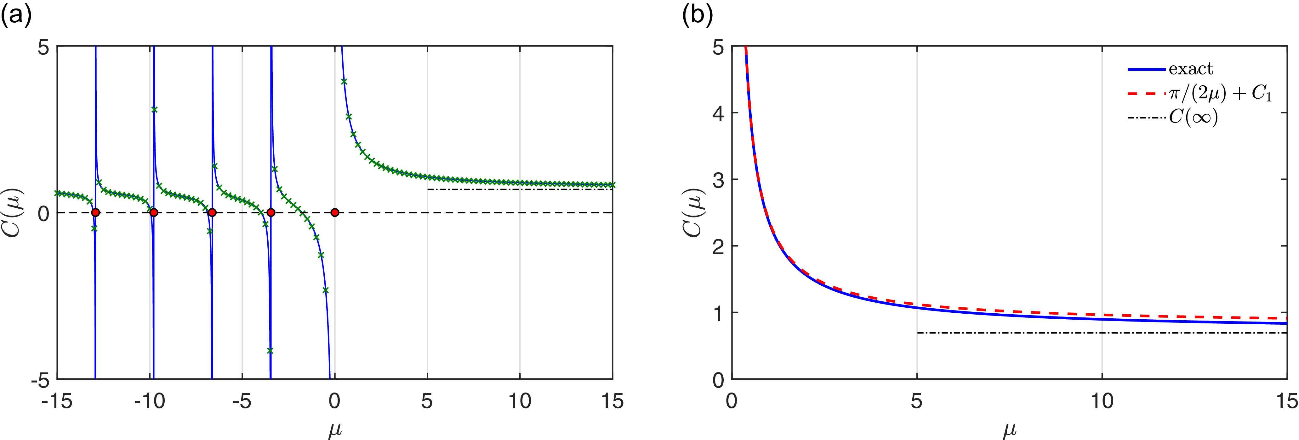


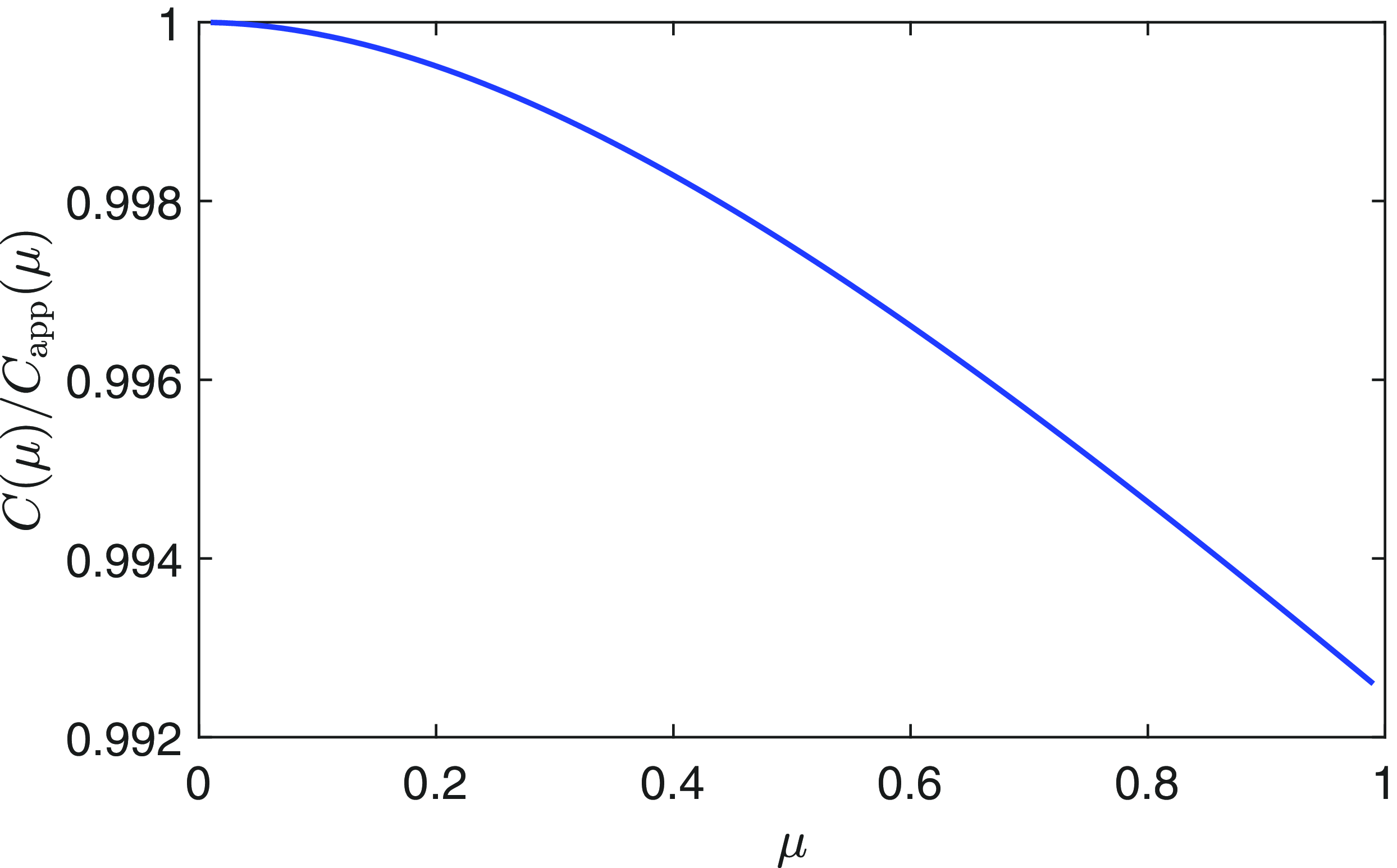


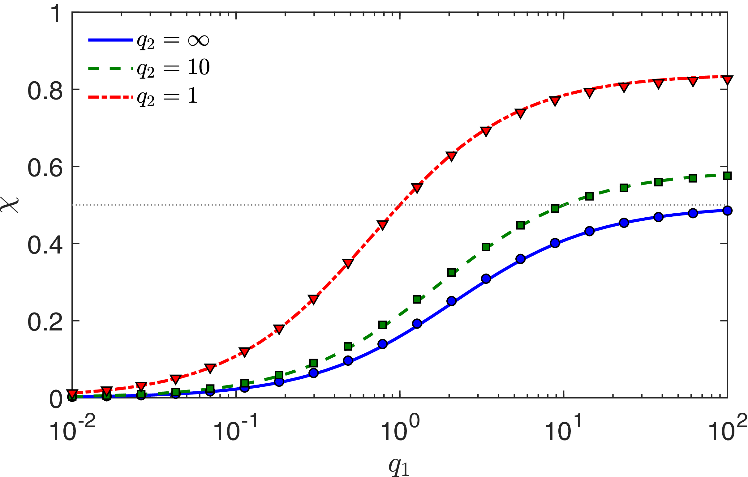


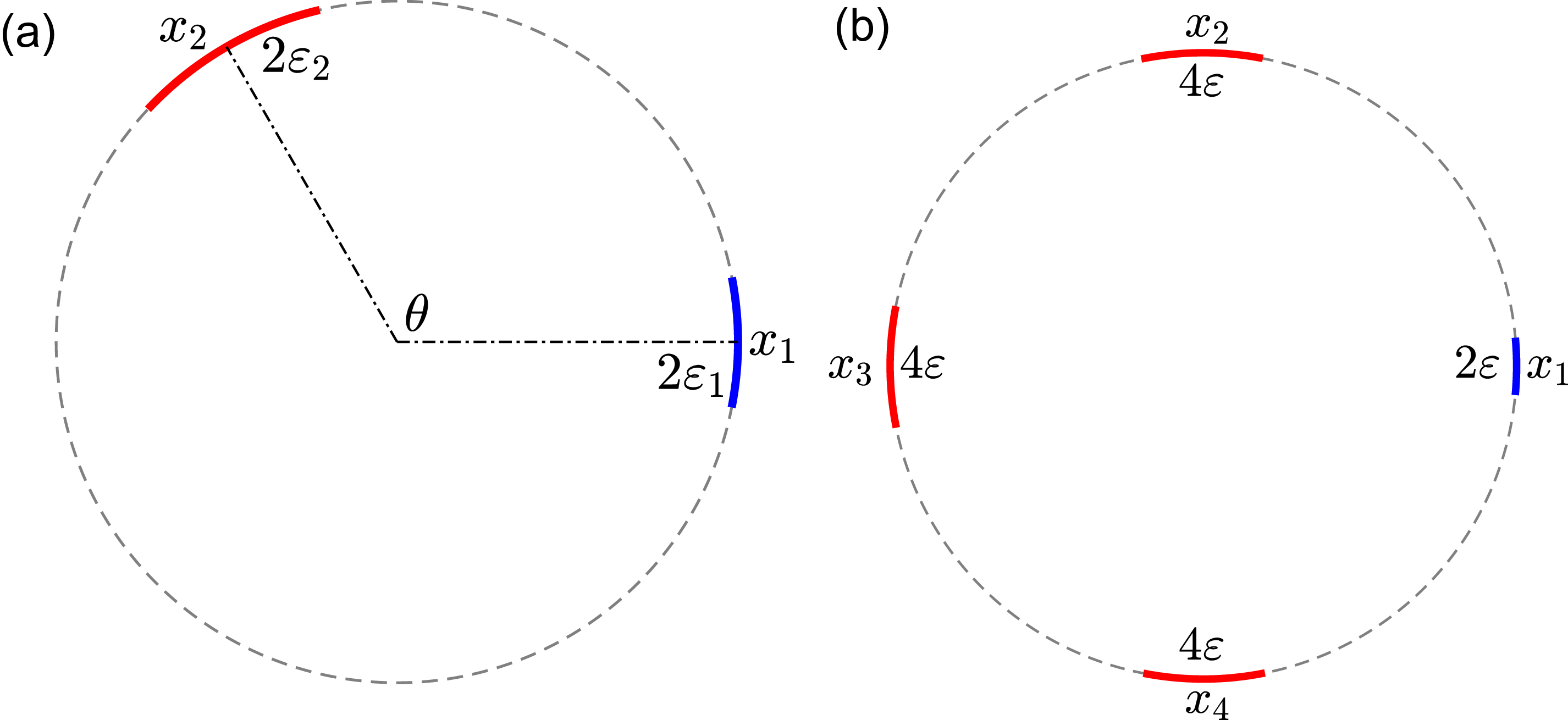


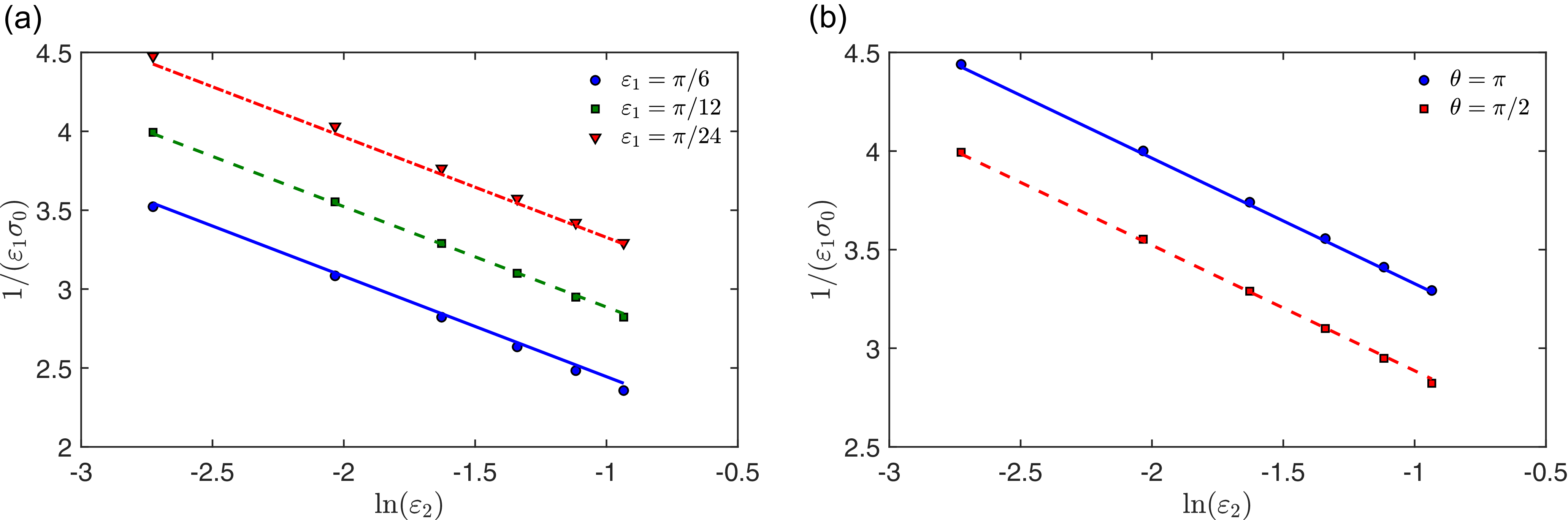


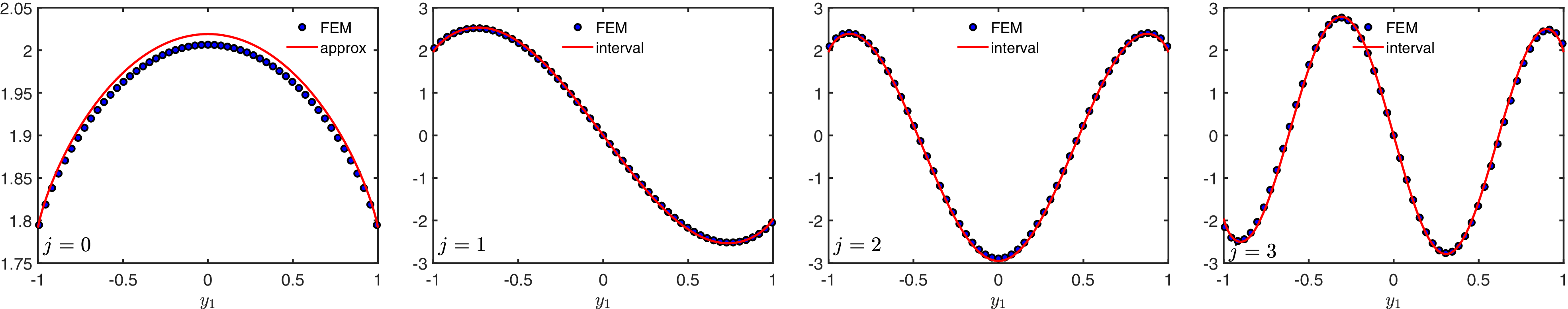


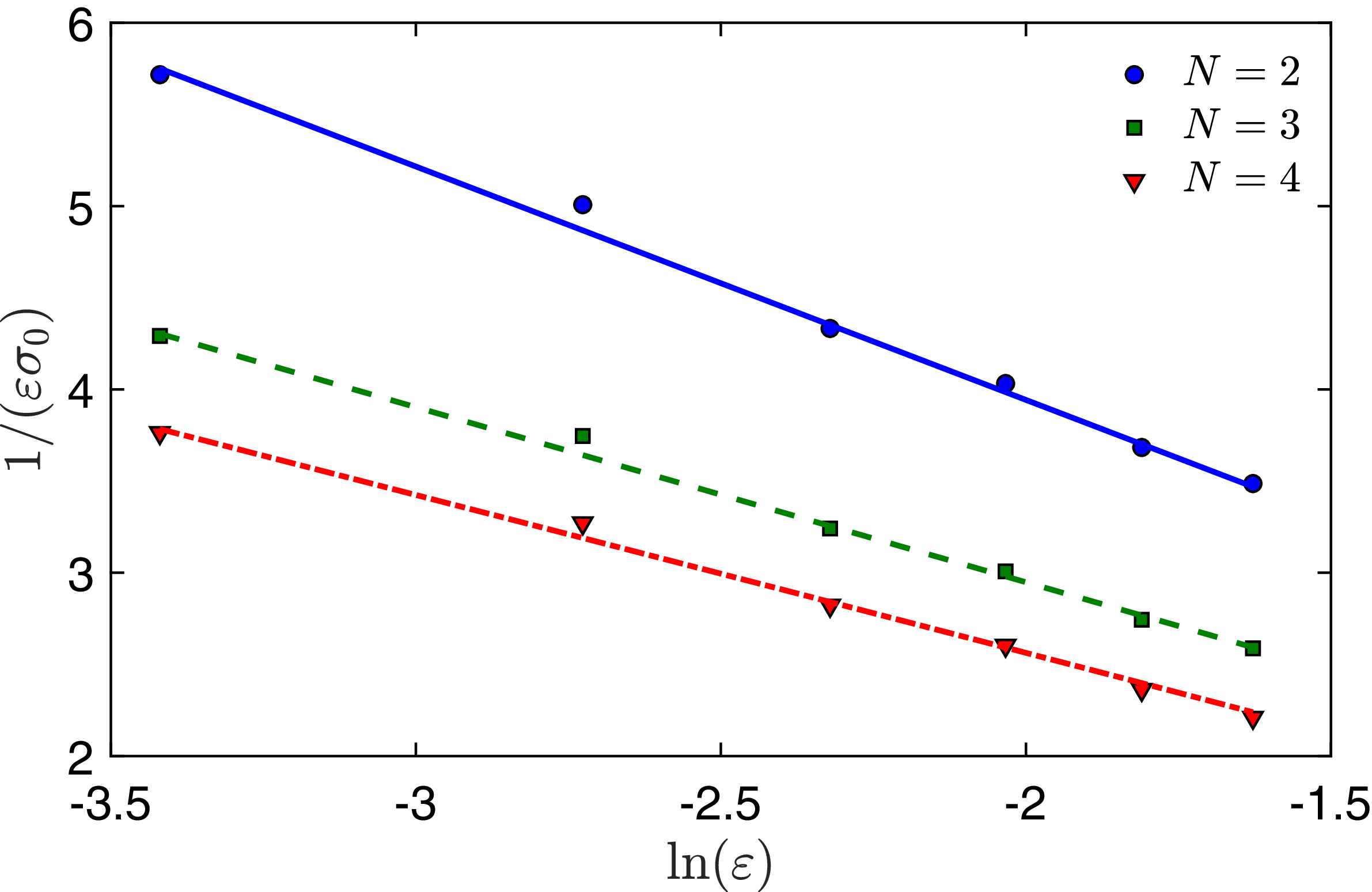


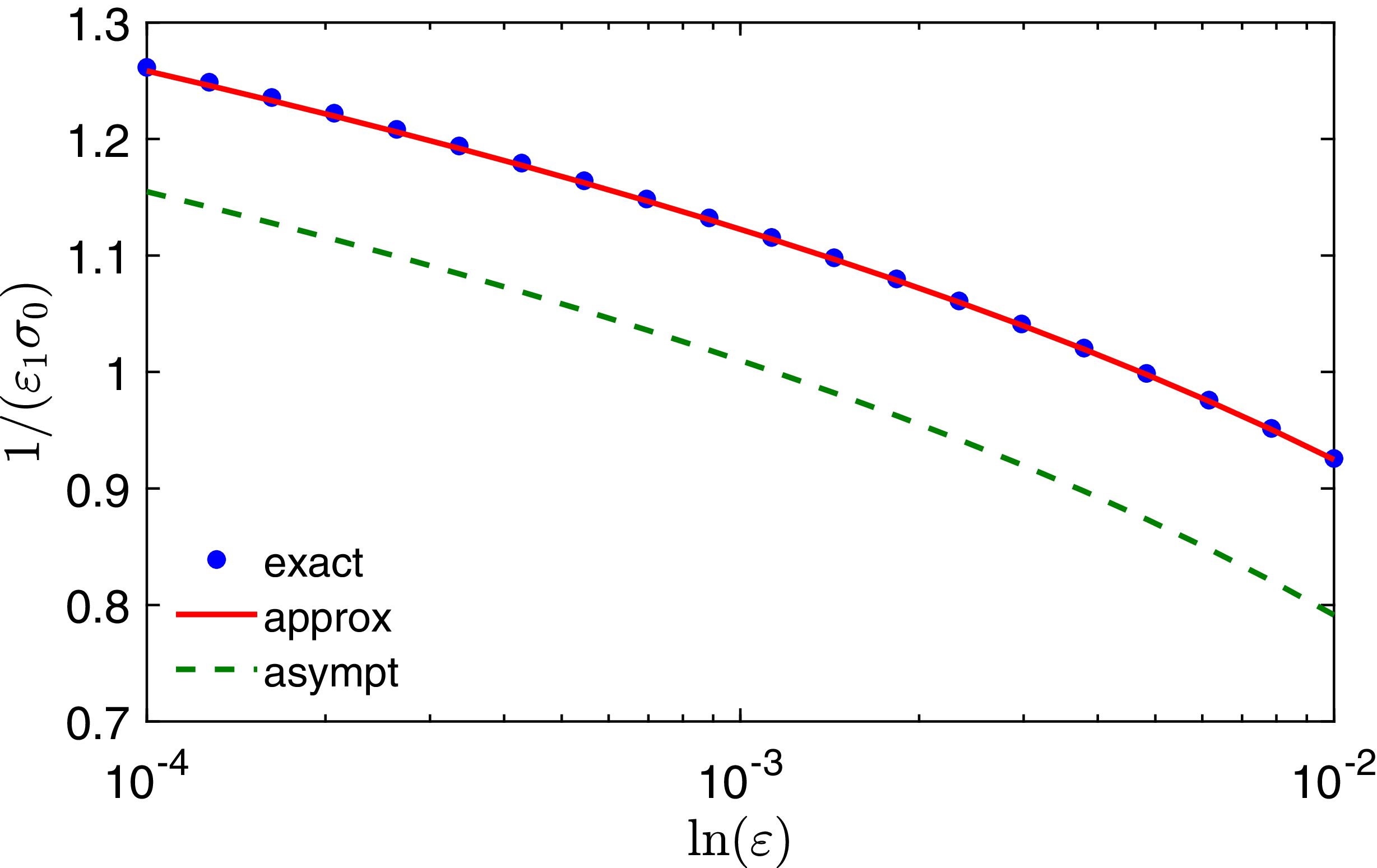


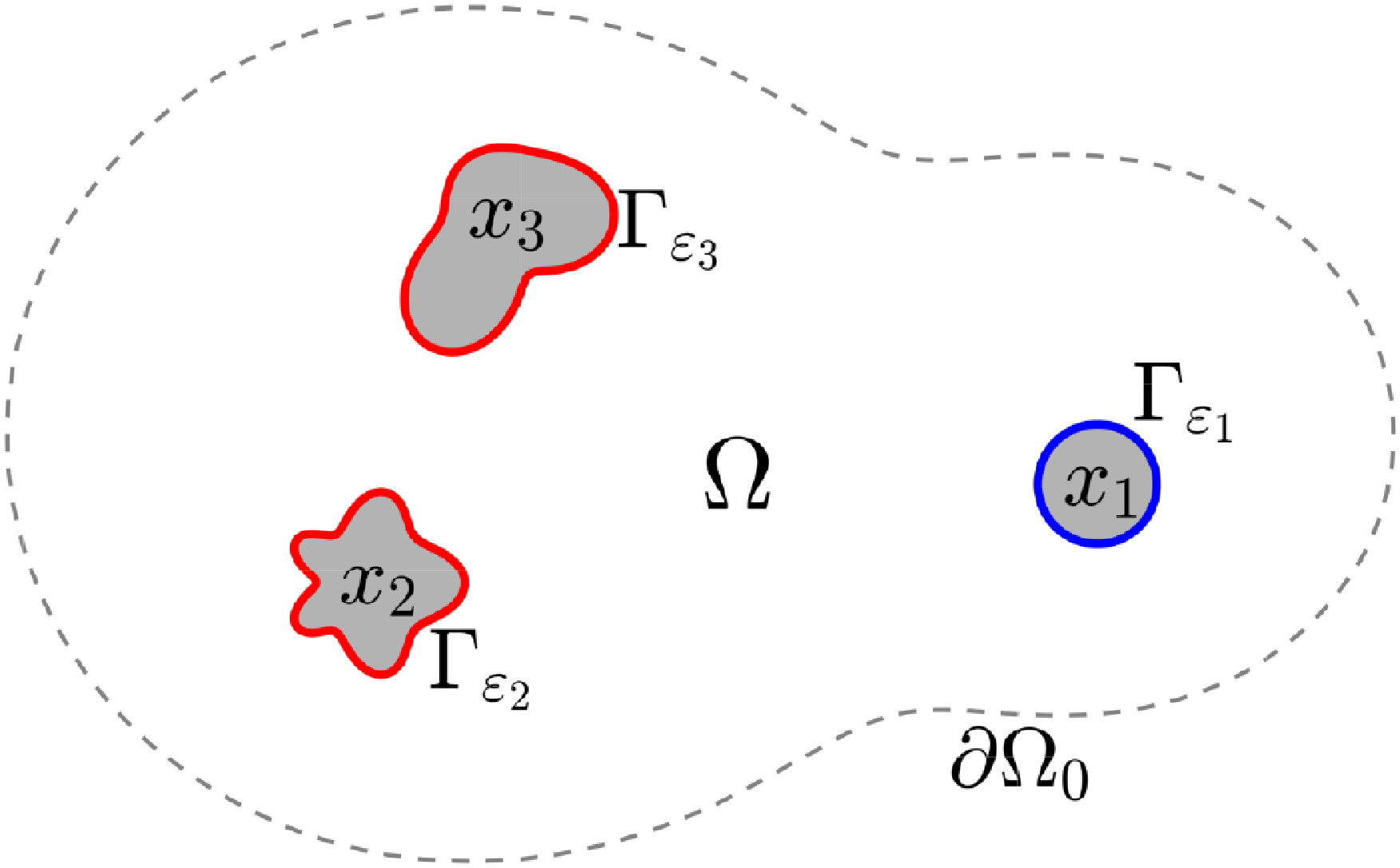


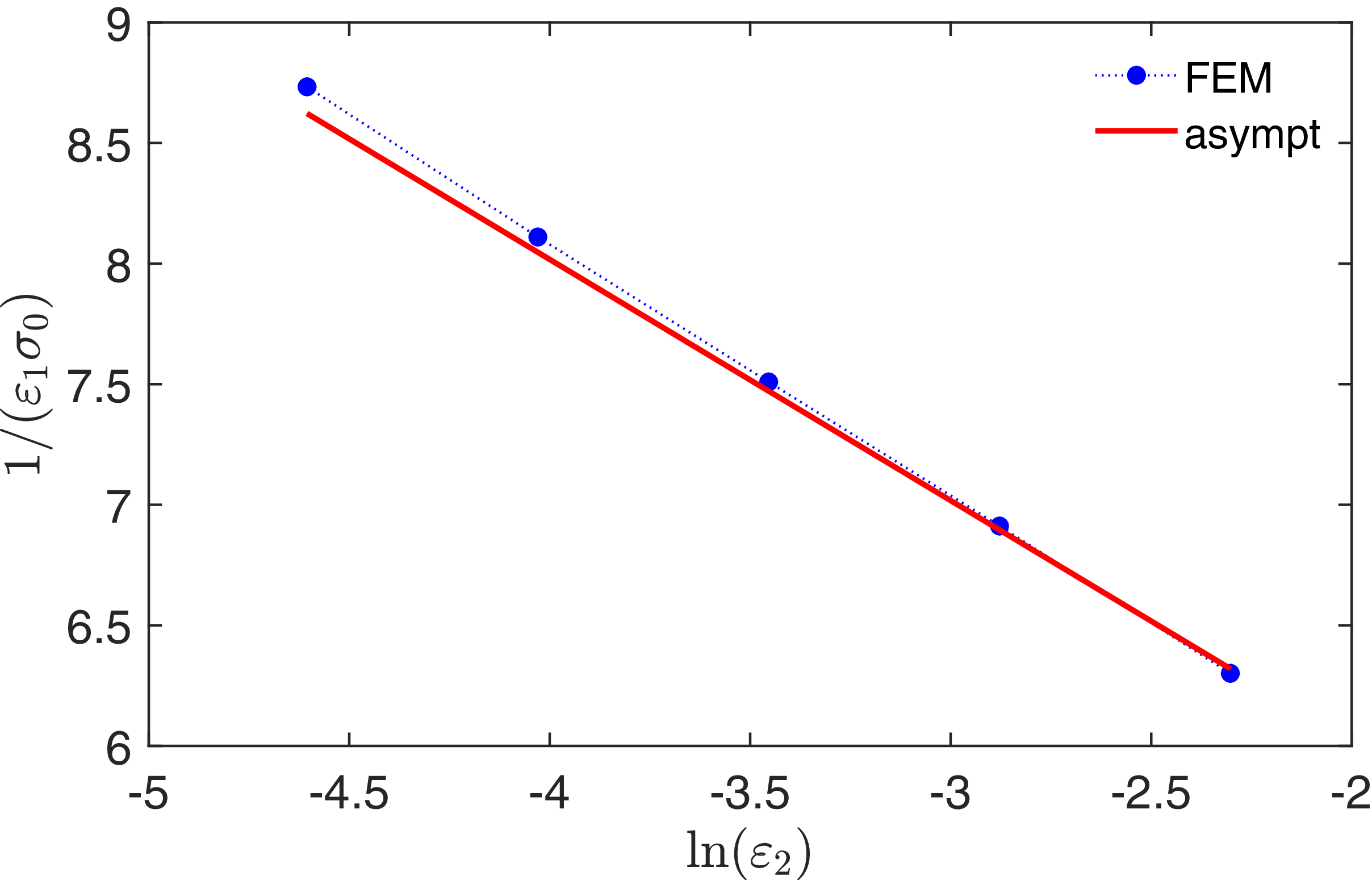


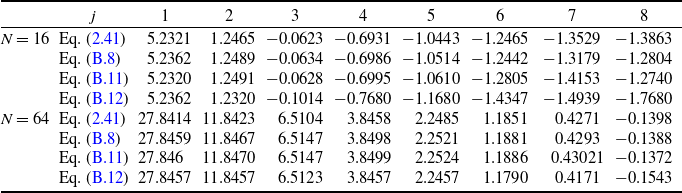

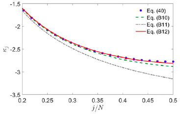


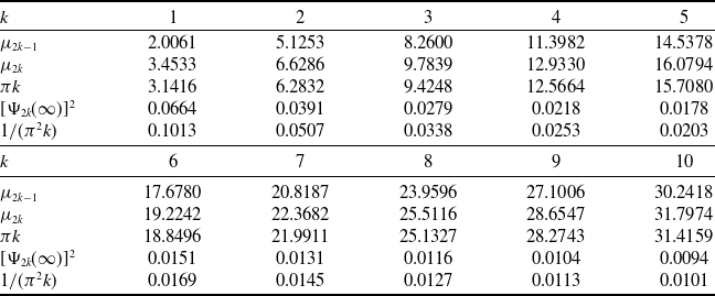


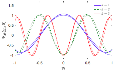


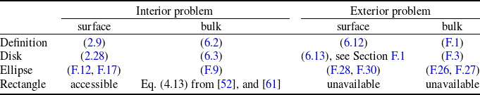

 Open access