1.1 Introduction
This chapter provides an introduction to the main features of the atmospheric general circulation and climate dynamics of the Southern Hemisphere (SH) troposphere, including the role of weather systems. The goal is to explain, in broad terms, the physical mechanisms shaping SH tropospheric climate for a reader without a background in atmospheric general circulation and climate dynamics. The stratosphere and the ocean circulation are only discussed tangentially.
Although this chapter concerns the SH, most of our figures show both hemispheres, and we refer to the Northern Hemisphere (NH) from time to time. This is partly because many climate phenomena are common to both hemispheres and partly in order to highlight the distinctive features of the SH.
The general circulation of the SH troposphere is often treated from the perspective of the governing equations of the atmosphere, as expressed in terms of budgets and fluxes (e.g. Karoly et al., Reference Karoly, Vincent, Schrage, Karoly and Vincent1998). However, such a perspective invariably leads to an emphasis on the zonal mean. Here we take a complementary and more phenomenological perspective starting from regional climatic features. This aligns with the current interest in understanding regional aspects of climate change and provides a foundation for other chapters in the monograph. We begin by describing these regional climatic features through spatial maps of key dynamical fields based on reanalysis. We then explain those features in terms of phenomena anchored in dynamical theory, such as monsoon circulations and storm tracks, including their zonal asymmetries. Our discussion covers tropical, subtropical, midlatitude, and high-latitude tropospheric phenomena, and the connections between them. The chapter concludes with a brief discussion of how the regional phenomena discussed here are expected to respond to climate change.
To begin the discussion, define some key terminology, and set the stage for the rest of the chapter, we start with the distribution of land masses and the Köppen–Geiger climate zones shown in Figure 1.1a. What is immediately apparent from the map is that the SH is primarily ocean, with most of the world’s land masses situated in the NH. On the other hand, the high-latitude SH consists of a continental land mass, Antarctica, surrounded by an ocean. (Note that for succinctness, we subsequently use the term ‘continental’ to refer to the major SH land masses outside of Antarctica.) These geographical features fundamentally shape the SH climate and its differences from the NH climate. The Köppen–Geiger climate zones were originally defined in the late nineteenth century from the consideration of biomes, but since biomes reflect local temperature and precipitation regimes (as indicated in the legend of Figure 1.1), these climate zones provide a good representation of the regional climatology.
(a) The Köppen–Geiger climate classification map (colours) and contours for sea surface temperature (SST in °C, ocean) and topography (land). Pann is the accumulated annual precipitation and Pth is a dryness threshold based on the absolute measure of the annual mean temperature and the annual cycle of precipitation (Kottek et al., Reference Kottek, Grieser, Beck, Rudolf and Rubel2006). (b,c) Precipitation (shading) and winds at 950 hPa (arrows) averaged over the periods (b) December–February (DJF) and (c) June–August (JJA). These are the SH summer and winter seasons, respectively; unless otherwise indicated, we use the terms ‘summer’ and ‘winter’ in this chapter to refer to SH summer and winter. The meteorological data here and in subsequent figures are based on the ERA5 reanalysis (Hersbach et al., Reference Hersbach2020) from 1979 to 2018.
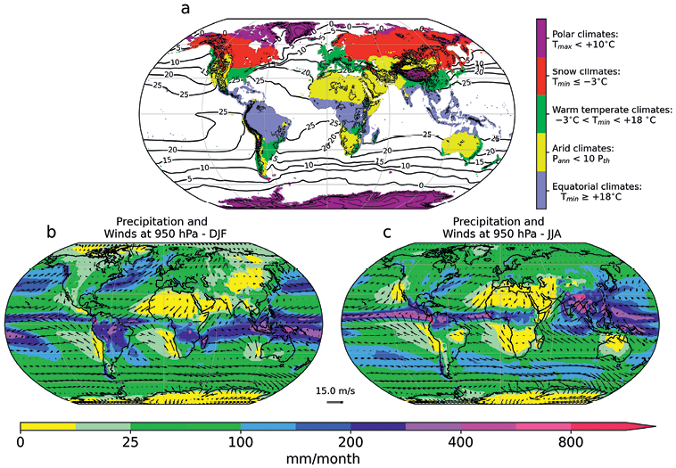
Figure 1.1 Long description
A three-panel figure displaying global maps on a Robinson pseudocylindrical projection, each showing different variables. The top panel presents the Köppen-Geiger climate classification in colour and topography in black contours over land, while black contours over the oceans represent sea surface temperature, ranging from 0 Celsius at high latitudes to 25 Celsius in the tropics. The colours highlight five climate types, namely polar, snow, warm temperate, arid, and equatorial. The bottom two maps display precipitation in colour and 950 hectopascal winds as arrows. The left panel represents the December to February mean, and the right panel represents the June to August mean, both based on ERA5 reanalysis from 1979 to 2018. Wetter areas, shaded in purple, are noticeably concentrated along the equatorial band, while dry areas, shown in yellow, are mainly over Antarctica and parts of Africa.
The equatorial climate zones are defined by the lack of a cold season; their extent is therefore largely determined by latitude, lying in the tropical regions within 23.5° of the equator where the Sun passes overhead twice a year. A band of heavy precipitation extends around the globe within the tropics, migrating farther poleward over continents in the summer hemisphere. Over the oceanic regions, the equatorial belt of deep convection is known as the Intertropical Convergence Zone (ITCZ) and is manifest in the precipitation and converging low-level trade winds shown in Figure 1.1b,c. Over land, the three continental sectors in the SH exhibit a pronounced seasonal cycle of precipitation, with heavy precipitation extending throughout the equatorial zone during summer, driven by the regional monsoon circulations that result from the seasonal cycle of insolation (Figure 1.1b). During winter, the monsoon rains move into the NH and the SH monsoon regions transition into their dry phase (Figure 1.1c). Thus, the continental equatorial climate zones experience heavy precipitation during some parts of the year, with the seasons corresponding to wet and dry. The equatorial small islands distant from continental regions may or may not do so, depending on their location.
In contrast to the equatorial climate zones, the polar climate zones are defined by the lack of a warm season. In the SH, polar climates are mainly found across Antarctica, as well as at the southernmost tip of South America (which lacks a warm season because it protrudes into the cold Southern Ocean). There are no snow climates to be found in the SH because of the absence of extensive subpolar land masses. The fact that the polar climate zones cover the entirety of the SH high latitudes has profound implications for climate and climate change across the SH.
Between the equatorial and polar climate zones, the picture is more complex with both arid and warm temperate climates existing at the same latitudes. Evidently, the climate zones in these subtropical and midlatitude regions are determined by precipitation, which is shaped by the atmospheric circulation together with the effects of topography. During summer in the SH subtropics, heavy precipitation is concentrated over the Subtropical Convergence Zones (STCZs), which extend from the east of the American, African, and Maritime continents into the Atlantic, Indian, and Pacific Oceans, respectively (Figure 1.1b), and are responsible for the warm temperate subtropical climates. In the midlatitudes, consistent with the climatological westerlies (Figure 1.1b,c), extratropical cyclones move along storm tracks into the west coasts of the continents, which leads to wet conditions there, particularly in winter. Elsewhere – either in the subtropics outside of the convergence zones, or in the midlatitudes where topography leads to rain-shadow regions – the arid climates are found. These various features of the atmospheric circulation unfold differently in the different continental sectors of the SH, leading to their distinct regional climates (Figure 1.1a).
The rest of the chapter is structured as follows. Section 1.2 reviews the basic zonal-mean features of the SH general circulation, to provide overall context, and then presents a series of spatial maps of key dynamical features, expanding on Figure 1.1b,c. Sections 1.3–1.6 then explain those features in terms of phenomena anchored in dynamical theory for the tropics, the subtropics, the midlatitudes, and the high latitudes, respectively. We briefly touch on the implications for regional climate change in Section 1.7.
1.2 Description of the General Circulation
1.2.1 Zonal Mean
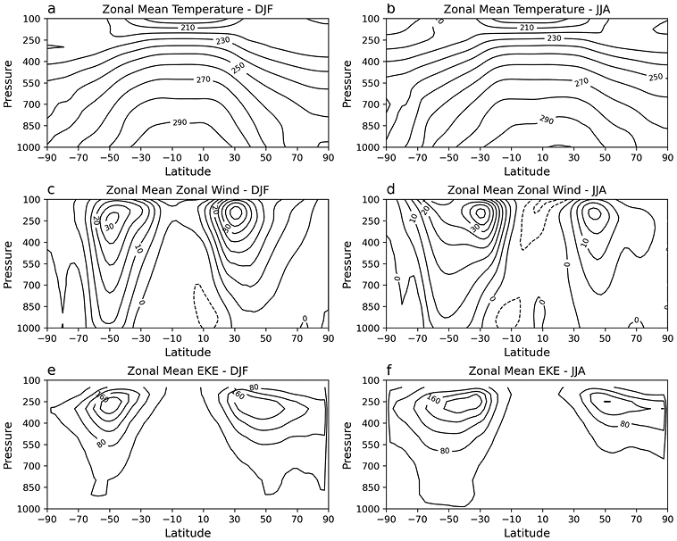
Figure 1.2 depicts the most salient features of the zonal-mean circulation. Figure 1.2a,b shows the zonal-mean cross-section of temperature for the two solstice seasons. Within the tropics, the meridional gradient is close to zero, not only because temperature peaks in the tropics but also because balanced flow for a small Coriolis parameter is possible only for weak horizontal temperature gradients (Held and Hoskins, Reference Held, Hoskins and Saltzman1985). Compared to the NH, there is little difference in the midlatitude temperature gradients between winter and summer in the SH, because the SH high latitudes remain cold year-round. Figure 1.2c,d shows the zonal-mean zonal wind, which is in thermal-wind balance with the temperature. In the tropics, weak surface easterlies (the trade winds) are evident in the winter hemisphere. Elsewhere the zonal-mean winds are generally westerly. In midlatitudes, the strength of the meridional temperature gradient is reflected in the strength of the zonal winds, with an upper tropospheric wind maximum (since the meridional temperature gradients change sign in the lower stratosphere). In the SH, the surface winds reach their maximum around 50°S (the surface westerlies) in both seasons. Whilst the SH zonal wind structure is vertically aligned in summer, there is a more complex vertical structure in winter which reflects the existence of a double-jet structure over the Pacific (see Figure 1.8d and further discussion in Section 1.5). The midlatitude jets are associated with storm tracks, whose synoptic time-scale transient eddy kinetic energy (EKE) (Figure 1.2e,f) also reaches its maximum in the upper troposphere together with the zonal jets.
Latitude-pressure cross-section of zonal-mean (a,b) temperature, (c,d) zonal wind, and (e,f) transient eddy kinetic energy (EKE), averaged over DJF and JJA, respectively. A 10-day high-pass Lanczos filter was applied to the daily wind values before computing EKE in order to capture the synoptic time-scale transient component. Contour intervals are 10 K, 5 ms−1, and 40 m2s−2. Dashed lines indicate negative values.
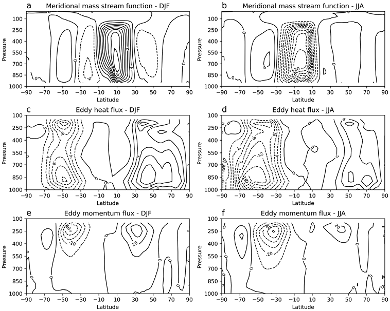
The troposphere acts as a classical ‘heat engine’ (Lorenz, Reference Lorenz1967), redistributing moist static energy (the appropriate generalisation of heat for the atmosphere) from warmer low latitudes to cooler high latitudes. Figure 1.3a,b shows the meridional mass stream function. The most notable feature is a strong cross-equatorial cell during the solstice seasons, with rising air on the summer side of the equator and sinking air extending to about 30° latitude on the winter side. Because the geopotential flux at upper levels dominates over the opposing heat and moisture fluxes at lower levels, the net effect is to transport moist static energy from the summer hemisphere deep into the winter hemisphere. This structure is known as the Hadley cell and reflects the summertime enhancement of tropical convection from the ITCZ and monsoons discussed in Section 1.1. As will be discussed later, however, the Hadley cell is not a single circulation and needs to be considered as an aggregation over regionally distinct phenomena. In the midlatitudes, the poleward moist static energy transport is accomplished not by the mean meridional circulation but instead by eddies (departures from the zonal mean), primarily by the meridional eddy heat flux which peaks near the surface (Figure 1.3c,d). In the SH, the eddy heat flux is primarily accomplished by transient eddies associated with baroclinic instability and storm tracks. This is in contrast to the NH where the stationary waves also play a significant role.
Latitude-pressure cross-section of the (a,b) meridional mass stream function, and zonal-mean (c,d) eddy heat flux [ ] and (e,f) eddy momentum flux [
 ], averaged over DJF and JJA, respectively. Contour intervals are 2 × 10¹⁰ kg s−1, 2 Kms−1, and 10 m2s−2.

The transient eddies also transport momentum poleward, and their momentum flux peaks, like their EKE, in the upper troposphere (Figure 1.3e,f). Consideration of the momentum budget lends further insight into the zonal-mean general circulation. In the vertical column, there is a balance between momentum flux convergence in the free atmosphere and surface friction. Hence in midlatitudes where the surface winds are strong and need to be maintained against surface friction, the jet is often considered to be eddy-driven. This phenomenon is also associated with baroclinic instability (Held and Hoskins, Reference Held, Hoskins and Saltzman1985). In the SH, this vertical alignment between upper-level momentum flux convergence and surface winds, mediated by the mean meridional mass circulation, is a clear feature around 50°S in both solstice seasons (Figure 1.3a,b,e,f). In the subtropics of the winter hemisphere, the situation is different, as with weak surface winds the dominant balance is instead between the poleward transport of (angular) momentum in the upper branch of the Hadley cell and the export of momentum from this region by the eddies. In fact, one can regard the transient eddy momentum fluxes as acting as a brake on the winter-hemisphere extent of the solstitial Hadley cell and thereby controlling the location of the subtropical descent zones (Schneider, Reference Schneider2006). In summary, the zonal-mean energy and momentum budgets are tightly linked through both the eddies and the mean meridional circulation.
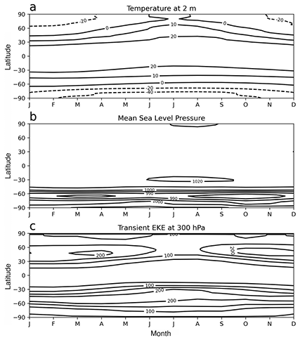
The full seasonal cycle is shown for a few key zonal-mean fields in Figure 1.4. For surface temperature (Figure 1.4a), outside high latitudes, the seasonal cycle is much weaker in the SH compared to the NH. On the other hand, for mean sea-level pressure (Figure 1.4b), the NH shows hardly any seasonal variation (in the zonal mean), whilst the SH exhibits a pronounced Semi-Annual Oscillation (SAO) in the mid-to-high latitudes, with minima during the equinox seasons. This curious feature is discussed in Section 1.5. Finally, the upper tropospheric transient EKE, indicative of storm track activity, exhibits a pronounced seasonal cycle in the NH, but in the SH, there is strong EKE throughout the year, which migrates poleward in both equinox seasons in conjunction with the SAO (Figure 1.4c).
Month-latitude cross-section of (a) 2 m temperature, (b) mean sea-level pressure, and (c) transient eddy kinetic energy (EKE) at 300 hPa. Note that the contour intervals are uneven in (a), with intervals of 10°C for positive values and 20°C for negative values. Contour intervals are 10 hPa and 50 m2s−2 for (b) and (c), respectively.

1.2.2 Longitudinal Structure
We now turn to the spatial maps that (together with Figure 1.1) provide the main foundation for the rest of the chapter. As with Figure 1.1, the chosen fields are first presented as global maps for the two solstice seasons. A few selected fields are also presented as polar stereographic maps for all four seasons, in order to better represent the SH high latitudes and to show the full seasonal evolution. The two presentation formats thereby provide complementary perspectives for those fields. Unless indicated otherwise, the shading is only provided for visual clarity. The discussion here is quite brief and largely descriptive, with more explanatory perspectives provided in Sections 1.3 to 1.6.
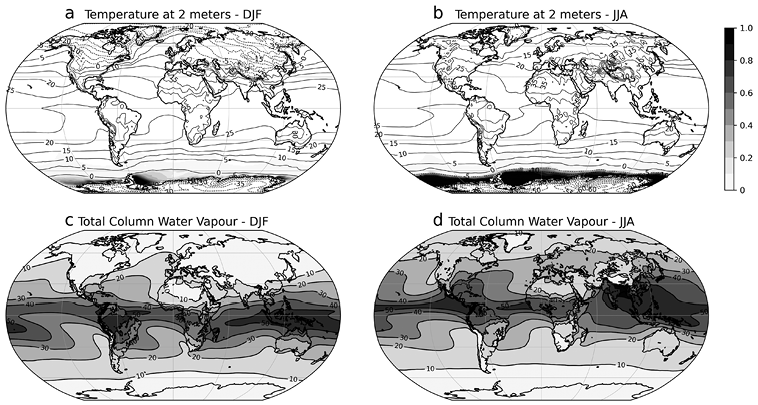
Near-surface (2 m) temperature (Figures 1.5a,b and 1.6a,d,g,j) largely reflects the features seen in the zonal mean (Figure 1.4a), with notable zonal asymmetries associated with the cold sea surface temperatures (SSTs) due to upwelling along the west coasts of South America and Africa, and around Antarctica where the zonal asymmetries are also apparent in the sea-ice fraction. The seasonal cycle of temperature is larger over land than over ocean, but this contrast in seasonality between land and ocean regions is much weaker in the SH than it is in the NH, due to the much smaller continental land masses in the SH. Antarctica is the exception, together with the surrounding ocean regions where the sea-ice extent is highly seasonal. Over the oceans, the regions with higher surface temperature are regions of comparatively high evaporation which then coincide with the regions of higher total column water vapour (shaded regions in Figure 1.5c,d). Over land, the regions with higher total column water vapour are instead associated with moisture transport driven by the monsoon circulations. Total column water vapour tends to be high where precipitation is high, not only in the monsoons but also in the ITCZ and the summertime STCZs. The convergent low-level winds in these regions are transporting moisture upgradient to fuel the large-scale convection (Figure 1.1b,c).
(a,b) 2 m temperature and sea-ice fraction (shading) and (c,d) total column water vapour, averaged over DJF and JJA, respectively. Contour intervals are 5°C and 10 kg m−2.

Figure 1.5 Long description
A four-panel figure showing global maps on a Robinson pseudocylindrical projection. The top left panel shows contours of December to February mean temperature at 2 metres ranging from -60 Celsius at high latitudes to 25 Celsius in the tropics, with greyscale shading representing sea-ice fraction, concentrated around Antarctica. The top right panel represents the same variables for the June to August mean. The bottom panels illustrate total column water in greyscale shading, with values ranging from 10 kilograms per metre squared at high latitudes and 50 kilograms per metre squared in the equatorial region. The left panel shows the December to February mean, and the right panel shows the June to August mean.
(a,d,g,j) 2 m temperature (contours) and sea-ice fraction (shading), (b,e,h,k) mean sea-level pressure, and (c,f,i,l) precipitation, averaged over DJF, March–May (MAM), JJA, and September–November (SON), respectively. Contour intervals are 5°C and 10 hPa for the first two sets of panels. Note the unequal contour intervals for precipitation, which are marked in units of mm month–1.
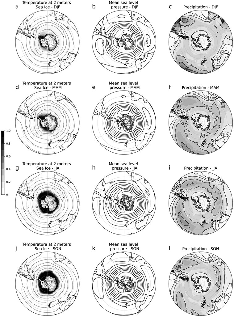
Figure 1.6 Long description
The figure presents 12 maps of Southern Hemisphere climatologies in a polar projection with Antarctica at the centre and land masses south of 20 south at the edges. Each row shows a season, ordered from top to bottom, namely December to February, March to May, June to August, and September to November. Each column displays a different variable. The left column shows 2-metre temperature in black contours at 5 Celsius intervals, with sea-ice fraction shaded in greyscale. The middle column depicts mean sea-level pressure in 10 hectopascal intervals. The right column shows precipitation in millimetres per month.
The large-scale convection in the tropics is reflected not only in precipitation but also in outgoing longwave radiation (OLR) (Figure 1.7a,b) and in the divergence of upper-tropospheric horizontal wind (Figure 1.7c,d). The OLR is small where the cloud tops are highest (and thus coldest), indicating the most vigorous convection, whilst the upper-tropospheric divergence is positive where the upward motion is strongest. These features are seen to be co-located with the regions of most intense precipitation (Figure 1.1b,c). In contrast, OLR is large (shaded regions in Figure 1.7a,b) where skies are clear, indicative of large-scale descent and a lack of precipitation. Such regions occur in the subtropics to the west of the continental sectors and are associated with the Subtropical Anticyclones (Figures 1.8a,b and 1.6b,e,h,k; see also Figures 1.1b,c and 1.6c,f,i,l), which are themselves responsible for the coastal upwelling and low SSTs in those regions.
(a,b) Outgoing longwave radiation and (c,d) divergence of horizontal wind at 200 hPa, averaged over DJF and JJA, respectively. Contour intervals are 20 Wm−2 and 1 s−1. Dashed lines indicate negative values.
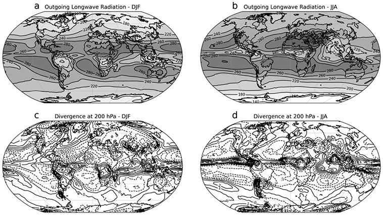
Figure 1.7 Long description
The figure shows four maps on a Robinson pseudocylindrical projection with December to February mean values in the left column and June to August mean in the right column. The top maps show outgoing longwave radiation in greyscale shading, with darker colours representing larger values and black contour intervals of 20 Watts per square metre superimposed. The bottom maps show 200 hectopascal horizontal wind divergence in contours, with positive values in solid black lines and negative values in dashed lines, varying at 1 per second intervals.
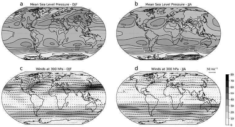
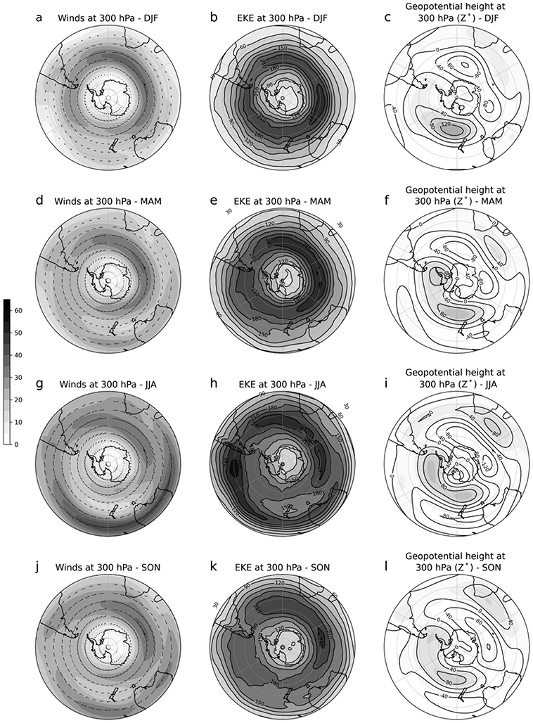
We finally turn to a few fields that are particularly relevant for explaining regional climate in the extratropics. Figures 1.8c,d and 1.10a,d,g,j show the upper-level winds, and Figures 1.9a,b and 1.10b,e,h,k show the upper-level transient EKE, which is seen to be closely related to the extratropical winds. During summer, the zonal variations in the extratropics are mainly in the strength of the features, with the jet speed somewhat stronger over the southern Atlantic and Indian Oceans, compared to over the Pacific. During winter and spring, however, the jet (and EKE) exhibits large zonal asymmetries. In particular, it has a single (albeit broad) structure over the Atlantic and the western Indian Ocean, and splits over the eastern Indian Ocean, spiralling towards Antarctica in the south and intensifying over Australia in the north. Over the Pacific, it exhibits a double-jet structure.
(a,b) Mean sea-level pressure and (c,d) horizontal wind speed (shading) and vectors (arrows) at 300 hPa, for DJF and JJA, respectively. Contour intervals are 10 hPa and 10 ms−1.

Figure 1.8 Long description
This figure shows four maps on a Robinson pseudocylindrical projection, with December to February mean values in the left column and June to August mean values in the right column. The top maps display mean sea level pressure in greyscale shading with darker colours representing larger values and black contour intervals of 10 hectopascals superimposed. The bottom maps show 300 hectopascal horizontal wind speed in greyscale shading at intervals of 10 metres per second, with vectors superimposed.
(a,b) Transient eddy kinetic energy (EKE) at 300 hPa and (c,d) deviation from the zonal mean of geopotential height at 300 hPa, for DJF and JJA, respectively. A 10-day high-pass Lanczos filter was applied to the daily wind values before computing EKE in order to capture the synoptic time-scale transient component. Contour intervals are 30 m2s−2 and 40 m.
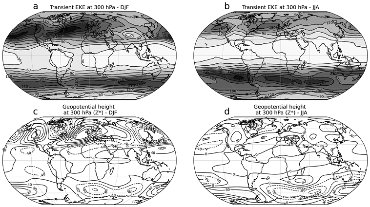
Figure 1.9 Long description
This figure shows four maps on a Robinson pseudocylindrical projection, with December to February mean values in the left column and June to August mean values in the right column. The top maps show 300 hectopascal transient eddy kinetic energy in greyscale shading with darker colours representing larger values and black contour intervals of 30 metres squared per second squared superimposed. The bottom maps show 300 hectopascal deviation from zonal mean geopotential height in contours, with positive values in solid black lines and negative values in dashed lines, varying at 40 metre intervals.
(a,d,g,j) Horizontal wind speed (shading) and vectors (arrows) at 300 hPa, (b,e,h,k) transient EKE at 300 hPa, and (c,f,i,l) deviation from the zonal mean of geopotential height at 300 hPa, averaged over DJF, MAM, JJA, and SON, respectively. Contour intervals are 5 ms−1, 30 m2s−2, and 40 m.

Figure 1.10 Long description
The figure presents 12 maps of Southern Hemisphere climatologies, south of 20 south, in a polar projection with Antarctica at the centre. Each row shows a season, ordered from top to bottom, namely December to February, March to May, June to August, and September to November. Each column displays a different variable. The left column shows 300 hectopascal horizontal wind speed in greyscale shading at intervals of 5 metres per second, with vectors superimposed. The middle column shows 300 hectopascal transient eddy kinetic energy in greyscale shading with darker colours representing larger values and black contour intervals of 30 metres squared per second squared superimposed. The right column shows 300 hectopascal deviation from zonal mean geopotential height in contours, varying at 40 metre intervals, with the strongest positive values shaded.
The zonal asymmetries in the extratropical circulation are generally explicable in terms of stationary Rossby waves, which can be forced by topography or surface thermal contrasts (including SST patterns). To help identify the stationary waves, Figures 1.9c,d and 1.10c,f,i,l show the deviation from the zonal mean of the upper-level geopotential height.
1.3 Climate Dynamics of the Tropics
The near-equatorial regions of the Earth, referred to as the tropics, are generally warm and moist in comparison to other regions. While there is no hard boundary separating tropics from extratropics from a meteorological perspective, there are key characteristics differentiating the two regions. For example, the seasonal variation of temperature in the tropics is relatively small, within a few degrees, compared to the extratropics (Figure 1.4a). Therefore, in contrast to four astronomical seasons, defined by solar insolation and hence temperatures, the tropics have alternating wet and dry seasons. The timing of the wet and dry seasons in any particular location depends on the seasonal movement of the tropical convergence zones shown in Figure 1.1b,c and is not necessarily aligned with the astronomical seasons.
Another key feature of the tropics is the organised convection, which is the main phenomenon driving tropical circulation systems. Although the Coriolis force is relatively weak in the tropics, it still plays an important role in the organisation of the tropical atmosphere at synoptic scales. Certain atmospheric waves owe their existence to the poleward gradient of planetary rotation in the tropics and are often associated with tropical diabatic heating due to deep convection (Matsuno, Reference Matsuno1966; Gill, Reference Gill1980).
The meteorology of the tropics is mainly characterised by the large-scale climatological features, including the trade winds, the ITCZ, and the monsoons, and synoptic-scale systems such as tropical cyclones (TC), low-level jets, tropical pressure and heat lows (e.g. Angola, Kalahari, and West Australia). Land-ocean-atmosphere interactions associated with topography, forests, and lakes also alter the local climatology. We now describe some of these key features.
1.3.1 Tropical Convection
Deep tropical convection acts as a driver for the global climate by distributing water, energy, and momentum within the earth system. For instance, latent heat release by convection provides a source of energy for the global atmospheric circulation (Riehl and Malkus, Reference Riehl and Malkus1958), whereas clouds associated with deep convection modify the Earth’s radiation budget (e.g. Bony et al., Reference Bony, Semie, Kramer, Soden, Tompkins and Emmanuel2020).
Deep tropical convection is associated with the upward branch of the Hadley cell and divergence in the upper troposphere (Figure 1.7c,d). This divergent flow then converges in the subtropics, affecting the subtropical anticyclones, westerly jets, and extratropical weather systems through planetary-wave activity (Hoskins and Karoly, Reference Hoskins and Karoly1981). Over the ocean, the most prominent feature that reflects tropical deep convection is the narrow band of heavy rainfall and low OLR (Figure 1.7a,b) that extends across the equatorial oceanic regions, also called the ITCZ. Over land, the majority of deep convection is located over the large continental landmasses and is manifest as regional monsoons.
Historically the ITCZ and regional monsoons have been seen as dynamically distinct phenomena, and there have been differing views over which regional climatic features qualify for which designation. More recently, the view has emerged that both phenomena represent different regional manifestations (and dynamical regimes) of a global monsoon arising from the seasonal migration of the tropical convergence zones (e.g. Geen et al., Reference Geen, Bordoni, Battisti and Hui2020). This explains why the distinction between ITCZ and regional monsoon can become fuzzy in particular regions. Moreover, in the SH the tropical convergence zones can merge with the STCZs, which are unique to the SH (Section 1.4.2).
1.3.2 The Intertropical Convergence Zone (ITCZ)
The ITCZ is characterised by the band of lowest pressure near the equator (Figure 1.8a,b) where the trade winds converge (Figure 1.1b,c), and there is high rainfall (Figure 1.1b,c). The ITCZ typically migrates seasonally following the Sun’s position with a lag of around 1–2 months, reaching its southernmost limit around January (~1 month lag from SH summer solstice) and its northernmost limit around July (~1 month lag from NH summer solstice). However, there are regional asymmetries and exceptions in the ITCZ migration (Figure 1.1b,c).
During JJA, the ITCZ is exclusively in the NH. However, in DJF, the ITCZ is located north of the equator over the Atlantic and Pacific Oceans and south of the equator over the Indian and western Pacific Oceans. Hence, in summer there is a double ITCZ over the west Pacific (Figure 1.1b). The hemispheric asymmetry in the ITCZ location has been explained by a number of mechanisms associated with moist atmospheric dynamics, including the meridional cross-equatorial energy flux and net energy input at the equator (e.g. Waliser and Somerville, Reference Waliser and Somerville1994; Bischoff and Schneider, Reference Bischoff and Schneider2016; Geen et al., Reference Geen, Bordoni, Battisti and Hui2020; Kang, Reference Kang2020).
1.3.3 Monsoons
During DJF, the seasonal migration of the tropical convergence zone manifests as regional monsoons over South America, southern Africa, and the Indo-Australian Maritime Continent region. The land-sea contrast and local orographic features play a key role in the poleward progression of the monsoon systems over different regions. The continental monsoons also extend further poleward than the oceanic ITCZ sectors owing to this contrast, except in the west Pacific, where the SH ITCZ merges with the South Pacific Convergence Zone (SPCZ) (see Section 1.4.2). These continental monsoons are visible in the climatological rainfall for SH summer (Figure 1.1b).
Monsoons are traditionally characterised by a seasonal reversal of prevailing surface winds, which primarily develop due to the difference in heating of the NH and SH during the solstice seasons, and associated precipitation. However, there are regional exceptions to this definition, such as Mexico and southwest United States and parts of South America and southern Africa, which do not exhibit a seasonal reversal in surface winds yet are generally recognised as monsoon regions (Webster, Reference Webster2020).
Variations in the regional monsoonal precipitation occur on a range of timescales from sub-daily to multi-decadal. The diurnal cycle is especially important in the near-coastal regions during the pre-monsoon and monsoon-break periods, resulting in significant amounts of afternoon precipitation during the summer months (Yang and Slingo, Reference Yang and Slingo2001). Much of the monsoon variability occurs on intra-seasonal timescales, with days to weeks of active rainfall interspersed with break periods of a similar length. The most dominant mode of intra-seasonal variability is the Madden–Julian Oscillation (MJO), which is an eastward-moving region of enhanced convection, tailed by a region of suppressed convection (Hendon and Liebmann, Reference Hendon and Liebmann1990, see also Section 5.3). However, other factors such as midlatitude troughs are also important for some regions, such as the Australian monsoon (Berry and Reeder, Reference Berry and Reeder2016). The year-to-year variations in the regional monsoons are largely driven by the oscillation in equatorial Pacific SSTs, referred to as El Niño Southern Oscillation (ENSO), through large-scale teleconnections. Other slowly varying land, atmospheric, and oceanic conditions, such as soil moisture (Koster et al., Reference Koster, Mahanama, Livneh, Lettenmaier and Reichle2010), snow cover (Sobolowski et al., Reference Sobolowski, Gong and Ting2010), the SSTs over the equatorial Indian Ocean (Saji et al., Reference Saji, Goswami, Vinayachandran and Yamagata1999), and stratosphere–troposphere interaction (Baldwin et al., Reference Baldwin, Stephenson, Thompson, Dunkerton, Charlton and O’Neill2003), also contribute to the interannual variability, although their influence is usually smaller in magnitude compared to ENSO. The interaction between the land, atmosphere, and ocean through internal processes, such as wind-evaporation feedback, also contributes to the interannual variability (e.g. Sekizawa et al., Reference Sekizawa, Nakamura and Kosaka2018). On multi-decadal timescales, the Interdecadal Pacific Oscillation (Power et al., Reference Power, Lengaigne, Capotondi, Khodri, Vialard, Jebri, Guilyardi, McGregor, Kug, Newman and McPhaden2021) is important, as are human-related activities such as changes in anthropogenic greenhouse gases (GHGs) and aerosol emissions (Wilcox et al., Reference Wilcox, Liu and Samset2020) or land-use and land-cover (Quesada et al., Reference Quesada, Devaraju, de Noblet‐Ducoudré and Arneth2017). Finally, changes in monsoonal rainfall and circulation are also impacted by multiple local factors, which we now describe.
1.3.4 Local Effects: Inland Water Bodies and Mountains
The presence of large inland water bodies, such as rivers and lakes, modulates the climate locally (see Section 5.2.3). They drastically change the surface energy and water balance in a given region, and hence its climate, through the mediation of flows of energy, moisture, and momentum. For instance, lakes alter the local circulation. During the day, a lake breeze leads to a cooling effect in the areas surrounding the lakes, whereas at night the flow reverses due to a land breeze. The total precipitation over a large inland water body is also generally higher than the surrounding areas, for example, Lake Victoria in Africa (Anyah et al., Reference Anyah, Semazzi and Xie2006; Thiery et al., Reference Thiery, Davin, Panitz, Demuzere, Lhermitte and Van Lipzig2015).
The interaction between large inland water bodies and mountains can lead to interesting phenomena. Mountainous areas can modify the thermal gradients at night between the land surface and the lake. The gradients are accentuated as the colder air from the mountain summit interacts with air down the valley and over land areas next to the lake. Thus, a stronger land breeze circulation is produced, leading to strong convection and precipitation over the lake (Anyah et al., Reference Anyah, Semazzi and Xie2006). Mountains on their own can also modify the climate over a region, by acting as a physical barrier and altering the large-scale circulation systems and precipitation. The Andes Mountains, for example, lead to orographically enhanced rainfall and wetter conditions over Colombia, which is on the windward side, and to drier conditions over Ecuador, which is in the mountain shadow region. Mountain ranges also affect the temperature over the region; temperatures are cooler over the Great Rift Valley in East Africa and also the Andes Mountains compared to the surrounding areas (Figure 1.5a,b).
In the SH, there are two major tropical rainforests, the Amazon rainforest in South America and the Congo rainforest in central Africa. The rainforest interacts with the atmosphere to provide moisture within the basins and thus influence the nearby climate. In particular, the Amazon region is the main source of moisture for central Brazil and the La Plata basin, and a similar role is played by the Congo rainforest in the precipitation regime of central and southern Africa.
1.3.5 Tropical Cyclones
Tropical cyclones (TCs) are among the most significant mesoscale phenomena in the tropics. They are characterised by warm-core, low-pressure systems, reaching up to a diameter of 1,000 km with cyclonically rotating winds and cloud bands. These differ in structure from extratropical storms as extratropical cyclones have a clear frontal system, which TCs do not have. TCs form over warm ocean water (>26°C) and primarily derive their energy from the release of latent heat through condensation. With the relatively cold SSTs over the tropical South Atlantic and the southeast Pacific, SH TCs mainly occur over the southwest and southern Indian Oceans, as well as the Maritime Continent warm pool and southwest Pacific, between November and April. After forming in the tropics, TCs drift westward, then curve to higher latitudes along an anticyclonic trajectory where the warm cores can transit into extratropical storms (Jones et al., Reference Jones, Harr, Abraham, Bosart, Bowyer, Evans, Hanley, Hanstrum, Hart, Laurette, Sinclair, Smith and Thorncroft2003). The locations of TC genesis, intensification, and maximum intensities in the SH are further poleward (17°–18°S) compared with the NH (~10°N) (Pillay and Fitchett, Reference Pillay and Fitchett2019). Further discussion of TCs can be found in Chapter 5.
1.4 Climate Dynamics of the Subtropics
The relatively dry latitudes between the wet tropics and the stormy midlatitudes are referred to as the subtropics. Most of the Earth’s major deserts are found at subtropical latitudes (approximately 20°–40°S and 20°–40°N). These dry regions are punctuated with very wet diagonally oriented convergence zones in the SH during the summer months (Figure 1.1b). The existence of subtropical dry zones may seem surprising at first glance, since the zonal average of important state variables such as temperature (Figure 1.2a,b) and humidity (Figure 1.5c,d) in the atmosphere decrease monotonically from the equator towards the poles. However, as will be discussed later, it is the motion of the atmosphere, which is externally driven by both the tropics and extratropics, that is most consequential for the subtropical climate.
1.4.1 The Subtropical High-Pressure Belt
The subtropical dry zones are co-located with a high-pressure belt sometimes referred to as the subtropical ridge. The subtropical ridge is present at all longitudes in the SH winter climatology and clearly defined into three semi-permanent anticyclones in the SH summer (Figure 1.8a,b). These near-surface attributes of the subtropical climate are symptomatic of the large-scale descent associated with meridional overturning of the Earth’s atmosphere, which in the zonal mean is called the Hadley cell, described earlier. But the subtropics are also associated with cooling by high-latitude transient eddies, as well as radiative cooling to space in the relatively clear and dry subtropical atmosphere (Trenberth and Stepaniak, Reference Trenberth and Stepaniak2003). In this sense the subtropics truly owe their defining characteristics to their function as a region connecting the tropics to the high-latitude regions of the Earth. Here we explore some of the key aspects of the subtropics and emphasise the importance of the asymmetries and transient features of the subtropical climate.
The mean latitudinal position of the subtropical ridge moves equatorward during winter and poleward during summer (Figure 1.8a,b), generally mirroring the seasonal meridional migration of the ITCZ. The SH subtropical high-pressure systems are considerably stronger in winter than in summer, particularly over the South Atlantic and southern Indian oceans, contrasting with the NH subtropical anticyclones, which are stronger in boreal summer than in boreal winter (Figure 1.8a,b). These differences are due to the different mechanisms that vary spatially and seasonally. Although the primary drivers of subtropical circulation are not fully understood, theoretical investigations suggest that southern subtropical anticyclones are either maintained or strengthened in austral winter as a response to monsoon heating in the NH (Chen, Reference Chen2003; Hoskins et al., Reference Hoskins, Yang and Fonseca2020). Deep convection in the NH modifies the meridional overturning circulation and produces subsidence over southern latitudes, increasing the sea level pressure over the SH subtropics. The influence of NH summer monsoons may be even more important in the South Pacific where the wintertime subtropical anticyclone is nearly absent in model experiments with a reduction in heating in the tropical NH (Lee et al., Reference Lee, Mechoso, Wang and Neelin2013). Orographic effects (e.g. Andes Cordillera) may also be an important forcing factor for the intensification of subtropical highs in the SH, particularly in winter when the flow intensifies (Lindzen and Hou, Reference Lindzen and Hou1988; Lee et al., Reference Lee, Mechoso, Wang and Neelin2013), though other studies claim that the topography in Australia and southern Africa is too low to block the mean westerly flow (Richter and Mechoso, Reference Richter and Mechoso2006).
During summer the SH subtropics are markedly asymmetric, with diagonal convergence zones punctuating the subtropical arid regions. The subtropical circulations weaken and contract over the southeast Pacific and South Atlantic, leading to a transport of warm moist air from the equator on their western flank (Figure 1.1b,c). East of the Andes this occurs when the South American low-level jet that transports moisture from the Amazon to the southern regions shifts towards southeast Brazil, increasing the moisture flux from the Amazon to the South Atlantic.
Subtropical circulations interact with regional features that lead to significant zonal asymmetry (Shuqing and Ming, Reference Shuqing and Ming1999; Takahashi and Battisti, Reference Takahashi and Battisti2007a,b; Wang et al., Reference Wang, Zhong, Sun and Wang2019). To the east of each of the subtropical anticyclones, there are capped stratus clouds, whilst on their western flank, there is a slanting convergence zone. Unlike the disruptive blocking structures typical of mid and high latitudes, subtropical highs are essentially shallow features confined to the lower troposphere. Furthermore, these highs are reinforced by air-sea interactions. On their eastern flanks they give equatorward cold water advection and coastal upwelling, whilst there is poleward warm water advection on their western flanks (Seager et al., Reference Seager, Murtugudde, Naik, Clement, Gordon and Miller2003). This atmospheric circulation pattern is important to maintain the zonal asymmetry of the SSTs, which in turn enhances the atmospheric circulation (Fauchereau et al., Reference Fauchereau, Trzaska, Richard, Roucou and Camberlin2003; Seager et al., Reference Seager, Murtugudde, Naik, Clement, Gordon and Miller2003). The equatorward flow off the west coast of South America and southern Africa induces cool upwelling through the Ekman transport along the Benguela and Humboldt currents, respectively. This coastal regime is associated with marine stratus clouds, which affect the radiation budget (Hartmann et al., Reference Hartmann, Ockert-Bell and Michelsen1992). Also, the relatively cold SSTs are crucial to support the marine ecosystems and productivity of fisheries because of the upwelling of nutrient-rich waters.
1.4.2 Subtropical Convergence Zones (STCZs)
Because of their importance for climatic zones, we here discuss the summertime STCZs in a little more detail. As previously discussed, these quasi-stationary cloud zones are characterised by a band of low-level convergence and maximum rainfall extending diagonally from the equator to the south Pacific, Atlantic, and Indian Oceans (Figure 1.1b).
The SPCZ is a north-west to south-east diagonally oriented region of precipitation that extends from the west Pacific warm water region towards the Southern Ocean near the tip of South America. The SPCZ is a key feature of SH climate, providing rainfall critical to life in the South Pacific island nations. The SPCZ is most active in the summer and is associated with sustained rainfall and tropical storms, including TCs (Brown et al., Reference Brown, Lengaigne, Lintner, Widlansky, van der Wiel, Dutheil, Linsley, Matthews and Renwick2020, and references therein). The diagonal orientation of the SPCZ is thought to be related to several factors, including horizontal gradients in SST and the equatorward refraction of extratropical Rossby waves (van der Wiel et al., Reference Van der Wiel, Matthews, Joshi and Stevens2016). The eastern edge of the SPCZ is limited by the east Pacific dry zone, an oceanic ‘desert’ region. The location and strength of the dry zone are influenced by the continental landmass of South America, and in particular by the upstream effect that the Andes exerts on subtropical descent (Takahashi and Battisti, Reference Takahashi and Battisti2007a,b). Rainfall in the SPCZ varies on timescales of days to weeks in association with midlatitude troughs as well as the passage of the MJO (Matthews et al., Reference Matthews, Hoskins, Slingo and Blackburn1996). Variations in the SPCZ on interannual and longer timescales are strongly associated with variations in ENSO and other internal modes of variability, such as the Interdecadal Pacific Oscillation (Folland et al., Reference Folland, Renwick, Salinger and Mullan2002).
The South American monsoon system is comprised mainly of the South Atlantic Convergence Zone (SACZ) and convective activity in the Amazon basin (Jones and Carvalho, Reference Jones and Carvalho2002). More than 50% of the annual precipitation in the Amazon and central and southeast South America occurs during DJF (Marengo et al., Reference Marengo, Liebmann, Grimm, Misra, Silva Dias, Cavalcanti, Carvalho, Berbery, Ambrizzi, Vera, Saulo, Nogues-Paegle, Zipser, Seth and Alves2012). The inactive and active phases of SACZ are responsible for lack and excess of rain, respectively (Casarin and Kousky, Reference Casarin and Kousky1986; Kodama, Reference Kodama1992; Grimm, Reference Grimm2011). SACZ is influenced by local and remote forcings, with the remote forcings being particularly associated with the South Atlantic Dipole and ENSO phenomena (Bombardi et al., Reference Bombardi, Carvalho, Jones and Reboita2014a,b). There are important air-sea interactions under oceanic SACZ that modulate dynamic and thermodynamic mechanisms in the marine atmospheric boundary layer (Pezzi et al., Reference Pezzi, Quadro, Lorenzzetti, Miller, Rosa, Lima and Sutil2022). The typical pattern associated with the SACZ is the Bolivian High, mostly associated with the convective heat source in the Amazon region, and a trough or cyclonic vortex downstream. Frontal systems moving northeastward can also enhance moisture convergence along the SACZ region (Kodama, Reference Kodama1992; Nieto-Ferreira et al., 2011).
Unlike the SPCZ, the SACZ and South Indian Convergence Zone (SICZ) are predominantly land-based. A modelling study by Cook (Reference Cook2000) shows that Land-Based Convergence Zones (LBCZ) act as interfaces between continental thermal lows and oceanic subtropical highs (e.g. the Angola heat low in southern Africa and the Mascarene high-pressure system in the South Indian Ocean). Thus, over land, these LBCZs consist of a convergence of the zonal winds between the flow in the thermal low and the subtropical high to the east. On the other hand, the eastward extension of the LBCZ over the ocean is due to moisture advection, moist transient eddy activity, and meridional wind convergence (Cook, Reference Cook2000). The roles of the SACZ, SICZ, and SPCZ in modulating the continental and regional rainfall are more thoroughly discussed in Chapters 8, 9, and 10, respectively.
1.4.3 The Subtropical Jet (STJ)
As the SH winter season approaches, a strong westerly jet forms in the subtropics, with the strongest winds at approximately 200 hPa (Figures 1.2c,d and 1.10a,d,g,j). The STJ is often associated with the poleward branch of the Hadley cell, with high angular momentum air from near the tropics transported towards the subtropics. Although an accepted theory for the overturning circulations and associated subtropical jets does not currently exist, a range of evidence has argued for the importance of both tropical and extratropical processes in determining the zonal-mean structure of Earth’s atmospheric circulation (Held, Reference Held2019). Recently it has been proposed that understanding the transient characteristics of the atmosphere, in particular the occurrence of deep convection in the tropics varying in time and space, is of fundamental importance in explaining the Hadley cells and the subtropical jets (Hoskins et al., Reference Hoskins, Yang and Fonseca2020; Hoskins and Yang, Reference Hoskins and Yang2021). Although the wintertime STJ is clearly defined in the zonal mean (Figure 1.2d), it exhibits significant zonal asymmetry, with the strongest winds occurring from the Indian to Pacific Ocean basins (Figure 1.8d). The regional intensification of the SH subtropical jet in the Indo-Pacific sector is strongly associated with tropical outflow and is therefore largely thermally driven; however, the position of the STJ is also partly set by extratropical eddies: a poleward shift of the eddy-driven jet is associated with an equatorward shift of the STJ (Gillett et al., Reference Gillett, Hendon, Arblaster and Lim2021; Li and Wettstein, Reference Li and Wettstein2012). This important feature of the SH climate is particularly important during the transition seasons, when both the midlatitude and subtropical jets are in place (Figure 1.10d,j). The double-jet structure provides a waveguide for the refraction of midlatitude disturbances towards the subtropics and is therefore an important ingredient in the interaction between the extratropical and tropical atmosphere.
1.5 Climate Dynamics of the Midlatitudes
The midlatitudes represent the transition zone between the warm equatorial climates and the cold polar climates and thus are characterised by the strong meridional temperature gradients (Figure 1.2a,b), which account for the midlatitude westerlies (Figure 1.2c,d). These temperature gradients give rise to baroclinic instability and the development of extratropical storm systems, which collectively form the storm tracks. Precipitation in the warm temperate climates of the midlatitudes (Figure 1.1b,c) is mainly driven by the passage of these synoptic-scale cyclones and anticyclones and the associated frontal systems (Trenberth, Reference Trenberth1991; Berbery and Vera, Reference Berbery and Vera1996), as well as segregated depressions or cut-off lows (Fuenzalida et al., Reference Fuenzalida, Sánchez and Garreaud2005; Reboita et al., Reference Reboita, Nieto, Gimeno, da Rocha, Ambrizzi, Garreaud and Krüger2010), organised by the storm tracks and closely linked to the climatological low-level westerly winds. Therefore, the seasonal variability of the storm tracks accounts for a great part of the seasonal variability in the midlatitudes.
Deviations from zonal symmetry in the tropics can affect dynamics in the extratropics by triggering stationary Rossby waves (Trenberth et al., Reference Trenberth, Branstator, Karoly, Kumar, Lau and Ropelewski1998). This occurs annually in association with the monsoons and can be seen in the large circulation divergence over the Indian Ocean in JJA (Figure 1.7d) or can occur in association with anomalous heating due to tropical variability (e.g. the quasi-periodic ENSO-driven SST anomalies, the variability of the Indian Ocean Dipole (IOD), or the MJO). In this way the monsoons play an important role in shaping the seasonality of the extratropical mean state, while interannual tropical variability drives interannual extratropical variability through anomalous teleconnections.
In summary, the weather in extratropical regions is shaped by large-scale circulation features and their variability, mainly associated with the storm tracks and tropical-extratropical teleconnections. The role of these synoptic-scale systems, large-scale features, and their modes of variability are described below.
1.5.1 Baroclinicity and Midlatitude Eddies
The SH midlatitude temperature gradients stay strong year-round because the SH high latitudes remain cold even in summer, in notable contrast with the NH (Figure 1.4a). Yet there is a distinct latitudinal dependence to the seasonal cycle in temperature. Due to the contrast in insolation range and in the ocean response time at each latitude, the 50ºS belt cools rapidly in autumn and warms slowly in the spring, while the opposite occurs in the 65ºS belt. As a consequence, and in contrast with the NH, the SH seasonal cycle has an SAO in the mid-tropospheric temperature gradient between middle and high latitudes, with maxima around the equinoxes (van Loon, Reference Van Loon1967; Ackerley and Renwick, Reference Ackerley and Renwick2010), just as it does in the MSLP gradient (Figure 1.4b). The SAO is also present in baroclinicity, since baroclinicity is proportional to the temperature gradient. However, due to the modulation of baroclinicity by static stability, the baroclinicity peak is stronger in spring than in autumn (Walland and Simmonds, Reference Walland and Simmonds1999).
As mentioned in Section 1.2, the midlatitude eddies, which originate from baroclinic instability, have a crucial role in maintaining the atmospheric ‘heat engine’: eastward-propagating trains of high- and low-pressure systems push warm air poleward and cold air equatorward. Yet at the same time, the midlatitude eddies maintain the midlatitude westerlies. This is because propagation of baroclinic disturbances away from their source region in the westerly jet necessarily accelerates the jet (Held and Hoskins, Reference Held, Hoskins and Saltzman1985). Recently, Shaw et al. (Reference Shaw, Miyawaki and Donohoe2022) proposed an energetic framework to study extratropical storminess under which extratropical storminess is in balance with the latitudinal imbalance of top-of-the-atmosphere radiative fluxes, surface energy fluxes, and a term governed by energy fluxes associated with atmospheric circulation. The momentum and energy perspectives are of course complementary.
1.5.2 Storm Tracks
Storm tracks can be defined from a Lagrangian perspective by tracking individual cyclones (Sinclair, Reference Sinclair1994, Reference Sinclair1995; Simmonds and Keay, Reference Simmonds and Keay2000; Hoskins and Hodges, Reference Hoskins and Hodges2005). In recent decades there have been great advances in the Lagrangian perspective and the earliest cyclone tracking algorithms have been adapted to study synoptic systems such as anticyclones, upper-level cyclones, and cut-off lows (Pepler and Dowdy, Reference Pepler and Dowdy2020; Barnes et al., Reference Barnes, Ndarana and Landman2021). These synoptic systems are discussed in Section 6.2. Alternatively, storm tracks can be defined from an Eulerian perspective, diagnosing regions where eddy quantities such as EKE or poleward heat fluxes are maximised.
A full description of the SH storm track annual cycle is given by Hoskins and Hodges (Reference Hoskins and Hodges2005); a few details are highlighted here. The summer storm track is almost zonally symmetric but shows a larger EKE over the Indian Ocean sector (Figure 1.10b). In autumn (MAM), the storm track remains fairly symmetric and peaks in the same longitudes, although it starts to split over the western South Pacific, where the winter asymmetry is most evident (Figure 1.10e). The spring storm track (SON) does not resemble the summer or winter storm track and is rather undefined (Figure 1.10k). The pronounced asymmetry of the winter storm track is associated with high-frequency EKE, which maximises at 45ºS and 300 hPa between the central Atlantic and the eastern Indian Ocean sectors, associated with the polar jetstream (Figures 1.8d and 1.10g,h), and low-frequency variability associated with the subtropical jet (Trenberth, Reference Trenberth1991). The storm track itself is broader than in summer and extends between 40 and 50ºS. Over the eastern coast of Australia, it splits in two (Figure 1.10h). These two tracks were characterised as waveguides by Chang et al. (Reference Chang, Lee and Swanson2002), one extending towards the subtropics and one spiralling towards Antarctica, branching out from the main storm track. East of the Andes, the two waveguides receive EKE from lee cyclogenesis, reconnect, and speed up (Inatsu and Hoskins, Reference Inatsu and Hoskins2004). This structure can also be found in the structure of cyclone density and lower tropospheric cyclones, as tracked by Hoskins and Hodges (Reference Hoskins and Hodges2005). Inatsu and Hoskins (Reference Inatsu and Hoskins2004) showed that convection related to the Asian monsoon can trigger a stationary Rossby wave toward the South Pacific, which controls the distribution of EKE and therefore the split of the storm track.
1.5.3 Modes of Variability
The interannual variability of the midlatitude circulation, including the jetstream and storm track, has been extensively studied through what are known as modes of variability. These modes are preferential space-time structures that explain a significant part of the temporal variance of the system. The temporal variability of extratropical zonal wind is primarily represented by the Southern Annular Mode (SAM; Kidson, Reference Kidson1988; Karoly et al., Reference Karoly, Hope and Jones1996; Thompson and Wallace, Reference Thompson and Wallace2000) and is manifest in the latitude of the eddy-driven jet (Hartmann and Lo, Reference Hartmann and Lo1998). While the SAM is annular during summer, it shows strong regional variations during winter (Campitelli et al., Reference Campitelli, Diaz and Vera2022). The SAM persistence timescale is longer than for individual synoptic systems and is associated with both baroclinic and barotropic feedbacks, which act differently on different timescales (Boljka et al., Reference Boljka, Shepherd and Blackburn2018). The timescales moreover depend on the season and are inflated by the effect of the stratosphere during the summer season (Simpson et al., Reference Simpson, Hitchcock, Shepherd and Scinocca2011; see also further discussion in Chapter 3). In the midlatitudes, warm and high-pressure anomalies are associated with positive phases of the SAM (Sen Gupta and England, Reference Sen Gupta and England2006). Given that the SAM captures a major fraction of the variability of the storm track position, midlatitude regional precipitation variability can also be associated with SAM variability (Fogt and Marshall, Reference Fogt and Marshall2020). Another example of the influence of the SAM is western Tasmania, where its variability has been linked to wildfire activity (Mariani and Fletcher, Reference Mariani and Fletcher2016). However, at the regional scale the variability is complex, as SAM impacts are nonstationary (Silvestri and Vera, Reference Silvestri and Vera2009) and can be modulated by other sources of variability such as ENSO (Silvestri and Vera, Reference Silvestri and Vera2003; Vera and Osman, Reference Vera and Osman2018). Further discussion of some of the recent debate related to the physical interpretation of the SAM can be found in Chapter 6.
The temporal variability of EKE is represented by what is known as the Baroclinic Annular Mode (BAM; Thompson and Woodworth, Reference Thompson and Woodworth2014). The BAM is connected with the variability of eddy heat fluxes and exhibits a periodicity of 20–40 days. This periodicity has been explained as a two-way feedback between baroclinicity and eddy heat fluxes (Thompson and Barnes, Reference Thompson and Barnes2014; Boljka et al., Reference Boljka, Shepherd and Blackburn2018). Whilst at this timescale the variability is largely independent of SAM variability, there is coupling between the BAM and the SAM at both longer and shorter timescales (Boljka et al. Reference Boljka, Shepherd and Blackburn2018). Given that a positive phase of the BAM is associated with greater generation of extratropical cyclones, the response is a positive anomaly in precipitation over the whole extratropical SH. The extent to which the BAM modulates regional temperature and precipitation variability remains unclear (Thompson and Barnes, Reference Thompson and Barnes2014).
The second and third barotropic modes of variability following the SAM depict two zonal wave-3 patterns. These wave patterns are in quadrature and characterise a Rossby wave train from the tropical oceans to the southern high latitudes. Because ENSO is a dominant source of interannual variability in the tropics, a strong component of wave-3 variability manifests in the Pacific-South America (PSA) teleconnection pattern (Ghil and Mo, Reference Ghil and Mo1991). Zonal wave-3 variability is also influenced by other modes of tropical variability, for example, IOD, as well as variability in the midlatitude westerly jet itself. Although one might imagine that the extratropical wave-3 pattern reflects the presence of three continental landmasses in the SH, Goyal et al. (Reference Goyal, Jucker, Sen Gupta, Hendon and England2021a) showed that it is generated by zonally asymmetric deep convection in the tropics and trapped in the extratropical latitudes due to the zonal wind profile south of 35ºS having a preference for zonal wave-3.
1.6 Climate Dynamics of the High Latitudes
The SH high latitudes experience a unique climate with strong seasonal variations. Antarctic surface temperatures remain almost constant for several months during winter-early spring, a period known as the coreless winter, with temperatures dropping to as low as −60°C (Figure 1.6g,j). The sea ice in Antarctica also shows a distinct seasonality (Figure 1.6a,d,g,j). It expands to an area roughly equal to that of Antarctica in winter, peaking in September, and retreats to a minimum in February. This fluctuation plays a crucial role in the exchange of energy, mass, and momentum between the ocean and the atmosphere. Several processes contribute to these seasonal variations in sea ice. During the winter months, due to the absence of sunlight, seawater freezes and leads to an increase in sea-ice extent due to brine rejection. Unlike the Arctic, there is no physical boundary restricting the growth of Antarctic sea ice, providing Antarctic sea ice with unconstrained growth potential during winter. In contrast, during the late spring-summer, the sea ice melts under constant sunlight, producing warmer, fresher water at the surface.
The Antarctic continent is encircled by the circumpolar trough, a low-pressure belt that, while nearly annular, exhibits zonal asymmetries in the form of cyclonic circulations primarily in the Amundsen-Bellingshausen Sea, Weddell Sea, and Prydz Bay (Figure 1.6b,e,h,k). These asymmetries arise from the interaction between the westerly jet and the high topography of Antarctica (Baines and Fraedrich, Reference Baines and Fraedrich1989; Goyal et al., Reference Goyal, Jucker, Sen Gupta and England2021b) and significantly influence the development of storms and precipitation over Antarctica. Low-pressure systems associated with these cyclonic circulations bring intense storms, leading to substantial snowfall that impacts the mass balance of the Antarctic ice sheet. Precipitation in Antarctica is minimal, with the interior receiving less than 50 mm per year, making it something of an arid ice desert (Figure 1.6c,f,i,l). However, precipitation increases closer to the coastal regions, reaching about 600 mm per year. The Amundsen-Bellingshausen Sea Low (ASL), located in the South Pacific, off the coast of West Antarctica, stands out as the strongest climatological low-pressure centre globally (Figure 1.8a,b). The ASL’s atmospheric variability, marked by significant correlations with SAM and ENSO, plays a pivotal role in shaping the climate of West Antarctica and its adjacent oceanic environment. Additionally, the high topography of Antarctica, particularly in its eastern sector, induces katabatic winds, which originate from the radiational cooling atop the mountains and carry high-density air from a higher elevation down a slope under the force of gravity. Further discussion of Antarctica’s weather and climate variability can be found in Chapter 7.
1.7 Climate Change
A full discussion of climate change can be found in Chapter 12. To conclude our chapter, we point towards that with reference to the phenomena discussed here, with a particular focus on changes that might affect the location of climate zones.
A distinct feature of SH climate change is the role of stratospheric ozone depletion from anthropogenic halogenated compounds, which developed over the last few decades of the previous century. Thanks to the actions of the Montreal Protocol and its Amendments and Adjustments, the stratospheric halogen loading peaked by the turn of the century and has been slowly declining since then (WMO, 2022). Stratospheric ozone depletion is a global phenomenon, whose main impact of concern is human and ecosystem health via increases in ultraviolet radiation. However, the depletion of stratospheric ozone over Antarctica during the spring season has been so massive – dubbed the ‘ozone hole’ – that it has led to detectable effects on SH summertime surface climate via the phenomenon of stratosphere-troposphere dynamical coupling (see Chapter 3). These effects, which primarily manifest in the summer season, need to be considered together with those from GHG-induced global warming when considering historical and future changes in SH climate.
Surface warming from GHG increases is smaller over the tropics than in many other regions of the globe; however, due to the smaller interannual variations, the climate change signal in surface warming is most apparent over the tropics. There is no clear evidence of anthropogenic influence on the key tropical modes of climate variability (such as ENSO or Indian Ocean Basin-wide or Dipole modes) or associated regional teleconnections − the changes noted in these remain within the range of natural variability (Eyring et al., Reference Eyring, Gillett, Achuta Rao, Barimalala, Barreiro Parrillo, Bellouin, Cassou, Durack, Kosaka, McGregor, Min, Morgenstern, Sun, Masson-Delmotte, Zhai, Pirani, Connors, Berger, Caud, Chen, Goldfarb, Gomis, Huang, Leitzell, Lonnoy, Matthews, Maycock, Waterfield, Yelekçi, Yu and Zhou2021). However, the thermodynamic impacts of such variability, such as extreme precipitation and evaporatively driven drought, have increased with warming. Overall, there has been an increase in intense tropical cyclone activity (Category 3–5) in the last four decades, which does not appear to be explainable by natural variability alone. The role of human-induced climate change in observed trends for the SH monsoon regions is not well understood, in part due to large internal variability, but also due to competing effects of atmospheric aerosol and GHG changes (Wang et al., Reference Wang, Biasutti and Byrne2021). Projected future changes to SH regional monsoon rainfall with global warming are also highly uncertain, with a wide range of changes predicted by climate models ranging from large increases to large decreases (Douville et al., Reference Douville, Raghavan, Renwick, Allan, Arias, Barlow, Cerezo-Mota, Cherchi, Gan, Gergis, Jiang, Khan, Pokam Mba, Rosenfeld, Tierney, Zolina, Masson-Delmotte, Zhai, Pirani, Connors, Berger, Caud, Chen, Goldfarb, Gomis, Huang, Leitzell, Lonnoy, Matthews, Maycock, Waterfield, Yelekçi, Yu and Zhou2021). The differences in SH monsoon projections by models for different seasons and regions can be partly explained by compensating dynamic and thermodynamic mechanisms associated with the atmospheric response to regional warming and its pattern (Chen et al., Reference Chen, Zhou, Zhang, Chen, Zhang and Jiang2020).
There has been much interest in an apparent widening of the tropics observed from the 1980s onwards, manifest in various metrics of tropical circulation, including the width of the Hadley cell (Grise et al., Reference Grise, Davis, Staten and Adam2018). The observed changes are broadly consistent (allowing for internal variability) with historical simulations using climate models, especially for zonal-mean metrics and especially in the SH (Grise et al., Reference Grise, Davis, Staten and Adam2018, Staten et al., Reference Staten, Lu, Grise, Davis and Birner2018). The exact mechanisms leading to the widening remain unclear (Staten et al., Reference Staten, Lu, Grise, Davis and Birner2018). However, single-forcing experiments with climate models suggest that in the SH, where the widening is most apparent in DJF (when the Hadley cell is directed from the SH into the NH subtropics), the main contributor to the forced response has been the Antarctic ozone hole, with at most a secondary contribution from greenhouse warming (Grise et al., Reference Grise2019; Figure 3.16c of Eyring et al., Reference Eyring, Gillett, Achuta Rao, Barimalala, Barreiro Parrillo, Bellouin, Cassou, Durack, Kosaka, McGregor, Min, Morgenstern, Sun, Masson-Delmotte, Zhai, Pirani, Connors, Berger, Caud, Chen, Goldfarb, Gomis, Huang, Leitzell, Lonnoy, Matthews, Maycock, Waterfield, Yelekçi, Yu and Zhou2021). Thus, extratropical changes appear to be capable of driving changes in the subtropics (Kang et al., Reference Kang, Polvani, Fyfe and Sigmond2011). Consistent with this, the widening of the SH tropics during summer has not continued since the Antarctic ozone hole stabilised around the turn of the century (Figure ES-6 of WMO, 2022, reproduced as Figure 12.6 in Chapter 12).
In recent decades, anthropogenic effects have similarly contributed to changes in the location and intensity of subtropical highs, with important consequences for SH climate (Cherchi et al., Reference Cherchi, Ambrizzi, Behera, Freitas, Morioka and Zhou2018). Because of the association between subtropical descent and the subtropical high-pressure belt, the poleward expansion of the Hadley cell discussed earlier has been related to the poleward shift of the subtropical highs and is also consistent with the observed positive trend of the SAM index (Lucas and Nguyen, Reference Lucas and Nguyen2015) discussed below. The poleward shift of the subtropical highs has been raised as a concern, with implications for the subtropical dry zones that are projected to expand in a warmer climate (Schmidt and Grise, Reference Schmidt and Grise2019), particularly along the western coast of South America and southern Africa.
Given the importance of storm tracks to midlatitude climate, most attention around climate change in the midlatitudes has focused on the response of the storm tracks. The clearest attributed circulation change in either hemisphere is the observed poleward shift of the summertime SH midlatitude storm track and westerly jet during the last decades of the twentieth century, manifest as a positive trend in the SAM index. These changes have been primarily attributed to the development of the ozone hole, as the resulting delay in the springtime breakdown of the stratospheric polar vortex induces a poleward shift of the summertime SH surface jet and associated storm track (Son et al., Reference Son2010; Saggioro and Shepherd, Reference Saggioro and Shepherd2019). Consistent with this attribution, the summertime SAM index trend has not continued since the ozone hole stabilised around the turn of the century (Saggioro and Shepherd, Reference Saggioro and Shepherd2019; Figure ES-6 of WMO, 2022). This influence from anthropogenic ozone depletion can be expected to slowly reverse as the ozone hole slowly recovers during the current century. However, climate models generally predict a delayed stratospheric polar vortex breakdown due to greenhouse warming (Ceppi and Shepherd, Reference Ceppi and Shepherd2019), leading to a tug-of-war on the timing of the vortex breakdown, which manifests in the summertime troposphere (Mindlin et al., Reference Mindlin, Shepherd, Vera and Osman2021). Although climate models also predict a strengthened SAM from upper tropospheric tropical warming in the presence of stratospheric cooling in all seasons (Kushner et al., Reference Kushner, Held and Delworth2001; Chang et al., Reference Chang, Guo and Xia2012), its effects on the summertime storm tracks and associated precipitation appear to be different in character – more of a strengthening than a shift – from those induced by a delayed stratospheric polar vortex breakdown (Mindlin et al., Reference Mindlin, Shepherd, Vera, Osman, Zappa, Lee and Hodges2020). So although there may be a tug-of-war on the summertime SAM index between tropical and high-latitude influences, that simple characterisation does not carry through to regional precipitation changes. Taken together, considerable uncertainty remains in the expected storm-track-related precipitation changes at a regional scale; and certainly for the summer season, the past is not necessarily a guide to the future.
Over the Southern Ocean, GHG-induced warming is substantially delayed by the climatological upwelling of deep, cold water – the same phenomenon that makes the Southern Ocean SSTs so cold – and is only expected to emerge on centennial timescales (Armour et al., Reference Armour, Marshall, Scott, Donohoe and Newsom2016; Ceppi et al., Reference Ceppi, Zappa, Shepherd and Gregory2018). Until that happens, meridional temperature gradients in the midlatitude SH are expected to strengthen with climate change, which might lead to an expectation of increased storminess (albeit poleward shifted), as also argued by Shaw et al. (Reference Shaw, Miyawaki and Donohoe2022) on energetic grounds. Increased storminess can lead to large impacts related to cyclone-associated wind and precipitation changes (Yettella and Kay, Reference Yettella and Kay2017; Messmer and Simmonds, Reference Messmer and Simmonds2021).
This delay in the expected GHG-induced warming over SH high latitudes is also apparent in the lack of warming over East Antarctica and the lack of a clear change in Antarctic sea-ice extent (Eyring et al., Reference Eyring, Gillett, Achuta Rao, Barimalala, Barreiro Parrillo, Bellouin, Cassou, Durack, Kosaka, McGregor, Min, Morgenstern, Sun, Masson-Delmotte, Zhai, Pirani, Connors, Berger, Caud, Chen, Goldfarb, Gomis, Huang, Leitzell, Lonnoy, Matthews, Maycock, Waterfield, Yelekçi, Yu and Zhou2021). The most notable observed changes have been in West Antarctica, where once again the ozone hole is implicated. In particular, the Antarctic Peninsula has experienced alarming rates of warming, ranking among the fastest warming regions in the SH (Jones et al., Reference Jones, Bromwich, Nicolas, Carrasco, Plavcová, Zou and Wang2019). The warming has mainly occurred in the summer season and has been linked to the poleward-shifted SH jet, increasing the advection of warmer air from the ice-free summer ocean lying to the west of the Peninsula (Figures 1.1b and 1.6a). Concurrently, there was a strong deepening of the summertime ASL, which has also been attributed to the ozone hole (England et al., Reference England, Polvani, Smith, Landrum and Holland2016). Consistent with this attribution, both the warming of the Antarctic Peninsula and the deepening of the ASL during austral summer have stopped since the ozone hole peaked, although there is substantial influence from internal variability and the ASL has continued to deepen in other seasons (Turner et al., Reference Turner, Lu, White, King, Phillips, Hosking, Bracegirdle, Marshall, Mulvaney and Deb2016).
In summary, while increased warming in the future is assured, many aspects of SH regional climate change, especially those involving precipitation, remain uncertain because of uncertainties in how the key phenomena shaping tropospheric circulation respond to climate change. These responses will determine the SH climate zones of the future. Taking a phenomena-based approach to representing plausible storylines of regional climate change can help represent the uncertainty in a physically meaningful way, which can then be connected to regional climate risk (Rodrigues and Shepherd, Reference Rodrigues and Shepherd2022).