


1. Introduction
We shall be interested in the asymptotics of slow diffusion equations with strong absorption, that is, of PDEs of the slow diffusion (i.e. $m\gt 0$
) form
$m\gt 0$
) form
 \begin{align} \frac{\partial h}{\partial t} = \frac{\partial }{\partial x} \left ( h^m \frac{\partial h}{\partial x} \right ) -h^n, \end{align}
where $h(x,t)$
is a compactly supported non-negative function, for example, the concentration of some species, with the following range of exponents
$h(x,t)$
is a compactly supported non-negative function, for example, the concentration of some species, with the following range of exponents
 \begin{align} m+n\gt 1, \quad n\lt 1. \end{align}
While $m+n\gt -1$
is sufficient for a solution to have compact support (see [Reference Crank and Gupta4] for the special case
$m+n\gt -1$
is sufficient for a solution to have compact support (see [Reference Crank and Gupta4] for the special case $m=n=0$
), we shall only consider
$m=n=0$
), we shall only consider $m+n\gt 1$
for reasons that will become apparent; the additional condition
$m+n\gt 1$
for reasons that will become apparent; the additional condition $m+3n+1\gt 0$
will also be imposed – again, see below. A key feature of the exponent range given in (1.2) is that both advancing and receding interfaces can occur, as can touchdown.
$m+3n+1\gt 0$
will also be imposed – again, see below. A key feature of the exponent range given in (1.2) is that both advancing and receding interfaces can occur, as can touchdown.
We shall supplement (1.1) with two different types of boundary condition. The first describes a mass-conserving free boundary located at $x=s(t)$
on the left-hand end of a one-dimensional region
$x=s(t)$
on the left-hand end of a one-dimensional region $x\gt s(t)$
in which
$x\gt s(t)$
in which $h\gt 0$
. On such a boundary, we require both
$h\gt 0$
. On such a boundary, we require both $h$
and the flux to be zero, so that
$h$
and the flux to be zero, so that
 \begin{align} h|_{x=s(t)} = 0, \quad \left. h^m \frac{\partial h}{\partial x} \right |_{x=s(t)}=0. \end{align}
As has been shown in [Reference Galaktionov, Shmarev and Vazquez9], the second of these is equivalent to imposing
 \begin{align} \dot{s} = \lim _{x \searrow s(t)} \left \{ \begin{array}{ll} \displaystyle - h^{m-1} \frac{\partial h}{\partial x} & \textrm{if} \;\; \dot{s}(t) \leq 0, \\[9pt] \displaystyle h^{n} \left ( \frac{\partial h}{\partial x} \right )^{-1} & \textrm{if} \;\; \dot{s}(t) \geq 0. \end{array} \right. \end{align}
The second type of boundary condition considered here describes scenarios in which an absorbing boundary is at a fixed location, $x=0$
say, and takes the form
$x=0$
say, and takes the form
 \begin{align} h|_{x=0}=0. \end{align}
We emphasise that, in contrast to the mass-preserving conditions (1.3), or equivalently (1.4), the absorbing boundary condition implies a non-zero flux.
A schematic of the region of support (shaded blue) for a solution for each of the behaviours (i)–(vii). The maroon axes indicate the relevant local behaviours.

Solutions local to the boundaries can exhibit a range of different behaviours depending on the exponents $m$
and
$m$
and $n$
, as well as on the initial data and boundary conditions. We shall be concerned here with various types of intermediate-asymptotic behaviour. Local to a mass-conserving interface, it is possible to observe the following: (i) what we term ‘reversing’ behaviour, whereby an advancing interface instantaneously pauses and then recedes [Reference Foster, Gysbers, King and Pelinovsky5–Reference Galaktionov, Shmarev and Vázquez8];Footnote 1 (ii) the converse ‘anti-reversing’ behaviour, whereby a receding interface stops and then advances. Local to an absorbing boundary, governed by (1.5), we may observe (iii) ‘attachment’ behaviour where a mass-preserving, advancing interface arrives at an absorbing boundary, where it becomes static, with mass lost through the boundary – this case requires no detailed analysis since the solution has no knowledge of the presence of the fixed boundary prior to attachment; (iv) the converse, ‘detaching’ behaviour in which the interface recedes away from the absorbing boundary while obeying (1.3). Away from an interface or fixed boundary, it is possible to observe (v) ‘touchdown’ behaviour (often termed ‘rupture’ in the fluid-dynamics community) where, at an internal point,
$n$
, as well as on the initial data and boundary conditions. We shall be concerned here with various types of intermediate-asymptotic behaviour. Local to a mass-conserving interface, it is possible to observe the following: (i) what we term ‘reversing’ behaviour, whereby an advancing interface instantaneously pauses and then recedes [Reference Foster, Gysbers, King and Pelinovsky5–Reference Galaktionov, Shmarev and Vázquez8];Footnote 1 (ii) the converse ‘anti-reversing’ behaviour, whereby a receding interface stops and then advances. Local to an absorbing boundary, governed by (1.5), we may observe (iii) ‘attachment’ behaviour where a mass-preserving, advancing interface arrives at an absorbing boundary, where it becomes static, with mass lost through the boundary – this case requires no detailed analysis since the solution has no knowledge of the presence of the fixed boundary prior to attachment; (iv) the converse, ‘detaching’ behaviour in which the interface recedes away from the absorbing boundary while obeying (1.3). Away from an interface or fixed boundary, it is possible to observe (v) ‘touchdown’ behaviour (often termed ‘rupture’ in the fluid-dynamics community) where, at an internal point, $h$
becomes zero and two new interfaces are formed (see [Reference Ji and Witelski15] for such behaviour in a different context). These may then recede away from one another, each governed by their own mass-conserving boundary conditions. Conversely, (vi) ‘coalescence’ arises when two interfaces meet one another and two disconnected regions of support merge – this also requires no detailed analysis, for a similar reason to that in (iii). Finally, (vii) ‘extinction’ is associated with absorption consuming all the available mass, so a region of
$h$
becomes zero and two new interfaces are formed (see [Reference Ji and Witelski15] for such behaviour in a different context). These may then recede away from one another, each governed by their own mass-conserving boundary conditions. Conversely, (vi) ‘coalescence’ arises when two interfaces meet one another and two disconnected regions of support merge – this also requires no detailed analysis, for a similar reason to that in (iii). Finally, (vii) ‘extinction’ is associated with absorption consuming all the available mass, so a region of $h\gt 0$
vanishes [Reference Kalashnikov16, Reference Kersner17, Reference Mimura, Matano and Chen22]. The local description of extinction has already been given for
$h\gt 0$
vanishes [Reference Kalashnikov16, Reference Kersner17, Reference Mimura, Matano and Chen22]. The local description of extinction has already been given for $m+n \geq 1$
,
$m+n \geq 1$
, $0\lt n\lt 1$
in [Reference Grundy13], as well as for
$0\lt n\lt 1$
in [Reference Grundy13], as well as for $n=1-m$
and
$n=1-m$
and $0\lt m\lt 1$
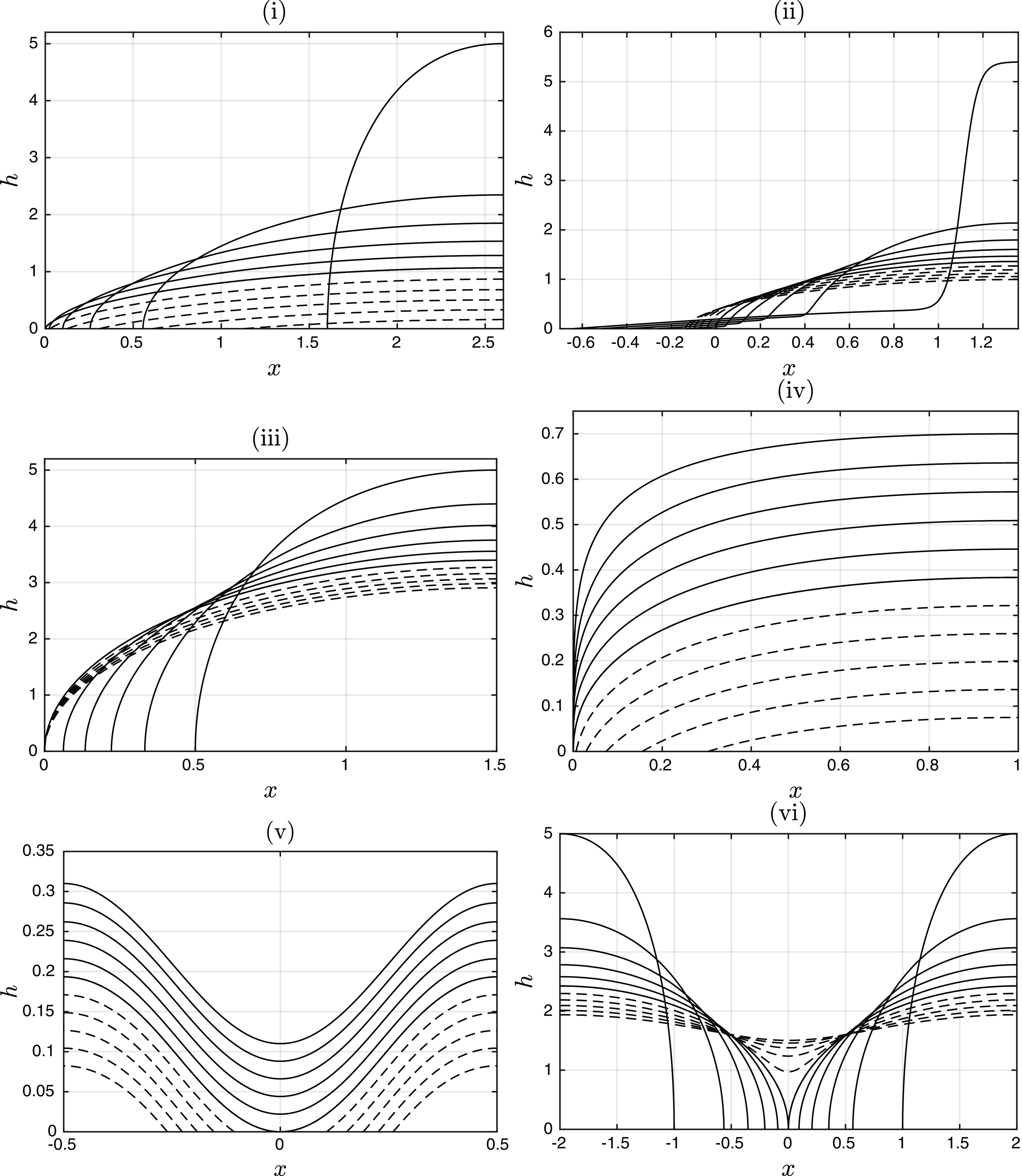
in [Reference Galaktionov and Vazquez11, Reference Galaktionov and Vazquez12]. We shall briefly revisit this phenomena. A sketch of a possible evolution of the compact support in which each of these phenomena is shown schematically in Figure 1, and illustrative numerical solutions local to each of (i)–(vi) are shown in Figure 2.
$0\lt m\lt 1$
in [Reference Galaktionov and Vazquez11, Reference Galaktionov and Vazquez12]. We shall briefly revisit this phenomena. A sketch of a possible evolution of the compact support in which each of these phenomena is shown schematically in Figure 1, and illustrative numerical solutions local to each of (i)–(vi) are shown in Figure 2.
Panels (i)–(vi) show numerical solutions to (1.1) exhibiting reversing, anti-reversing, attaching, detaching, touchdown and coalescence behaviour, respectively. The solid curves indicate snapshots of the solution prior to the event and the dashed curves after the event. A description of the numerical methods used to furnish these solutions is given in Section 8.
Symmetry arguments will play a central role in what follows; see [Reference Bluman and Cole3], for example, for relevant background. For almost all $m$
and
$m$
and $n$
(including all those in the range of interest here), the only continuous symmetries of equation (1.1) are those that are obvious by inspection, namely translations of
$n$
(including all those in the range of interest here), the only continuous symmetries of equation (1.1) are those that are obvious by inspection, namely translations of $x$
and of
$x$
and of $t$
and the scaling invariant
$t$
and the scaling invariant
 \begin{align} h \rightarrow \alpha h, \quad t \rightarrow \alpha^{1-n} t, \quad x \rightarrow \alpha^{(m+1-n)/2} x, \end{align}
for arbitrary constant $\alpha$
. The associated similarity reductions, that is, steady states, spatially uniform solutions, travelling waves and the backward
$\alpha$
. The associated similarity reductions, that is, steady states, spatially uniform solutions, travelling waves and the backward
 \begin{align} h=({-}t)^{\frac{1}{1-n}} f \left (x{({-}t)^{-\frac{m+1-n}{2(1-n)}}} \right ), \end{align}
and forward
 \begin{align} h=t^{\frac{1}{1-n}} f \left ( x{t^{-\frac{m+1-n}{2(1-n)}}} \right ), \end{align}
scaling reductions associated with (1.6), will each play significant roles. The two double reductions
 \begin{align} h=A_* x^{\frac{2}{m+1-n}}, \quad A_* \equiv \left ( \frac{(m+1-n)^2}{2(m+1+n)}\right )^{\frac{1}{m+1-n}}, \end{align}
(both a steady state and a scaling reduction, through (1.7) or (1.8)) and
 \begin{align} h=\left ((1-n) ({-}t) \right )^{\frac{1}{1-n}} \end{align}
(both a spatially uniform solution and a scaling reduction, through (1.7)) play particularly prominent roles.
Other aspects related to symmetry arguments of interest in their own right but of limited relevance to the remainder of the paper are recorded in the Appendix.
Motivation and outline
A specific motivation for the current detailed study is that equation (1.1) is perhaps the simplest PDE to manifest each of the seven classes of singular behaviour noted above. Moreover, Figure 1 is evidently not specific to a particular PDE and the classification is relevant to much more general classes of moving-boundary problem; similarly, the formal-asymptotic methodologies adopted below and their consequences (notably with regard to non-generic, as well as generic, types of singular behaviour) should be of broader applicability, a point that has been recognised in other contexts, notably with regard to blow up.
The aim of the reminder of this paper is to describe the structure of solutions to (1.1) local to an event where an interface (i) reverses, (ii) anti-reverses, (iii) attaches, (iv) detaches, (v) touches down, (vi) coalesces or (vii) goes extinct. Henceforth, we shall assume that the origins of the temporal and spatial coordinates have been defined in such a way that the event of interest occurs at $t=0$
,
$t=0$
, $x=0$
. In Section 2, we discuss the different possible asymptotic behaviours local to both mass-preserving interfaces, satisfying (1.3), and absorbing boundaries, satisfying (1.5). In the subsequent section, Section 3, we examine three scenarios in which (1.1) can be reduced to an ODE namely, (a) when the solution is (quasi-)steady, (b) when the solution takes the form of a travelling wave and (c) when the solution is self-similar. Next, in Section 4, we examine the limiting behaviours in which one of the three terms in (1.1) is negligible. In Section 5, we linearise about (1.9) and (1.10) in order to establish the results needed to characterise the singular behaviours that are not of a ‘pure’ self-similar form. In Section 6, we revisit the self-similar solutions and carry out a detailed analysis of the phase space of the reduced ODE. In Section 7, the results of the preceding sections are leveraged in order to obtain the local behaviour of solutions immediately prior to each of the singular phenomena being investigated. In the penultimate section, Section 8, the asymptotic results are validated against direct numerical simulations of (1.1). Finally, in Section 9, we draw our conclusions.
$x=0$
. In Section 2, we discuss the different possible asymptotic behaviours local to both mass-preserving interfaces, satisfying (1.3), and absorbing boundaries, satisfying (1.5). In the subsequent section, Section 3, we examine three scenarios in which (1.1) can be reduced to an ODE namely, (a) when the solution is (quasi-)steady, (b) when the solution takes the form of a travelling wave and (c) when the solution is self-similar. Next, in Section 4, we examine the limiting behaviours in which one of the three terms in (1.1) is negligible. In Section 5, we linearise about (1.9) and (1.10) in order to establish the results needed to characterise the singular behaviours that are not of a ‘pure’ self-similar form. In Section 6, we revisit the self-similar solutions and carry out a detailed analysis of the phase space of the reduced ODE. In Section 7, the results of the preceding sections are leveraged in order to obtain the local behaviour of solutions immediately prior to each of the singular phenomena being investigated. In the penultimate section, Section 8, the asymptotic results are validated against direct numerical simulations of (1.1). Finally, in Section 9, we draw our conclusions.
As noted above, coalescence and attachment need no further consideration (given that we limit ourselves to the one-dimensional case), and the cases of extinction, reversing and anti-reversing have been the subject of previous analyses. Our specific goals here are to give a comprehensive and, so far as is possible, a unified description of the range of intermediate-asymptotic behaviours shown schematically in Figure 2. In so doing, we address (for the first time) touchdown and detachment, as well as describing novel non-self-similar behaviour of reversing and anti-reversing interfaces. More generally, we seek to illustrate how a combination of self-similar and non-self-similar asymptotic structures provides a framework to analyse broad classes of moving-boundary problems – as already noted, the phenomena shown in Figure 2 are not specific to the PDE in question. That both self-similar and non-self-similar solutions arise in what follows for each scenario in question is also of more general relevance (a point to which we return in Section 9) and requires an analysis of which of the available candidates are generic (i.e. stable) – we undertake such an analysis of (1.1) for the first time.
2. Local behaviour
We now characterise the possible behaviours of (1.1) local to interfaces on which either (1.3) or (1.5) is satisfied, noting that these prove useful in what follows.
Mass-preserving interfaces
Introducing the local variable $\chi$
about the interface
$\chi$
about the interface
 \begin{align} \chi = x-s(t), \end{align}
with, locally, $h\gt 0$
in
$h\gt 0$
in $\chi \gt 0$
and
$\chi \gt 0$
and $h \equiv 0$
in
$h \equiv 0$
in $\chi \lt 0$
and applying the interface conditions (1.3) the following hold
$\chi \lt 0$
and applying the interface conditions (1.3) the following hold
 \begin{align} h^{1-n} \sim \frac{(1-n)}{\dot{s}} \chi \quad \text{as} \quad \chi \to 0^+ \quad \text{provided} \quad \dot{s}\gt 0 \quad (\text{receding interface}), \end{align}
 \begin{align} h^{m} \sim m ({-}\dot{s}) \chi \quad \text{as} \quad \chi \to 0^+ \quad \text{provided} \quad \dot{s}\lt 0 \quad (\text{advancing interface}). \end{align}
The former requires that the second term in (1.1) be negligible in the limit, which, in turn, implies
 \begin{align} n \lt 1, \quad m+n \gt 1. \end{align}
The latter, (2.3), requires that the third term in (1.1) be negligible in the limit, implying that
 \begin{align} m\gt 0, \quad m + n \gt 1. \end{align}
Absorbing boundaries
On imposing (1.5), $h|_{x=0}=0$
, the apparent sole candidate for the local behaviour neglects both the first and the third term in (1.1), and is
$h|_{x=0}=0$
, the apparent sole candidate for the local behaviour neglects both the first and the third term in (1.1), and is
 \begin{align} h^{m+1} \sim (m+1) J x \quad \text{as} \quad x \searrow 0, \end{align}
where $J(t)\gt 0$
is the flux through the boundary at
$J(t)\gt 0$
is the flux through the boundary at $x=0$
. Here self-consistency requires
$x=0$
. Here self-consistency requires $m\gt -1$
and
$m\gt -1$
and $m+n\gt -1$
, a condition that is automatically satisfied by our prior imposition of (1.2).
$m+n\gt -1$
, a condition that is automatically satisfied by our prior imposition of (1.2).
Each of the expressions (2.2), (2.3) and (2.6) contains a single degree of freedom ( $s$
or
$s$
or $J$
), as required for a second-order PDE; this conclusion is near-immediate for (2.3) and (2.6), while for (2.2) it requires an application of the Liouville-Green (JWKB) method.
$J$
), as required for a second-order PDE; this conclusion is near-immediate for (2.3) and (2.6), while for (2.2) it requires an application of the Liouville-Green (JWKB) method.
3. Exact reductions to the PDE
Standard symmetry methods imply that there are three scenarios in which the PDE (1.1) can be reduced to an ODE, namely steady states, travelling waves and scaling self-similarity.
3.1. Steady states
The steady-state solutions to (1.1) satisfy
 \begin{align} \frac{d}{dx} \left (h^m \frac{d h}{d x} \right ) = h^n, \end{align}
an ODE that will subsequently arise as a quasi-steady balance in (1.1) for circumstances in which the time derivative is non-zero but negligible. On integrating with respect to $x$
, we have that
$x$
, we have that
 \begin{align} \frac{1}{2} h^{2m} \left ( \frac{dh}{dx} \right )^2 = \frac{1}{m+n+1} h^{m+n+1} + C_1, \end{align}
for arbitrary constant $C_1$
. Given the scaling invariance of (3.1),
$C_1$
. Given the scaling invariance of (3.1),
 \begin{align} x \mapsto \phi^{m-n+1} x, \quad h \mapsto \phi ^2 h, \end{align}
where $\phi$
is an arbitrary constant, we may scale
$\phi$
is an arbitrary constant, we may scale $|C_1|$
in (3.2) to a convenient value. In this section, we shall set
$|C_1|$
in (3.2) to a convenient value. In this section, we shall set $C_1=0$
,
$C_1=0$
, $C_1=1/2$
and
$C_1=1/2$
and $C_1=-1/(m+n+1)$
in turn. Given (3.3), these zero, positive and negative values in effect cover the full range of possibilities, the specific values being chosen for algebraic convenience in the sense of (3.7) and (3.9) below.
$C_1=-1/(m+n+1)$
in turn. Given (3.3), these zero, positive and negative values in effect cover the full range of possibilities, the specific values being chosen for algebraic convenience in the sense of (3.7) and (3.9) below.


The exceptional solution
For $C_1=0$
, we have the steady solution (1.9), up to translational invariance. In Sections 3.3, 5 and 6, we shall see that it is a common component of a host of relevant solutions; owing to its significance in the remainder of the analysis, we shall refer to it as the ‘exceptional solution’. Linearising (3.2) about (1.9), we obtain
$C_1=0$
, we have the steady solution (1.9), up to translational invariance. In Sections 3.3, 5 and 6, we shall see that it is a common component of a host of relevant solutions; owing to its significance in the remainder of the analysis, we shall refer to it as the ‘exceptional solution’. Linearising (3.2) about (1.9), we obtain
 \begin{align} h \sim A_* x^{\alpha } + \nu _1 x^{\alpha -1} + \nu _2 x^{-(m+n)\alpha } \end{align}
where
 \begin{align} \alpha =\frac{2}{m+1-n}. \end{align}
The $\nu _1$
term in (3.4) reflects translational invariance in
$\nu _1$
term in (3.4) reflects translational invariance in $x$
and is less singular as
$x$
and is less singular as $x \rightarrow 0$
than the
$x \rightarrow 0$
than the $\nu _2$
term when
$\nu _2$
term when $m+3n+1\gt 0$
, a condition that we impose throughout.
$m+3n+1\gt 0$
, a condition that we impose throughout.
The leaking solution
Setting $C_1=1/2$
in (3.2) and imposing the interface condition (1.5) gives
$C_1=1/2$
in (3.2) and imposing the interface condition (1.5) gives
 \begin{align} \frac{1}{2} h^{2m} \left ( \frac{dh}{dx} \right )^2 = \frac{1}{m+n+1} h^{m+n+1} + \frac{1}{2}, \quad h|_{x=0}=0. \end{align}
A numerical solution is shown in yellow in Figure 3. This solution, which we shall refer to as the ‘leaking solution’, has a unit outward flux through the origin, that is, it has the property
 \begin{align} \left. h^m \frac{dh}{dx} \right |_{x=0} = 1, \end{align}
and is a candidate to form part of the asymptotic description of a solution to (1.1) that is attached to an absorbing boundary. The solution to (3.6) has asymptotic behaviour given by (3.4) as $x \to +\infty$
, with
$x \to +\infty$
, with $\nu _1$
and
$\nu _1$
and $\nu _2$
depending on
$\nu _2$
depending on $m$
and
$m$
and $n$
, the
$n$
, the $\nu _1$
term being the dominant correction term for
$\nu _1$
term being the dominant correction term for $m+3n+1\gt 0$
. For
$m+3n+1\gt 0$
. For $n=0$
, we have the explicit solution
$n=0$
, we have the explicit solution
 \begin{align*} \frac{1}{m+1} h^{m+1} =\frac{1}{2} x^2 +x. \end{align*}
The pre-touchdown solution
Finally, setting $C_1=-1/(m+n+1)$
in (3.2) and imposing a boundary condition that requires the solution to have zero gradient at the origin leads to
$C_1=-1/(m+n+1)$
in (3.2) and imposing a boundary condition that requires the solution to have zero gradient at the origin leads to
 \begin{align} \frac{1}{2} h^{2m} \left ( \frac{dh}{dx} \right )^2 = \frac{1}{m+n+1}\left ( h^{m+n+1} -1 \right ), \quad \left. \frac{dh}{dx} \right |_{x=0} = 0. \end{align}
The solution to this problem (determined numerically) is shown in green in Figure 3. We shall refer to this solution as the ‘pre-touchdown solution’, and it has the property
 \begin{align} h|_{x=0} = 1. \end{align}
This solution, scaled by an appropriate function of time (i.e. in quasi-steady form), will play a role in the pre-touchdown dynamics. Once again, the solution (3.8) has the far-field behaviour (3.4). In the case $n=0$
, it has explicit solution
$n=0$
, it has explicit solution
 \begin{align*} \frac{1}{m+1} h^{m+1} =\frac{1}{2} x^2 +\frac{1}{m+1}. \end{align*}
Exceptionally, the far-field behaviour of (3.8) has $\nu _1=0$
in (3.4) when
$\nu _1=0$
in (3.4) when $n=0$
. For
$n=0$
. For $n\lt 0$
, we have
$n\lt 0$
, we have $\nu _1 \lt 0$
in (3.4) while for
$\nu _1 \lt 0$
in (3.4) while for $n\gt 0$
we have
$n\gt 0$
we have $\nu _1 \gt 0$
; this has implications for the intermediate-asymptotic behaviour. More precisely,
$\nu _1 \gt 0$
; this has implications for the intermediate-asymptotic behaviour. More precisely,
 \begin{align} h^{\frac{m+1-n}{2}} \sim \frac{m+1-n}{(2(m+n+1))^{1/2}} x + \frac{n}{m+n+1} B \left ( \frac{1}{2}, \frac{m+3n+1}{2(m+n+1)} \right ) \quad \text{as} \quad x \to + \infty, \end{align}
where $B$
denotes the beta function and the constraint
$B$
denotes the beta function and the constraint $m+3n+1\gt 0$
again rears its head.
$m+3n+1\gt 0$
again rears its head.
3.2. Travelling-wave solutions
Here we consider travelling-wave solutions to (1.1),
 \begin{align} h=h(\zeta ), \qquad \zeta =x- v t, \end{align}
where the constant $v \neq 0$
is the wave speed. Substitution of (3.11) into (1.1) yields the ODE
$v \neq 0$
is the wave speed. Substitution of (3.11) into (1.1) yields the ODE
 \begin{align} -v\frac{ d h}{d \zeta }=\frac{ d }{d \zeta }\left ({h}^m \frac{ d h}{d \zeta } \right )-{h}^n. \end{align}
We shall require a solution that satisfies (1.3) at $\zeta =0$
, so that
$\zeta =0$
, so that
 \begin{align} h|_{\zeta =0}=0, \qquad \left. h^m \frac{\partial h}{\partial \zeta } \right |_{\zeta =0}=0. \end{align}
Subsequently, for solutions with a moving interface, $v$
will be identified with
$v$
will be identified with $\dot{s}$
, with the travelling-wave balance (3.12), again in quasi-steady form, providing the local behaviour about the interface whenever
$\dot{s}$
, with the travelling-wave balance (3.12), again in quasi-steady form, providing the local behaviour about the interface whenever $\dot{s}\neq 0$
.
$\dot{s}\neq 0$
.
Via the rescalings
 \begin{align} h \to |v|^{\frac{2}{m+n-1}} h, \qquad \zeta \to |v|^{\frac{m+1-n}{m+n-1}} \zeta \end{align}
we can without loss of generality set $v=\pm 1$
in (3.12). The phase plane for an advancing interface (
$v=\pm 1$
in (3.12). The phase plane for an advancing interface ( $v\lt 0$
) is plotted in Figure 4 panel (a). The initial conditions (3.13) correspond to the sole trajectory that emanates from the origin, the asymptotic behaviour of which is given in terms of the unscaled variables by
$v\lt 0$
) is plotted in Figure 4 panel (a). The initial conditions (3.13) correspond to the sole trajectory that emanates from the origin, the asymptotic behaviour of which is given in terms of the unscaled variables by
 \begin{align} h \sim \left (({-}v) m \zeta \right )^{1/m} \quad \mbox{as} \quad \zeta \to 0^+ \quad \text{with} \quad v\lt 0, \end{align}
corresponding to the local behaviour (2.3). The phase plane for $v\gt 0$
(a receding interface) is plotted in Figure 4 panel (b). The conditions (3.13) are associated with the sole trajectory that emanates from the origin, the unscaled version of which satisfies
$v\gt 0$
(a receding interface) is plotted in Figure 4 panel (b). The conditions (3.13) are associated with the sole trajectory that emanates from the origin, the unscaled version of which satisfies
 \begin{align} h \sim \left (\frac{(1-n)}{v} \zeta \right )^{1/(1-n)} \quad \mbox{as} \quad{\zeta \rightarrow 0^+} \quad \text{with} \quad v\gt 0. \end{align}
coinciding with (2.2).
Phase planes for (a) the advancing ( $v\lt 0$
) and (b) the receding (
$v\lt 0$
) and (b) the receding ( $v\gt 0$
) travelling waves. Here
$v\gt 0$
) travelling waves. Here $m=3$
and
$m=3$
and $n=0$
, but qualitatively similar results apply for other exponents in the range (1.2). The red curves indicate the trajectories leaving the origin and corresponding to the solution which links the behaviours (3.15) and (3.17) in panel (a), and (3.16) and (3.17) in panel (b). Since
$n=0$
, but qualitatively similar results apply for other exponents in the range (1.2). The red curves indicate the trajectories leaving the origin and corresponding to the solution which links the behaviours (3.15) and (3.17) in panel (a), and (3.16) and (3.17) in panel (b). Since $v \to -v$
results from
$v \to -v$
results from $\zeta \to -\zeta$
in (3.12), (a) and (b) can be viewed as upper and lower quadrants of the same phase plane on also swapping the direction of the trajectories in one case. All the trajectories have the same far-field behaviour, (3.18).
$\zeta \to -\zeta$
in (3.12), (a) and (b) can be viewed as upper and lower quadrants of the same phase plane on also swapping the direction of the trajectories in one case. All the trajectories have the same far-field behaviour, (3.18).

Far-field behaviour
The phase-plane analysis demonstrates that both advancing and receding interfaces have the same far-field behaviour, with the left-hand side of (3.12) being negligible at leading order, so that
 \begin{align} h \sim A_* \zeta^{\alpha } \quad \mbox{as} \quad \zeta \rightarrow +\infty. \end{align}
We shall need a more detailed description of the behaviour; however, the relevant correction terms follow from (3.4) and from the left-hand side of (3.12) and result in the far-field behaviour
 \begin{align} h \sim A_* \zeta ^\alpha - v B \zeta^{\alpha -\beta } + \nu _1\zeta^{\alpha -1} + \nu _2 \zeta^{-(m+n)\alpha } \quad \text{as} \quad \zeta \to +\infty, \end{align}
where the constants $\beta$
and
$\beta$
and $B$
are given by
$B$
are given by
 \begin{align} \beta =\frac{m+n-1}{m+1-n}, \quad B= \frac{(2(m+n+1))^{\frac{m-1}{m+1-n}}(m+1-n)^{\frac{3-m-n}{m+1-n}}}{(1-n) (n+m+3)}. \end{align}
The $B$
term is the dominant correction term in (3.18), given the condition (1.2), while
$B$
term is the dominant correction term in (3.18), given the condition (1.2), while $\nu _1$
and
$\nu _1$
and $\nu _2$
are the requisite two degrees of freedom. The phase planes confirm that the IVP (3.12)–(3.13) has a unique solution for given
$\nu _2$
are the requisite two degrees of freedom. The phase planes confirm that the IVP (3.12)–(3.13) has a unique solution for given $v$
,
$v$
, $m$
and
$m$
and $n$
; the dependencies of
$n$
; the dependencies of $\nu _1$
and
$\nu _1$
and $\nu _2$
upon
$\nu _2$
upon $v$
can be inferred from the above noted scaling property, their dependence on
$v$
can be inferred from the above noted scaling property, their dependence on $m$
and
$m$
and $n$
depending on the sign of
$n$
depending on the sign of $v$
.
$v$
.
In the light of these properties, and in the parameter range (1.2), the velocity of the travelling wave can thus be determined if the coefficient of the third term in far-field behaviour (3.18) is known, this being the dominant correction term in (3.18), since $\beta \gt 1$
.
$\beta \gt 1$
.
3.3. Self-similar solutions
As we shall see below, the backward self-similar reduction for (1.1),
 \begin{align} h(x,t) = \left ({-}t \right )^{\frac{1}{1-n}} \; f(\xi ), \quad \xi = x ({-}t)^{-\frac{m+1-n}{2(1-n)}} \quad \mbox{for} \quad t \lt 0, \end{align}
coupled to the free and absorbing boundary conditions (1.3) and (1.5), provides a plausible scenario for times leading up to a singular event. As in [Reference Foster, Please, Fitt and Richardson7], substituting (3.20) into (1.1) reveals that $f$
satisfies the ODE
$f$
satisfies the ODE
 \begin{align} \frac{1}{1-n} \left ({-} f + \frac{m+1-n}{2} \, \xi \frac{d f}{d \xi } \right ) = \frac{d}{d \xi } \left ( f^m \frac{d f}{d \xi } \right ) - f^n. \end{align}
The power-law solution to (3.21) is the exceptional solution (1.9), which in similarity variables reads
 \begin{align} f = A_* \xi^{\alpha }. \end{align}
As a precursor to constructing solutions to (3.21) which give rise to dynamic interfaces, it is helpful to examine the possible near-field behaviours of $f$
about the interface at
$f$
about the interface at $\xi = \hat{\xi }$
. We find that
$\xi = \hat{\xi }$
. We find that
 \begin{align} f \sim \left ( \frac{m (m+1-n) \hat{\xi }}{2 (1-n)} (\xi - \hat{\xi }) \right )^{1/m} \quad \textrm{as} \quad \xi \to \hat{\xi }^+ \quad \mbox{for} \quad \hat{\xi } \gt 0, \end{align}
 \begin{align} f \sim \left ( \frac{2 (1-n)^2}{(m+1-n)({-}\hat{\xi })} (\xi - \hat{\xi }) \right )^{1/(1-n)} \quad \textrm{as} \quad \xi \to \hat{\xi }^+ \quad \mbox{for} \quad \hat{\xi } \lt 0 \end{align}
are admissible. Here, $\hat{\xi } \neq 0$
is a free parameter. In the context of the original PDE, (1.1), the former behaviour corresponds to an advancing interface with
$\hat{\xi } \neq 0$
is a free parameter. In the context of the original PDE, (1.1), the former behaviour corresponds to an advancing interface with $\dot{s}\lt 0$
(as, e.g., depicted by the solid curves in Figure 2(i), which show an advancing solution before reversing), while the latter corresponds to a receding interface with
$\dot{s}\lt 0$
(as, e.g., depicted by the solid curves in Figure 2(i), which show an advancing solution before reversing), while the latter corresponds to a receding interface with $\dot{s}\gt 0$
. The behaviours (3.23)–(3.24) correspond to (2.2)–(2.3). In [Reference Foster, Gysbers, King and Pelinovsky5–Reference Foster, Please, Fitt and Richardson7], the Liouville-Green method was used (which involves linearising about (3.23) in (3.21) and examining the self-consistent asymptotic behaviours) to demonstrate that there is only one degree of freedom in both of these behaviours, namely
$\dot{s}\gt 0$
. The behaviours (3.23)–(3.24) correspond to (2.2)–(2.3). In [Reference Foster, Gysbers, King and Pelinovsky5–Reference Foster, Please, Fitt and Richardson7], the Liouville-Green method was used (which involves linearising about (3.23) in (3.21) and examining the self-consistent asymptotic behaviours) to demonstrate that there is only one degree of freedom in both of these behaviours, namely $\hat{\xi }$
.
$\hat{\xi }$
.
Even solutions satisfying
 \begin{align} f \sim \hat{f} + \frac{1}{2} \hat{f}^{-m} \left (\hat{f}^n-\frac{1}{1-n} \hat{f} \right ) \xi ^2 \quad \mbox{as} \quad \xi \to 0, \end{align}
wherein $\hat{f}\gt 0$
is the sole free parameter, are also of potential relevance. This behaviour clearly does not correspond to an interface of (1.1) but, in time-dependent setting, it corresponds to a point of no flux and is a candidate to describe a solution leading up to a touchdown event.
$\hat{f}\gt 0$
is the sole free parameter, are also of potential relevance. This behaviour clearly does not correspond to an interface of (1.1) but, in time-dependent setting, it corresponds to a point of no flux and is a candidate to describe a solution leading up to a touchdown event.
A fourth alternative is
 \begin{align} f \sim K \xi^{1/(m+1)} \quad \mbox{as} \quad \xi \to 0^+, \end{align}
where $K\gt 0$
is the sole free parameter. This leads to a static interface of (1.1) through which mass is being lost (as, e.g., depicted by the solid ones in 2(iv)). There is a final near-field behaviour of relevance, namely the exceptional solution (1.9); in view of (3.4), this contains no degrees of freedom.
$K\gt 0$
is the sole free parameter. This leads to a static interface of (1.1) through which mass is being lost (as, e.g., depicted by the solid ones in 2(iv)). There is a final near-field behaviour of relevance, namely the exceptional solution (1.9); in view of (3.4), this contains no degrees of freedom.
The only relevant far-field behaviour for solutions to (3.21) is
 \begin{equation} f \sim A \xi^{\alpha } \quad \mbox{as} \quad \xi \to +\infty, \end{equation}
and it has been shown in [Reference Foster, Please, Fitt and Richardson7] that the parameter $A\gt 0$
is the only degree of freedom in the large
$A\gt 0$
is the only degree of freedom in the large $\xi$
behaviour. Unpicking the transformation to the self-similar variables, (3.27) corresponds to
$\xi$
behaviour. Unpicking the transformation to the self-similar variables, (3.27) corresponds to
 \begin{align} h \sim A x^\alpha \end{align}
and is a candidate for the local behaviour as $x \to 0^+$
of the solution at
$x \to 0^+$
of the solution at $t=0$
, given that
$t=0$
, given that $\xi \to + \infty$
as
$\xi \to + \infty$
as $t \to 0^-$
at fixed
$t \to 0^-$
at fixed $x$
. We note that (3.27) coincides with the exceptional solution (1.9) in the case when
$x$
. We note that (3.27) coincides with the exceptional solution (1.9) in the case when $A=A_*$
. We shall return in Section 6 to a detailed exploration of these self-similar forms.
$A=A_*$
. We shall return in Section 6 to a detailed exploration of these self-similar forms.
4. Limiting cases of the PDE
Here we examine the properties (in particular, the similarity solutions) of solutions in the limiting cases in which one of the three terms in (1.1) is negligible. There are three scenarios. First, where the time derivative is negligible and the solutions are quasi-steady; the results of Section 3.1 then apply. In this section, we cover the other two cases, namely where the sink term is negligible, and where the diffusion term is negligible. Section 5 is devoted to a different class of limiting behaviour that will also prove relevant, namely linearisation about the uniform state and about the exceptional power-law solution.
4.1. Porous-medium equation balance
Neglecting the sink term in (1.1) gives the so-called porous-medium equation, that is,.
 \begin{align} \frac{\partial h}{\partial t} \sim \frac{\partial }{\partial x} \left (h^m \frac{\partial h}{\partial x} \right ) \end{align}
the similarity solutions of which (as well as its other properties) have been very widely investigated, see, for example, [Reference Lacey, Ockendon and Tayler21]. We potentially need both the backward ( $t\lt 0$
) self-similar solutions
$t\lt 0$
) self-similar solutions
 \begin{align} h \sim ({-}t)^\nu f_-(\eta _-), \quad \eta _- = x ({-}t)^{-\frac{m\nu +1}{2}} \quad \text{as} \quad t \to 0^- \quad \text{with} \quad \eta _-=O(1) \end{align}
and the forward ( $t\gt 0$
) ones
$t\gt 0$
) ones
 \begin{align} h \sim t^\nu f_+(\eta _+), \quad \eta _+ = x t^{-\frac{m \nu +1}{2}} \quad \text{as} \quad t \to 0^+ \quad \text{with} \quad \eta _+=O(1). \end{align}
The case $\nu =1/m$
is of most significance to us for reasons that will become clear later: in this case
$\nu =1/m$
is of most significance to us for reasons that will become clear later: in this case
 \begin{align*} f_-^m = m\hat{\eta }( \eta _- -\hat{\eta })_+, \qquad f_+^m = m\hat{\eta }( \eta _- + \hat{\eta })_+ \end{align*}
for some constant $\hat{\eta }$
; these are each both a scaling reduction and a travelling-wave solution to (4.1) and represent an exceptional connection in the phase space of
$\hat{\eta }$
; these are each both a scaling reduction and a travelling-wave solution to (4.1) and represent an exceptional connection in the phase space of $f_-$
– see [Reference Hulshof, King and Bowen14]. Neglect of the
$f_-$
– see [Reference Hulshof, King and Bowen14]. Neglect of the $h^n$
terms as
$h^n$
terms as $|t| \to 0$
requires, for legitimacy, that
$|t| \to 0$
requires, for legitimacy, that
 \begin{align} \nu \lt 1/(1-n), \end{align}
which in the case $\nu =1/m$
implies that
$\nu =1/m$
implies that $m+n\gt 1$
, consistent with (1.2).
$m+n\gt 1$
, consistent with (1.2).
4.2. Absorption balance
The last of the three possible balances in which one of the terms in (1.1) is entirely neglected is
 \begin{align} \frac{\partial h}{\partial t} \sim - h^n \end{align}
so that
 \begin{align} h^{1-n} \sim h_0^{1-n}(x) + (1-n) ({-}t). \end{align}
Here, $h_0(x)$
is an arbitrary function. As we shall see, the balance (4.5) can play an asymptotic role for power law
$h_0(x)$
is an arbitrary function. As we shall see, the balance (4.5) can play an asymptotic role for power law
 \begin{align} h_0(x) = M |x|^{\mu/(1-n)} \end{align}
for positive constants $M$
and
$M$
and $\mu$
. In such instances, it is instructive to interpret (4.6) as backward and forward similarity reductions,
$\mu$
. In such instances, it is instructive to interpret (4.6) as backward and forward similarity reductions,
 \begin{align} h = ({-}t)^{\frac{1}{1-n}} g_-(\omega _-), \quad \omega _- = x ({-}t)^{-1/\mu }, \quad g_-^{1-n} = M^{1-n} |\omega _-|^{\mu } + (1-n), \end{align}
 \begin{align} h = t^{\frac{1}{1-n}} g_+(\omega _+), \quad \omega _+ = x t^{-1/\mu }, \quad g_+^{1-n} = M^{1-n} |\omega _+|^{\mu } - (1-n), \end{align}
from which it is clear that self-consistency as $|t| \to 0$
in the neglect of the diffusion term in (1.1) requires
$|t| \to 0$
in the neglect of the diffusion term in (1.1) requires
 \begin{align} \mu m + (\mu -2) (1-n)\gt 0. \end{align}
5. Linearisations
In this section, we linearise about two special solutions to (1.1), namely the uniform solution (1.10) and exceptional power-law solution (1.9). The analysis of Section 7 is devoted to characterising which of the possible candidates identified in Sections 3 –6 can in fact be realised in describing the various types of singular behaviour.
5.1. Linearisation about the uniform state
We linearise about the uniform state, (1.10), by setting
 \begin{align} h \sim \left ( (1-n)({-}t) \right )^{1/(1-n)} +{\mathcal H}(x,t) \end{align}
in (1.1) and neglect nonlinear terms in $\mathcal H$
to give
$\mathcal H$
to give
 \begin{align} \frac{\partial{\mathcal H}}{\partial t} = \left ( (1-n)({-}t) \right )^{m/(1-n)} \frac{\partial ^2{\mathcal H}}{\partial x^2} - \frac{n}{(1-n)({-}t)}{\mathcal H}. \end{align}
Defining
 \begin{align}{\mathcal H} = ({-}t)^{\frac{n}{1-n}}{\mathcal G}(x,\tau ), \quad -\tau = \frac{((1-n)({-}t))^{\frac{m+1-n}{1-n}}}{m+1-n} \end{align}
transforms (5.2) to the heat equation
 \begin{align} \frac{\partial{\mathcal G}}{\partial \tau } = \frac{\partial ^2{\mathcal G}}{\partial x^2}. \end{align}
The backward self-similar solutions without exponential growth as $|x| \to +\infty$
are given by the Hermite polynomials
$|x| \to +\infty$
are given by the Hermite polynomials $H_k$
, namely
$H_k$
, namely
 \begin{align}{\mathcal G} = C_k ({-}\tau )^{k/2} H_k \left ( x ({-}\tau )^{-1/2}/ 2 \right ) \end{align}
where $k$
is a non-negative integer and
$k$
is a non-negative integer and $C_k$
is some constant.Footnote 2
$C_k$
is some constant.Footnote 2
The following properties will be needed in due course. Firstly, (5.3)–(5.5) require, for the self-consistency of (5.1) (i.e. that the second term therein be negligible in comparison to the first in the limit that $t \rightarrow 0^-$
), that
$t \rightarrow 0^-$
), that
 \begin{align} km + (k-2)(1-n)\gt 0; \end{align}
the case $k=0$
is therefore always excluded, unsurprisingly since it simply corresponds to a translation in
$k=0$
is therefore always excluded, unsurprisingly since it simply corresponds to a translation in $t$
. Secondly, a standard result for
$t$
. Secondly, a standard result for $H_k$
implies that (5.5) renders the matching condition
$H_k$
implies that (5.5) renders the matching condition
 \begin{align}{\mathcal H}(x,t) \sim C_k ({-}t)^{-\frac{n}{1-n}} x^k \quad \text{as} \quad | x ({-}\tau )^{-1/2} | \to \infty, \end{align}
so that
 \begin{align} h^{1-n} \sim (1-n)({-}t) + (1-n)^{\frac{1-2n}{1-n}} C_k x^k, \end{align}
5.2. Linearisation about the exceptional solution
The other linearised problem that we shall need to characterise is that about the exceptional solution, (1.9). On setting
 \begin{align} h \sim A_* x^{\alpha } + \bar{\mathcal H}(x,t) \end{align}
in (1.1), linearising in $\bar{\mathcal H}$
gives
$\bar{\mathcal H}$
gives
 \begin{align} \frac{\partial \bar{\mathcal H}}{\partial t} = A_*^m \frac{\partial ^2}{\partial x^2} \left ( x^{m \alpha } \bar{\mathcal H} \right )- n A_*^{-(1-n)} x^{-(1-n) \alpha } \bar{\mathcal H}. \end{align}
Elucidating the behaviour of solutions to (5.10) will provide information crucial to what follows, specifically with regard to backward self-similarity. In order to analyse the linear problem (5.10), it is helpful to use the definitions of $A_*$
and
$A_*$
and $\alpha$
to rewrite it in the form
$\alpha$
to rewrite it in the form
 \begin{align} x^{2-m \alpha } \frac{\partial \bar{\mathcal H}}{\partial t} = A_*^m \left ( x^{2-m \alpha } \frac{\partial ^2}{\partial x^2} \left ( x^{m \alpha } \bar{\mathcal H} \right )- (\alpha (m+1)-2)(\alpha (m+1)-1) \bar{\mathcal H} \right ). \end{align}
The right-hand side of (5.11) dominates as $x \rightarrow 0$
, since
$x \rightarrow 0$
, since $2-m\alpha \gt 0$
in the range of parameters that we consider, (1.2). The possible solution behaviours are thus found by neglecting the left-hand side of (5.11) and solving the resulting Euler equation in
$2-m\alpha \gt 0$
in the range of parameters that we consider, (1.2). The possible solution behaviours are thus found by neglecting the left-hand side of (5.11) and solving the resulting Euler equation in $x$
for
$x$
for $\bar{\mathcal H}$
; these are
$\bar{\mathcal H}$
; these are
 \begin{align} \bar{\mathcal H} \sim \nu _1(t) x^{\alpha -1}, \qquad \bar{\mathcal H} \sim \nu _2(t) x^{-(m+n)\alpha }, \end{align}
where $\nu _1(t)$
and
$\nu _1(t)$
and $\nu _2(t)$
are arbitrary functions, as in (3.4). There are two distinct cases to be considered: for
$\nu _2(t)$
are arbitrary functions, as in (3.4). There are two distinct cases to be considered: for $m+3n +1\gt 0$
, the second of (5.12) is the more singular so it is natural to specify
$m+3n +1\gt 0$
, the second of (5.12) is the more singular so it is natural to specify
 \begin{align} \bar{\mathcal H}=o\left ( x^{-(2m+1)\alpha +2} \right ) \quad \mbox{as} \quad x \to 0^+ \quad \mbox{if} \quad m+3n +1\gt 0 \end{align}
as a boundary condition on (5.10), the local behaviour then being given by the first of (5.12), corresponding to a (small) translation of $x$
in (5.9). By contrast, if
$x$
in (5.9). By contrast, if $m+3n +1\lt 0$
the first of (5.12) is the more singular so it is natural instead to specify
$m+3n +1\lt 0$
the first of (5.12) is the more singular so it is natural instead to specify
 \begin{align} \bar{\mathcal H}=o\left ( x^{\alpha -1}\right ) \quad \mbox{as} \quad x \to 0^+ \quad \mbox{if} \quad m+3n +1\lt 0. \end{align}
As already noted, henceforth we only consider the case $m+3n +1\gt 0$
, so that (5.13) applies (though in (II) below we record an instructive result for
$m+3n +1\gt 0$
, so that (5.13) applies (though in (II) below we record an instructive result for $m+3n+1\lt 0$
); the analysis of the converse case proceeds on similar lines, but will be omitted here (in part because it appears of less physical relevance).
$m+3n+1\lt 0$
); the analysis of the converse case proceeds on similar lines, but will be omitted here (in part because it appears of less physical relevance).
Two transformations, (I) and (II) below, reduce (5.10) to standard forms. In both cases, we define
 \begin{align} r = x^{\frac{2-m \alpha }{2}}, \end{align}
the definitions of $G_i$
being guided by (5.12). We have
$G_i$
being guided by (5.12). We have
 \begin{align} \text{(I): } \quad \bar{\mathcal H}(x,t) = x^{\alpha -1} G_1(r,t), \quad m+3n+1\gt 0, \end{align}
 \begin{align} \frac{\partial G_1}{\partial t} = \frac{1}{4} (2-m \alpha )^2 A_*^m \left ( \frac{\partial ^2 G_1}{\partial r^2} + \frac{N_1 - 1}{r} \frac{\partial G_1}{\partial r} \right ), \quad N_1 = 2\frac{(m+2)\alpha - 1}{2-m \alpha }. \end{align}
 \begin{align} \text{(II): } \quad \bar{\mathcal H}(x,t) = x^{-(m+n)\alpha } G_2(r,t), \quad m+3n+1\lt 0, \end{align}
 \begin{align} \frac{\partial G_2}{\partial t} = \frac{1}{4} (2-m\alpha )^2 A_*^m \left ( \frac{\partial G_2}{\partial r^2} + \frac{N_2 - 1}{r} \frac{\partial G_2}{\partial r} \right ), \quad N_2= 2\frac{5-(3m+2)\alpha }{2-m \alpha }. \end{align}
These representations allow application of standard theory for the radially symmetric heat equation.Footnote 3 As was pursued in [Reference Foster, Gysbers, King and Pelinovsky5], the standard forms for the backward similarity solutions to (5.17) and (5.19) are
 \begin{align} G = ({-}t)^M g(y), \quad y = \frac{2 r}{ A_*^{m/2} (2-m \alpha ) ({-}t)^{1/2}} \end{align}
(where $M$
is an arbitrary constant) and satisfy
$M$
is an arbitrary constant) and satisfy
 \begin{align} z \frac{d^2 g}{d z^2} + \left ( \frac{N}{2} - z \right ) \frac{dg}{dz} + Mg=0, \quad z = y^2, \end{align}
so that the solutions having the necessary regularity as $z \to 0$
(namely
$z \to 0$
(namely $g$
finite as
$g$
finite as $z \to 0$
) and growing algebraically, rather than exponentially (of the form
$z \to 0$
) and growing algebraically, rather than exponentially (of the form $\log g \sim z$
as
$\log g \sim z$
as $z \to +\infty$
), as
$z \to +\infty$
), as $z \to +\infty$
are given by the generalised Laguerre polynomials,
$z \to +\infty$
are given by the generalised Laguerre polynomials,
 \begin{align} g \propto L_P^{(N-2)/2} (z), \end{align}
where $P = M + (N-2)/2$
; since
$P = M + (N-2)/2$
; since $(N-2)/2$
need not be an integer, this is not the standard case, but
$(N-2)/2$
need not be an integer, this is not the standard case, but $M$
is required to be a positive integer, leading to
$M$
is required to be a positive integer, leading to $g$
being an
$g$
being an $M$
-th order polynomial in
$M$
-th order polynomial in $z$
(i.e. in (5.20)–(5.21),
$z$
(i.e. in (5.20)–(5.21), $M$
should be viewed as an eigenvalue, leading to the requirement that it be a non-negative integer). The first few eigenmodes (radially symmetric heat polynomials, representing a complete set of eigenmodes) are thus multiples of the following:
$M$
should be viewed as an eigenvalue, leading to the requirement that it be a non-negative integer). The first few eigenmodes (radially symmetric heat polynomials, representing a complete set of eigenmodes) are thus multiples of the following:
 \begin{align} M = 0, \quad g_0 = 1, \end{align}
 \begin{align} M = 1, \quad g_1 = z - N/2, \end{align}
 \begin{align} M = 2, \quad g_2 = z^2-(N+2)z+N(N+2)/4, \end{align}
 \begin{align} M=3, \quad g_3 = z^3 - 3(N+4)z^2/2 + 3 (N+2)(N+4)z/4 - N(N+2)(N+4)/8. \end{align}
We shall subsequently need to view the leading term in (5.9) as a similarity solution of the form (4.9), while in case (I) above (5.20) implies that $\bar{\mathcal H}$
is of the self-similar form
$\bar{\mathcal H}$
is of the self-similar form
 \begin{align} \bar{\mathcal H} = ({-}t)^L F(\xi ), \quad \text{where} \quad L = M+\frac{1+n-m}{2(1-n)}, \end{align}
so self-consistency of (5.9) requires that
 \begin{align} M \gt \frac{m+1-n}{2(1-n)}. \end{align}
Hence, $M=0$
and
$M=0$
and $M=1$
are excluded (in the latter case (5.28) would require
$M=1$
are excluded (in the latter case (5.28) would require $m+n\lt 1$
for
$m+n\lt 1$
for $n\lt 1$
, again identifying familiar borderline cases). This is to be expected in view of the invariance of (1.1) under translations of
$n\lt 1$
, again identifying familiar borderline cases). This is to be expected in view of the invariance of (1.1) under translations of $x$
and
$x$
and $t$
, illustrating a more general principle (we touch on some of the broader implications in Section 9). Equation (5.10) inherits
$t$
, illustrating a more general principle (we touch on some of the broader implications in Section 9). Equation (5.10) inherits $t$
, but not
$t$
, but not $x$
, translation invariance, and we pursue the reasoning in two stages. It follows from
$x$
, translation invariance, and we pursue the reasoning in two stages. It follows from $t$
translation invariance that the
$t$
translation invariance that the $M$
th mode is proportional to the time derivative of the
$M$
th mode is proportional to the time derivative of the $(M+1)$
th mode, so that
$(M+1)$
th mode, so that
 \begin{align} g_M \propto z \frac{d g_{M+1}}{dz} - (M+1) g_{M+1}. \end{align}
Hence, we have
 \begin{align} \bar{\mathcal H}(x,t+t_0) = \sum _{k=0}^M a_{k,M} t_0^k \bar{\mathcal H}_{M-k}(x,t) \end{align}
(where $\bar{\mathcal H}_p$
is the solution to (5.10) associated with
$\bar{\mathcal H}_p$
is the solution to (5.10) associated with $g_p$
) with
$g_p$
) with
 \begin{align} a_{0,M} = 1, \quad a_{k,M} = \prod _{L=0}^{k-1} \alpha _{M-L}/ k!, \quad k \geq 1, \end{align}
where
 \begin{align} \bar{\mathcal H}_{M-1} (x,t) = \alpha _M \frac{\partial }{\partial t} \bar{\mathcal H}_M (x,t). \end{align}
Writing the solution to (5.10) in the form
 \begin{align} \bar{\mathcal H} \sim \sum _{p=0}^\infty K_p \bar{\mathcal H}_p(x,t), \end{align}
if we now choose $t_0$
in (5.30) such that
$t_0$
in (5.30) such that
 \begin{align} K_1 = \sum _{M=1}^\infty a_{M-1,M} t_0^{M-1} \end{align}
then the time-translated version of $\mathcal H$
has
$\mathcal H$
has $K_1=0$
. This translation will modify the value of
$K_1=0$
. This translation will modify the value of $K_0$
, but here
$K_0$
, but here $x$
translation invariance comes into play: since
$x$
translation invariance comes into play: since $\bar{\mathcal H}_0 \propto d x^\alpha/ dx$
, translating suitably in (5.9) allows
$\bar{\mathcal H}_0 \propto d x^\alpha/ dx$
, translating suitably in (5.9) allows $K_0$
also to be set to zero.
$K_0$
also to be set to zero.
The condition (5.28) will play a crucial role in what follows, the borderline cases
 \begin{align} m=(2M-1)(1-n), \qquad M=2,3, \cdots \end{align}
identifying the bifurcation points in Figure 7 below.
Results of the shooting scheme to detect viable solutions (3.21) for $m=2.5$
and
$m=2.5$
and $n=0$
. The upper panel, (a), shows the variation of
$n=0$
. The upper panel, (a), shows the variation of $f$
,
$f$
, $f^m df/d\xi$
and
$f^m df/d\xi$
and $\xi _{\text{term}}$
at the termination point (
$\xi _{\text{term}}$
at the termination point ( $\xi =\xi _{\text{term}}$
) with the shooting parameter
$\xi =\xi _{\text{term}}$
) with the shooting parameter $A$
. Candidate receding, exceptional and attached trajectories are indicated by the blue, black and yellow arrows, respectively. The lower panels, (b) and (c), show the candidate receding and attached trajectories (solid curves), respectively, along with a few trajectories ‘near’ to these candidates (dashed curves) – “near” in the sense that they have values of
$A$
. Candidate receding, exceptional and attached trajectories are indicated by the blue, black and yellow arrows, respectively. The lower panels, (b) and (c), show the candidate receding and attached trajectories (solid curves), respectively, along with a few trajectories ‘near’ to these candidates (dashed curves) – “near” in the sense that they have values of $A$
close to the candidates.
$A$
close to the candidates.

6. Self-similar bifurcation diagram
6.1. Backward self-similarity
We now analyse in detail some of the phase space of the ODE (3.21) associated with the full backward similarity reduction (1.7) of the PDE (1.1). In order to construct solutions to the ODE (3.21) that give rise to viable dynamic solutions to (1.1), it remains to determine whether it is possible to connect one of the near-field behaviours (3.23)–(3.26) with the far-field behaviour (3.27). We shall address this question by setting up an IVP (i.e. a shooting problem) from $\xi = \infty$
. It was proved in Lemma 4.4 of [Reference Foster and Pelinovsky6] that trajectories emanating from (3.27) with
$\xi = \infty$
. It was proved in Lemma 4.4 of [Reference Foster and Pelinovsky6] that trajectories emanating from (3.27) with $A\gt 0$
will, when integrated in the direction of decreasing
$A\gt 0$
will, when integrated in the direction of decreasing $\xi$
, either reach
$\xi$
, either reach $f=0$
or
$f=0$
or $f^m df/d\xi =0$
at some finite
$f^m df/d\xi =0$
at some finite $\xi$
. In lieu of an analytical means to solve the connection problem, the result from [Reference Foster and Pelinovsky6] motivates its numerical study by means of a shooting scheme in which
$\xi$
. In lieu of an analytical means to solve the connection problem, the result from [Reference Foster and Pelinovsky6] motivates its numerical study by means of a shooting scheme in which $A\gt 0$
is varied as the shooting parameter. Once a value for
$A\gt 0$
is varied as the shooting parameter. Once a value for $A$
has been adopted, the behaviour (3.27) can be used to set initial conditions to integrate (3.21) backwards in
$A$
has been adopted, the behaviour (3.27) can be used to set initial conditions to integrate (3.21) backwards in $\xi$
, and this process can be terminated at the value
$\xi$
, and this process can be terminated at the value $\xi =\xi _{\text{term}}$
at which
$\xi =\xi _{\text{term}}$
at which $f=0$
or
$f=0$
or $f^m df/d\xi =0$
(whichever occurs first). Once this has been done, it is then possible to assess whether one of the behaviours (3.23)–(3.26) has been reached by reading off the values of
$f^m df/d\xi =0$
(whichever occurs first). Once this has been done, it is then possible to assess whether one of the behaviours (3.23)–(3.26) has been reached by reading off the values of $f|_{\xi =\xi _{\text{term}}}$
,
$f|_{\xi =\xi _{\text{term}}}$
, $f^m df/d\xi |_{\xi =\xi _{\text{term}}}$
and
$f^m df/d\xi |_{\xi =\xi _{\text{term}}}$
and $\xi _{\text{term}}$
. If the integration stopped at a point where
$\xi _{\text{term}}$
. If the integration stopped at a point where
(a) $f|_{\xi =\xi _{\text{term}}}=0$
,
$\displaystyle f^m \left. \frac{df}{d\xi } \right |_{\xi =\xi _{\text{term}}}=0$
with
$\xi _{\text{term}}\gt 0$
, the behaviour (3.23) has been attained,
$f|_{\xi =\xi _{\text{term}}}=0$
,
$\displaystyle f^m \left. \frac{df}{d\xi } \right |_{\xi =\xi _{\text{term}}}=0$
with
$\xi _{\text{term}}\gt 0$
, the behaviour (3.23) has been attained,-
(b)
$f|_{\xi =\xi _{\text{term}}}=0$
,
$\displaystyle f^m \left. \frac{df}{d\xi } \right |_{\xi =\xi _{\text{term}}}=0$
with
$\xi _{\text{term}}\lt 0$
, the behaviour (3.24) has been attained, -
(c)
$f|_{\xi =\xi _{\text{term}}}\gt 0$
,
$\displaystyle f^m \left. \frac{df}{d\xi } \right |_{\xi =\xi _{\text{term}}}=0$
with
$\xi _{\text{term}}=0$
, the behaviour (3.25) has been attained, -
(d)
$f|_{\xi =\xi _{\text{term}}}=0$
,
$\displaystyle f^m \left. \frac{df}{d\xi } \right |_{\xi =\xi _{\text{term}}} \gt 0$
with
$\xi _{\text{term}}=0$
, the behaviour (3.26) has been attained.


The additional constraints in (a)–(d), namely a pair of boundary conditions in (a) and (b) and the requirement that $\xi _{\text{term}}$
be zero in (c) and (d), lead to the selection of a discrete set of admissible values of
$\xi _{\text{term}}$
be zero in (c) and (d), lead to the selection of a discrete set of admissible values of $A$
for given
$A$
for given $m$
and
$m$
and $n$
, as exemplified in Figure 7. The results of this shooting scheme are summarised in Figures 5 and 6 for
$n$
, as exemplified in Figure 7. The results of this shooting scheme are summarised in Figures 5 and 6 for $m=2.5$
,
$m=2.5$
, $n=0$
and
$n=0$
and $m=4.5$
,
$m=4.5$
, $n=0$
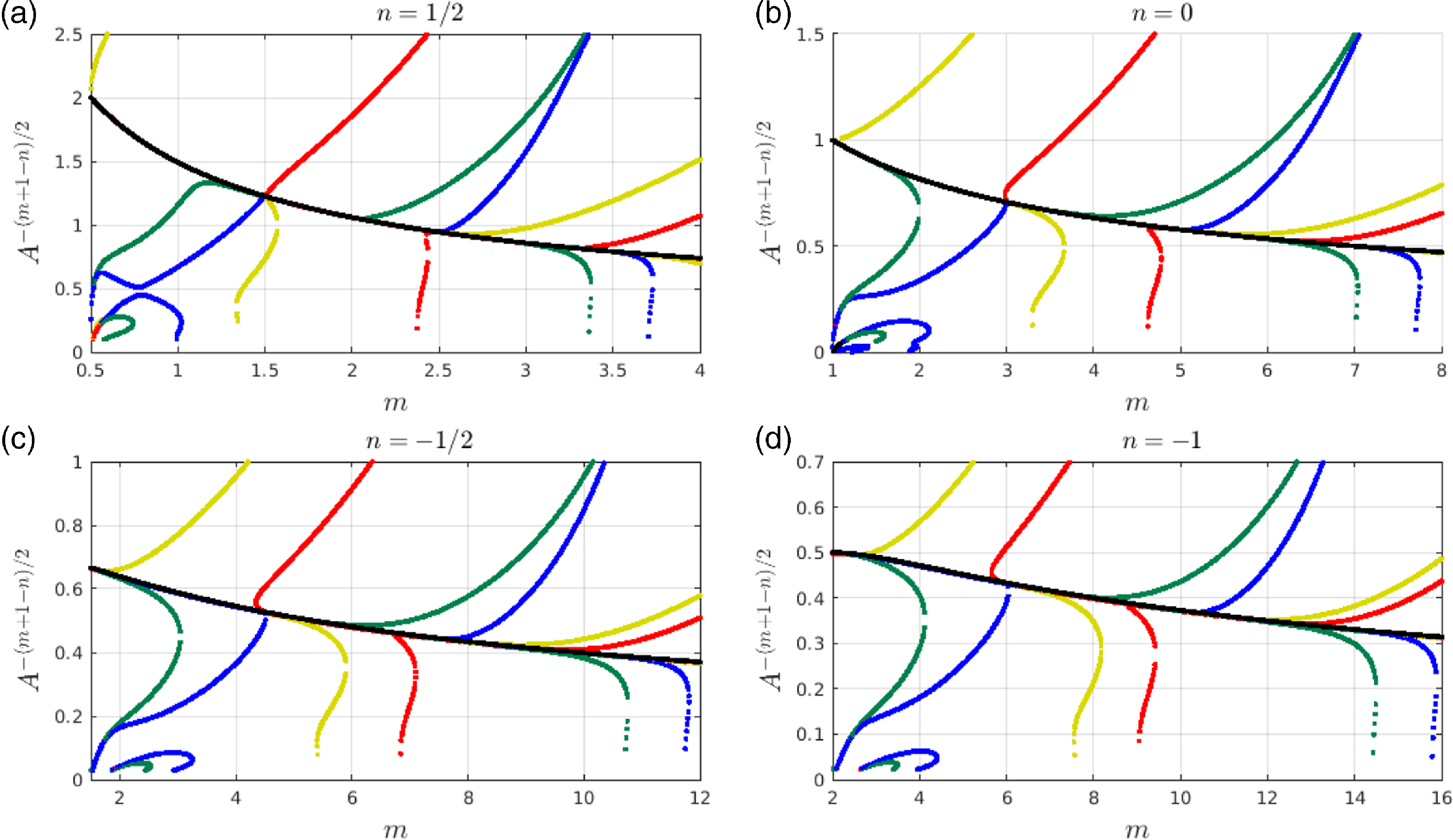
, respectively. Similar bifurcation diagrams have been presented in the authors’ previous work, [Reference Foster, Gysbers, King and Pelinovsky5, Reference Foster and Pelinovsky6], but this is the first time that solutions reaching states (c) or (d) have been found. In the former case, one viable solution with a receding interface (blue), satisfying (3.24), was identified, as well as one with an attached interface (yellow), satisfying (3.26). In the latter case, two viable solutions were found, one with the local behaviour (3.26), which is a potential profile prior to touchdown (green), and another with an advancing interface (red) and the near-field behaviour (3.23). Similar experiments were carried out for many values of
$n=0$
, respectively. Similar bifurcation diagrams have been presented in the authors’ previous work, [Reference Foster, Gysbers, King and Pelinovsky5, Reference Foster and Pelinovsky6], but this is the first time that solutions reaching states (c) or (d) have been found. In the former case, one viable solution with a receding interface (blue), satisfying (3.24), was identified, as well as one with an attached interface (yellow), satisfying (3.26). In the latter case, two viable solutions were found, one with the local behaviour (3.26), which is a potential profile prior to touchdown (green), and another with an advancing interface (red) and the near-field behaviour (3.23). Similar experiments were carried out for many values of $m \in (1,8)$
while retaining
$m \in (1,8)$
while retaining $n=0$
and the locations of the viable solutions are summarised in the top right panel of Figure 7. Further computations were carried out for other values of
$n=0$
and the locations of the viable solutions are summarised in the top right panel of Figure 7. Further computations were carried out for other values of $n$
, namely
$n$
, namely $-1,-1/2$
and
$-1,-1/2$
and $1/2$
, and similar results were found, see the other panels in Figure 7. In summary, we observe that for a particular pair of values of
$1/2$
, and similar results were found, see the other panels in Figure 7. In summary, we observe that for a particular pair of values of $m$
and
$m$
and $n$
it is possible to find connections between the far-field behaviour (3.27) and the near-field behaviours (3.23)–(3.26) for isolated values of
$n$
it is possible to find connections between the far-field behaviour (3.27) and the near-field behaviours (3.23)–(3.26) for isolated values of $A$
.
$A$
.
Results of the shooting scheme to detect viable solutions (3.21) for $m=4.5$
and
$m=4.5$
and $n=0$
. The upper panel, (a), shows the variation of
$n=0$
. The upper panel, (a), shows the variation of $f$
,
$f$
, $f^m df/d\xi$
and
$f^m df/d\xi$
and $\xi _{\text{term}}$
at the termination point (
$\xi _{\text{term}}$
at the termination point ( $\xi =\xi _{\text{term}}$
) with the shooting parameter
$\xi =\xi _{\text{term}}$
) with the shooting parameter $A_*$
. Candidate exceptional, touchdown and advancing trajectories are indicated by the black, green and red arrows, respectively. The lower panels, (b) and (c), show the candidate touchdown and attached trajectories (solid curves), respectively, along with a few trajectories ‘near’ to these candidates (dashed curves).
$A_*$
. Candidate exceptional, touchdown and advancing trajectories are indicated by the black, green and red arrows, respectively. The lower panels, (b) and (c), show the candidate touchdown and attached trajectories (solid curves), respectively, along with a few trajectories ‘near’ to these candidates (dashed curves).

Locations of viable solutions to the self-similar ODE for (3.21). The exceptional trajectory is indicated by the presence of a black dot. Advancing and receding interface solutions satisfying (3.23) and (3.24) are indicated by red and blue dots, respectively. A touchdown candidate with the near-field behaviour (3.25) is indicated by a green dot, and a leaking candidate, satisfying (3.26), is indicated by a yellow dot.
6.2. Forward self-similarity
When a backward similarity solution exists, as described in Section 6.1, it is a candidate for describing the local behaviour as the relevant type of singularity is approached. The immediate post-singularity behaviour is then expected to be a forward similarity solution of the form (1.8) with
 \begin{align} f(\xi ) \sim A \xi^{\alpha } \qquad \mbox{as} \quad \xi \rightarrow +\infty, \end{align}
where the admissible values of $A$
are determined by the pre-singularity backward solution; (6.1) is supplemented by the relevant boundary conditions at the interface. Importantly, the forward problem is not of eigenvalue type: in contrast to (1.7), an exponentially decaying correction to (6.1) is available and can be constructed by the Liouville-Green method, so the boundary value problem is correctly specified for given
$A$
are determined by the pre-singularity backward solution; (6.1) is supplemented by the relevant boundary conditions at the interface. Importantly, the forward problem is not of eigenvalue type: in contrast to (1.7), an exponentially decaying correction to (6.1) is available and can be constructed by the Liouville-Green method, so the boundary value problem is correctly specified for given $A$
, rather than the possible
$A$
, rather than the possible $A$
being determined as part of the solution (the corresponding quantity then being exponentially growing rather than decaying). It was proved in Corollary 4.2 of [Reference Foster and Pelinovsky6] that reversing and anti-reversing solutions emanating from suitable behaviour at finite
$A$
being determined as part of the solution (the corresponding quantity then being exponentially growing rather than decaying). It was proved in Corollary 4.2 of [Reference Foster and Pelinovsky6] that reversing and anti-reversing solutions emanating from suitable behaviour at finite $\xi$
all reach (6.1), for some value of the parameter
$\xi$
all reach (6.1), for some value of the parameter $A$
, when integrated in the direction of increasing
$A$
, when integrated in the direction of increasing $\xi$
. Associated numerical results are shown in Figure 8, for
$\xi$
. Associated numerical results are shown in Figure 8, for $n=0$
,
$n=0$
, $m=2,3,4$
, the ODE being solved in the direction of increasing
$m=2,3,4$
, the ODE being solved in the direction of increasing $\xi$
, the approach confirming that arbitrary
$\xi$
, the approach confirming that arbitrary $A\gt 0$
can be attained in this fashion.
$A\gt 0$
can be attained in this fashion.
The connection problem for the self-similar ODE for $t\gt 0$
; illustrating that connections can be made to arbitrary positive values of
$t\gt 0$
; illustrating that connections can be made to arbitrary positive values of $A$
(viable reversers have
$A$
(viable reversers have $A \lt A_*$
and viable anti-reversers have
$A \lt A_*$
and viable anti-reversers have $A \gt A_*$
).
$A \gt A_*$
).

7. Specific singular phenomena
7.1. Preliminaries
We shall exploit the $x$
and
$x$
and $t$
translation invariance of (1.1) to locate the singularity at
$t$
translation invariance of (1.1) to locate the singularity at $x=0$
and
$x=0$
and $t=0$
, without loss of generality (in particular, where a fixed boundary is involved, this will be taken to be at
$t=0$
, without loss of generality (in particular, where a fixed boundary is involved, this will be taken to be at $x=0$
). These symmetries will play further important roles in what follows.
$x=0$
). These symmetries will play further important roles in what follows.
Section 5 gives a detailed description of the two relevant linearisations in terms of special functions. Here we summarise the results in more informal terms and in a self-contained fashion to highlight the information we shall need in the rest of the section. Firstly, the linearisation (5.1) about the spatially uniform solution
 \begin{align} h=((1-n)({-}t))^{\frac{1}{1-n}}, \end{align}
leads to the linear PDE (5.2). The relevant backward similarity solutions to this PDE take the form
 \begin{align}{\mathcal H}_M= ({-}t)^{\frac{n}{1-n}}({-}t)^{\frac{(m+1-n)M}{2(1-n)}} \Psi _M(\eta ), \quad \eta =\sqrt{\frac{m+1-n}{2}} (1-n)^{-\frac{(m+1-n)}{2(1-n)}} \frac{x }{({-}t)^{\frac{(m+1-n)}{2(1-n)}}}, \end{align}
for non-negative integer $M$
,
$M$
, $\Psi _M$
being an
$\Psi _M$
being an $M$
th order polynomial in
$M$
th order polynomial in $\eta$
that satisfies
$\eta$
that satisfies
 \begin{align} -M \Psi _M + \eta \frac{d \Psi _M}{d \eta }=\frac{d^2 \Psi _M}{d \eta ^2}. \end{align}
We normalise $\Psi _M(\eta )$
by requiring that
$\Psi _M(\eta )$
by requiring that
 \begin{align} \Psi _M \sim \eta ^M \qquad \mbox{as} \quad |\eta | \rightarrow \infty, \end{align}
so that
 \begin{align} \Psi _0=1, \quad \Psi _1=\eta, \quad \Psi _2=\eta ^2-1, \quad \Psi _3=\eta ^3-3 \eta, \quad \Psi _4=\eta ^4-6 \eta ^2 +3. \end{align}
The coefficients in $\Psi _M$
alternate in sign, so that the constant term in
$\Psi _M$
alternate in sign, so that the constant term in $\Psi _{2N}$
has the same sign as
$\Psi _{2N}$
has the same sign as $({-}1)^N$
, as does the linear term in
$({-}1)^N$
, as does the linear term in $\Psi _{2N+1}$
, an observation that will be relevant in due course. In view of the power of
$\Psi _{2N+1}$
, an observation that will be relevant in due course. In view of the power of $({-}t)$
in the prefactor in (7.2), self-consistency, in the sense that the second term in (5.1) is much smaller than the first in the limit
$({-}t)$
in the prefactor in (7.2), self-consistency, in the sense that the second term in (5.1) is much smaller than the first in the limit $t \rightarrow 0^-$
, requires
$t \rightarrow 0^-$
, requires
 \begin{align} m M +(1-n)(M-2)\gt 0, \end{align}
which is automatically satisfied for $M \geq 1$
in the range of interest here but fails for
$M \geq 1$
in the range of interest here but fails for $M=0$
; the full complement of
$M=0$
; the full complement of $M$
is required to furnish a complete set of eigenfunctions to (5.2), an issue to which we shall also implicitly need to return.
$M$
is required to furnish a complete set of eigenfunctions to (5.2), an issue to which we shall also implicitly need to return.
Similar issues arise for the linearisation about the steady state
 \begin{align} h=A_* x^{\frac{2}{m+1-n}}, \end{align}
for which $\bar{\mathcal H}$
, the perturbation about (7.7), satisfies the linear PDE (5.10), which is more conveniently written in the form
$\bar{\mathcal H}$
, the perturbation about (7.7), satisfies the linear PDE (5.10), which is more conveniently written in the form
 \begin{align} \frac{\partial \bar{\mathcal H}}{\partial t} = A_* ^m \left (\frac{\partial ^2}{\partial x^2} \left ( x^{\frac{2m}{m+1-n}} \bar{\mathcal H} \right ) - \left (\frac{2 n (m+n+1)}{(m+1-n)^2}\right ) x^{-\frac{2(1-n)}{m+1-n}} \bar{\mathcal H} \right ). \end{align}
Since we limit ourselves to the range $m+3n+1\gt 0$
, the required backward self-similar solutions to (5.10) (i.e. those with maximal regularity as
$m+3n+1\gt 0$
, the required backward self-similar solutions to (5.10) (i.e. those with maximal regularity as $\eta \rightarrow 0^+$
, this being a requirement for the subsequent matching) take the form
$\eta \rightarrow 0^+$
, this being a requirement for the subsequent matching) take the form
 \begin{align} \bar{\mathcal H}_M= ({-}t)^{\frac{n+1-m}{2(1-n)}} ({-}t)^M \eta^{\frac{n+1-m}{m+1-n}} \Theta _M(\eta ), \qquad \eta = A_*^{-\frac{m(m+1-n)}{2(1-n)}} x ({-}t)^{-\frac{m+1-n}{2(1-n)}}, \end{align}
where $\Theta _M(\eta )$
is a polynomial in
$\Theta _M(\eta )$
is a polynomial in $\eta^{\frac{2(1-n)}{m+1-n}}$
of
$\eta^{\frac{2(1-n)}{m+1-n}}$
of $M$
th order, with
$M$
th order, with
 \begin{align} -M \Theta _M + \frac{m+1-n}{2(1-n)} \eta \frac{d \Theta _M}{d \eta }= \eta^{-\frac{n+1-m}{m+1-n}}\frac{d^2 }{d \eta ^2} \left ( \eta^{\frac{m+1+n}{m+1-n}} \Theta _M \right )- \frac{2 n (m+1+n)}{(m+1-n)^2} \eta^{-\frac{2(1-n)}{m+1-n}} \Theta _M. \end{align}
We note that $\eta$
in (7.9) has the same time dependence as in (7.2), being that of the full similarity solution of Section 6.1, though the constant factor for convenience differs. We normalise
$\eta$
in (7.9) has the same time dependence as in (7.2), being that of the full similarity solution of Section 6.1, though the constant factor for convenience differs. We normalise $\Theta _M(\eta )$
according to
$\Theta _M(\eta )$
according to
 \begin{align} \Theta _M \sim \eta^{\frac{2(1-n) M}{m+1-n}} \qquad \mbox{as} \quad \eta \rightarrow + \infty ; \end{align}
the coefficients again alternate sign, so that $\Theta _M(0)$
has the same sign as
$\Theta _M(0)$
has the same sign as $({-}1)^M$
; in contrast to
$({-}1)^M$
; in contrast to $\Psi _M$
, for which the polynomials are alternately odd and even,
$\Psi _M$
, for which the polynomials are alternately odd and even, $\Theta _M$
contains all the relevant powers. It follows that
$\Theta _M$
contains all the relevant powers. It follows that
 \begin{align} \Theta _0=1, \qquad \qquad \qquad \Theta _1=\eta^{\frac{2(1-n)}{m+1-n}}-2 \frac{(1-n)(n+m+3)}{(m+1-n)^2}, \end{align}
 \begin{align} \Theta _2=\eta^{\frac{4(1-n)}{m+1-n}}-4 \frac{(1-n)(m+5-n)}{(m+1-n)^2} \eta^{\frac{2(1-n)}{m+1-n}} +4 \frac{(1-n)^2(m+5-n)(n+m+3)}{(m+1-n)^4 }. \end{align}
Given that (7.7) is proportional to $({-}t)^{1/(1-n)}$
for
$({-}t)^{1/(1-n)}$
for $\eta =O(1)$
, self-consistency of (7.9) requires that
$\eta =O(1)$
, self-consistency of (7.9) requires that
 \begin{align} m\lt (2M-1)(1-n) \end{align}
7.2. Extinction behaviour
We start with this case because it involves only one class of self-similar solutions (these being those of the limit problem in Section 4.2, rather than those of the full PDE) and does not involve any post-singular behaviour, $h$
being identically zero following extinction; moreover, it illustrates some principles that will be of more general relevance. We refer to [Reference Grundy13] for a very closely related approach to this case.
$h$
being identically zero following extinction; moreover, it illustrates some principles that will be of more general relevance. We refer to [Reference Grundy13] for a very closely related approach to this case.
The extinction behaviour is ‘flat’ in the sense that it is selected by the linearisation (5.1), with $M$
even in (7.2); in other words, we have ‘inner’ expansion
$M$
even in (7.2); in other words, we have ‘inner’ expansion
 \begin{align} h \sim \left ((1-n) ({-}t)\right )^{\frac{1}{1-n}} - a_N ({-}t)^{\frac{n+(m+1-n)N}{1-n}} \Psi _{2N}(\eta ),, \end{align}
with $N\geq 1$
and where
$N\geq 1$
and where $a_N$
is an arbitrary constant that is required to be positive in view of the matching to
$a_N$
is an arbitrary constant that is required to be positive in view of the matching to $b_N$
noted below. In view of (7.4), the expression (7.15) disorders for
$b_N$
noted below. In view of (7.4), the expression (7.15) disorders for $|x| \geq O(({-}t)^{\frac{1}{2N}})$
(i.e. the final ‘linearised’ term in (7.15) becomes comparable with the leading
$|x| \geq O(({-}t)^{\frac{1}{2N}})$
(i.e. the final ‘linearised’ term in (7.15) becomes comparable with the leading $\left ((1-n) ({-}t)\right )^{\frac{1}{1-n}}$
term). On this outer scale, the dominant balance in (1.1) is given by
$\left ((1-n) ({-}t)\right )^{\frac{1}{1-n}}$
term). On this outer scale, the dominant balance in (1.1) is given by
 \begin{align*} \frac{\partial h}{\partial t} \sim - h^n \end{align*}
so that (cf. Section 4.2)
 \begin{align} h \sim ({-}t)^{\frac{1}{1-n}} \left ((1-n) \left (1-b_N \frac{x^{2N}}{({-}t)} \right )\right )^{\frac{1}{1-n}} \end{align}
with $b_N \propto a_N$
; the matching condition (‘inner of outer’) that follows from (7.16) can readily be inferred. From (7.16) it follows that the interfaces satisfy
$b_N \propto a_N$
; the matching condition (‘inner of outer’) that follows from (7.16) can readily be inferred. From (7.16) it follows that the interfaces satisfy
 \begin{align*} x \sim \pm \left ( \frac{({-}t)}{b_N} \right )^{\frac{1}{2N}} \qquad \mbox{as} \quad t \rightarrow 0^-, \end{align*}
wherein $b_N$
is an arbitrary positive constant.
$b_N$
is an arbitrary positive constant.
We now discuss the status of $N$
in the analysis above in terms of the stability (reflecting the completeness of the eigenfunctions) and of the necessity for an entire family of possible asymptotic behaviours (
$N$
in the analysis above in terms of the stability (reflecting the completeness of the eigenfunctions) and of the necessity for an entire family of possible asymptotic behaviours ( $N$
being an arbitrary positive integer). The case
$N$
being an arbitrary positive integer). The case $N=1$
is expected to provide the generic (i.e. stable) extinction behaviour; while the solution to (5.2) will in general also contain
$N=1$
is expected to provide the generic (i.e. stable) extinction behaviour; while the solution to (5.2) will in general also contain ${\mathcal H}_0$
and
${\mathcal H}_0$
and ${\mathcal H}_1$
contributions, each of these being eliminated by identifying
${\mathcal H}_1$
contributions, each of these being eliminated by identifying $x=0$
,
$x=0$
, $t=0$
with the place and time of extinction (it is no coincidence that there are two translation symmetries and that two eigenfunctions need to be suppressed); indeed,
$t=0$
with the place and time of extinction (it is no coincidence that there are two translation symmetries and that two eigenfunctions need to be suppressed); indeed, ${\mathcal H}_0$
corresponds to a small shift in
${\mathcal H}_0$
corresponds to a small shift in $t$
in (1.6), while
$t$
in (1.6), while ${\mathcal H}_M \propto \partial{\mathcal H}_{M+1}/\partial x$
, so an
${\mathcal H}_M \propto \partial{\mathcal H}_{M+1}/\partial x$
, so an $x$
translation in
$x$
translation in ${\mathcal H}_2$
can suppress
${\mathcal H}_2$
can suppress ${\mathcal H}_1$
. Similar arguments apply in the singular scenarios outlined below, where we typically omit such details (see the end of Section 5.2, however). The necessity for the non-generic cases
${\mathcal H}_1$
. Similar arguments apply in the singular scenarios outlined below, where we typically omit such details (see the end of Section 5.2, however). The necessity for the non-generic cases $N \geq 2$
can be argued as follows: for initial data containing a minimum between the two maxima, two generic behaviours can occur prior to extinction:
$N \geq 2$
can be argued as follows: for initial data containing a minimum between the two maxima, two generic behaviours can occur prior to extinction:
-
1. diffusion may eliminate the minimum to leave a single maximum or
-
2. the sink term may lead to the minimum touching down (as described in the next subsection), with the support of
$h$
breaking into two disconnected sets.

The case $N=2$
(which has a minimum at
$N=2$
(which has a minimum at $\eta =0$
) describes intermediate-asymptotic behaviour on the borderline between these two, with yet higher
$\eta =0$
) describes intermediate-asymptotic behaviour on the borderline between these two, with yet higher $N$
corresponding to borderlines between scenarios that are themselves non-generic (the inevitability of the latter being implicit in the above identification of the necessity of a scenario with
$N$
corresponding to borderlines between scenarios that are themselves non-generic (the inevitability of the latter being implicit in the above identification of the necessity of a scenario with $N=2$
, enabling a bootstrapping argument to higher and higher
$N=2$
, enabling a bootstrapping argument to higher and higher $N$
given the presence of the comparable families associated with other types of singular behaviour).
$N$
given the presence of the comparable families associated with other types of singular behaviour).
In summary, as well as characterising a particularly significant type of intermediate-asymptotic behaviour, the above illustrates a central element of the subsequent subsections, namely the existence of a (discrete) set of asymptotic possibilities, the leading one of which is generic, this being particularly transparent in the current case given that the relevant solution to the heat equation can be written as a sum over the Hermite polynomials (5.5) with $k \geq 2$
. The number of modes to which a given asymptotic scenario is unstable is readily identified from such a representation in terms of the omitted contributions and the non-generic behaviours play an identifiable role in the dynamics: for example, and as noted above, the case
$k \geq 2$
. The number of modes to which a given asymptotic scenario is unstable is readily identified from such a representation in terms of the omitted contributions and the non-generic behaviours play an identifiable role in the dynamics: for example, and as noted above, the case $C_2 = C_3 = 0$
can be interpreted as providing the borderline between solutions whose support breaks up prior to extinction and those for which it does not.
$C_2 = C_3 = 0$
can be interpreted as providing the borderline between solutions whose support breaks up prior to extinction and those for which it does not.
7.3. Touchdown
It is noteworthy that there are three distinct intermediate-asymptotic scenarios in this case. Firstly, the results of the previous subsection can be immediately revisited with the only changes being $a_N \rightarrow -a_{N}$
and
$a_N \rightarrow -a_{N}$
and $b_N \rightarrow -b_{N}$
, with
$b_N \rightarrow -b_{N}$
, with $a_N$
and
$a_N$
and $b_N$
then still positive. Hence, in particular, (7.16) becomes
$b_N$
then still positive. Hence, in particular, (7.16) becomes
 \begin{align} h \sim ({-}t)^{\frac{1}{1-n}} \left ( (1-n) \left ( 1 + b_N \frac{x^{2N}}{({-}t)} \right ) \right )^{\frac{1}{1-n}} \end{align}
so that the local profile at $t=0$
is given by
$t=0$
is given by
 \begin{align*} h(x,0) \sim \left ( (1-n) b_N x^{2N} \right )^{\frac{1}{1-n}} \qquad \mbox{as} \quad |x| \rightarrow 0. \end{align*}
For $t \rightarrow 0^+$
(i.e. after the touchdown and film rupture at
$t \rightarrow 0^+$
(i.e. after the touchdown and film rupture at $t=0$
), one then has the asymptotic behaviour
$t=0$
), one then has the asymptotic behaviour
 \begin{align} h \sim \left ( (1-n) \left (b_N x^{2N} -t \right ) \right )^{\frac{1}{1-n}} \end{align}
with retracting interfaces given by
 \begin{align*} x\sim \pm \left ( \frac{t}{b_N} \right )^{\frac{1}{2N}}, \end{align*}
and with $h \equiv 0$
for smaller
$h \equiv 0$
for smaller $|x|$
; since (7.18) is consistent with (2.2), the former needs no supplementation by an inner scaling.
$|x|$
; since (7.18) is consistent with (2.2), the former needs no supplementation by an inner scaling.
Secondly, the green curves in Figure 7 are of the required type for the pre-touchdown local behaviour, while the associated post-touchdown local behaviour is then expected to be a forward similarity solution of the form (1.7).
Thirdly, and clarifying the bifurcation structure in Figure 7, the black branch therein, which gives the exceptional solution, can be followed in the sense of the linearisation (5.10), so that
 \begin{align} h \sim \left \{ \begin{array}{l@{\quad}l@{\quad}l} \displaystyle A_* x^{\frac{2}{m+1-n}} + c_M^+ \bar{\mathcal H}_M(x,t) & \mbox{for} & \eta \gt 0, \\[9pt] \displaystyle A_* ({-}x)^{\frac{2}{m+1-n}} + c_M^- \bar{\mathcal H}_M({-}x,t) & \mbox{for} & \eta \lt 0, \end{array} \right. \end{align}
provides the outer (i.e. $\eta =O(1)$
) expansion, with arbitrary constants
$\eta =O(1)$
) expansion, with arbitrary constants $c_M^{\pm }$
and
$c_M^{\pm }$
and $\bar{\mathcal H}_M$
and
$\bar{\mathcal H}_M$
and $\eta$
as in (7.9). Here, the pre-touchdown solution of Section 3.1, see (3.8), comes into play via its quasi-steady generalisation: the resulting inner scalings are
$\eta$
as in (7.9). Here, the pre-touchdown solution of Section 3.1, see (3.8), comes into play via its quasi-steady generalisation: the resulting inner scalings are
 \begin{align} x=({-}t)^M \xi, \qquad h=({-}t)^{\frac{2M}{m+1-n}} g(\xi ) \end{align}
implying the quasi-steady balance (as in Section 3.1)
 \begin{align} \frac{d }{d \xi } \left ( g^m \frac{d g }{d \xi } \right ) \sim g^n \end{align}
at leading order. The matching condition
 \begin{align} g \sim A_* |\xi |^{\frac{2}{m+1-n}} \qquad \mbox{as} \quad |\xi | \rightarrow \infty \end{align}
specifies the solution to (7.21) up to arbitrary constants $\xi _0$
and
$\xi _0$
and $\alpha$
in the form
$\alpha$
in the form
 \begin{align} g=\alpha ^2 G\left ( \frac{\xi +\xi _0}{\alpha^{m+1-n}} \right ) \end{align}
where $G(\sigma )$
is an even function of
$G(\sigma )$
is an even function of $\sigma$
that can be specified uniquely via
$\sigma$
that can be specified uniquely via
 \begin{align} & G(\sigma ) \sim A_* \sigma^{\frac{2}{m+1-n}} +\sigma^{\frac{n+1-m}{m+1-n}} \qquad \mbox{as} \quad \sigma \rightarrow +\infty \qquad \mbox{for} \quad n \gt 0, \nonumber \\[5pt] & G(\sigma ) \sim A_* \sigma^{\frac{2}{m+1-n}} -\sigma^{\frac{n+1-m}{m+1-n}} \qquad \mbox{as} \quad \sigma \rightarrow +\infty \qquad \mbox{for} \quad n \lt 0,\end{align}
The switch in sign follows (as in (3.10) above) from an analysis of the integral that arises on solving the separable equation
 \begin{align*} \frac{1}{2} G^{2m} \left ( \frac{d G }{d \sigma } \right )^2 -\frac{1}{m+n+1} \left ( G^{m+n+1} -G_0^{m+n+1} \right )=0 \end{align*}
that results as the first integral of (7.21), where
 \begin{align*} G_0=G(0). \end{align*}
In the special case $n=0$
already noted above, we have
$n=0$
already noted above, we have
 \begin{align*} G=\left ( G_0 + \frac{m+1}{2} \sigma ^2 \right )^{\frac{1}{m+1}} \end{align*}
and the correction terms in (7.24) are instead absent; we omit further analysis of this exceptional case here.
Given that
 \begin{align} \bar{\mathcal H}_M \sim K_M ({-}1)^M ({-}t)^M x^{\frac{n+1-m}{m+1-n}} \qquad \mbox{as} \quad \eta \rightarrow 0. \end{align}
for some positive constant $K_M$
that is to be regarded as known, given the analysis of Section 5.2, matching to (7.20) and (7.24) implies that
$K_M$
that is to be regarded as known, given the analysis of Section 5.2, matching to (7.20) and (7.24) implies that $\alpha$
and
$\alpha$
and $\xi _0$
are given by
$\xi _0$
are given by
 \begin{align} & \frac{2}{m+1-n} \xi _0 A_* \pm \alpha^{m+1-n} = ({-}1)^M c_M^+ K_M \nonumber\\[5pt]& -\frac{2}{m+1-n} \xi _0 A_* \pm \alpha^{m+1-n} = ({-}1)^M c_M^- K_M \end{align}
where the signs on the left-hand sides correspond to those in (7.24). Self-consistency of such a scenario requires that (7.14) hold. Before turning to questions of stability, it is helpful to make connections between (7.26) and Figure 7; the green branches in the latter bifurcate off when equality holds in (7.14) and are symmetric. For $m$
slightly larger than
$m$
slightly larger than $(2M-1)(1-n)$
, the expressions (7.26) remain relevant with
$(2M-1)(1-n)$
, the expressions (7.26) remain relevant with $\xi _0=0$
,
$\xi _0=0$
, $c_M^+=c_M^-=c_M$
; since
$c_M^+=c_M^-=c_M$
; since $\alpha$
is necessarily positive (a constraint with broader implications in (7.26)), this implies
$\alpha$
is necessarily positive (a constraint with broader implications in (7.26)), this implies $c_M\gt 0$
and hence
$c_M\gt 0$
and hence $A\gt A_*$
for
$A\gt A_*$
for $n\lt 0$
,
$n\lt 0$
, $M$
odd and
$M$
odd and $n\gt 0$
,
$n\gt 0$
, $M$
even, with
$M$
even, with $c_M\lt 0$
and
$c_M\lt 0$
and $A\lt A_*$
in the converse cases. This is consistent both with the alternating directions of the green branches in Figure 7 and with their swapping sides as
$A\lt A_*$
in the converse cases. This is consistent both with the alternating directions of the green branches in Figure 7 and with their swapping sides as $n$
passes through zero. Turning now to stability,
$n$
passes through zero. Turning now to stability, $N=1$
in (7.17) leads to a generic cases, as in the previous subsection;
$N=1$
in (7.17) leads to a generic cases, as in the previous subsection; $N \geq 2$
scenarios are again necessary but unstable. We signpost that the cases akin to (7.17), but with
$N \geq 2$
scenarios are again necessary but unstable. We signpost that the cases akin to (7.17), but with $M$
odd, will also be relevant in due course. In terms of (7.19), the cases
$M$
odd, will also be relevant in due course. In terms of (7.19), the cases $\eta \gt 0$
and
$\eta \gt 0$
and $\eta \lt 0$
in effect operate independently, so suppressing the
$\eta \lt 0$
in effect operate independently, so suppressing the $M=0$
mode in (5.10) on both sides uses up both translational invariants. Since (7.14) is violated for
$M=0$
mode in (5.10) on both sides uses up both translational invariants. Since (7.14) is violated for $M=1$
,
$M=1$
, $m+n\gt 1$
, the first legitimate instance of (7.19) is doubly unstable (though in the symmetric case, or with zero-Neumann boundary condition on
$m+n\gt 1$
, the first legitimate instance of (7.19) is doubly unstable (though in the symmetric case, or with zero-Neumann boundary condition on $x=0$
(for which
$x=0$
(for which $x$
translational invariance cannot be exploited), it is only singly so). However, for related reasons the left-most green branch in panel of Figure 7 with
$x$
translational invariance cannot be exploited), it is only singly so). However, for related reasons the left-most green branch in panel of Figure 7 with $n \leq 0$
is expected to be stableFootnote 4 above the fold, but unstable below it: in these regimes there are thus two stable scenarios, that in Figure 7 for a narrow range of
$n \leq 0$
is expected to be stableFootnote 4 above the fold, but unstable below it: in these regimes there are thus two stable scenarios, that in Figure 7 for a narrow range of $m\gt 1-n$
, while (7.17) with
$m\gt 1-n$
, while (7.17) with $N=1$
is applicable throughout. In Figure 7, successive branches (of any colour) are expected to gain an additional unstable mode on each occasion a bifurcation point is passed through from left to right.
$N=1$
is applicable throughout. In Figure 7, successive branches (of any colour) are expected to gain an additional unstable mode on each occasion a bifurcation point is passed through from left to right.
At $t=0$
, the spatial profiles in the third scenario take the form
$t=0$
, the spatial profiles in the third scenario take the form
 \begin{align} h \sim A_* |x|^{\frac{2}{m+1-n} } + c_M^{\pm } |x|^{\frac{n+1-m+2M(1-n)}{m+1-n} } \qquad \mbox{as} \quad |x| \rightarrow 0. \end{align}
There seems subsequently to be the possibility of non-uniqueness, but we shall not discuss the associated post-touchdown behaviour given that these are in any case unstable.
7.4. Attachment, detachment and coalescence
Attachment, either to a fixed boundary or through two interfaces colliding (either through both advancing or by one advancing faster than the other is retracting) – termed coalescence above – raises no pre-singularity questions since the solution has no prior knowledge that it is about to attach (unlike the other cases analysed here).Footnote 5 Post-attachment raises no significant challenges either: one has a porous-medium equation similarity solution of the form
 \begin{align*} h \sim t^{\frac{1}{m}} f \left ( \frac{x}{t} \right ) \qquad \mbox{as} \quad \mbox{with} \quad x=O(t), \end{align*}
with additional structure when an advancing interface overuns a receding one of a form akin to that analysed in the generic anti-reverser case addressed below. One related observation is in order; however, the pre-attaching behaviour of an advancing interface takes the form
 \begin{align*} h \sim ({-}t)^{\frac{1}{m}} f \left ( \frac{x}{({-}t)} \right ), \qquad f^m(\eta )=m\eta _0(\eta _0-\eta ) \end{align*}
for some constant $\eta _0$
. This simply corresponds to a Taylor expansion in
$\eta _0$
. This simply corresponds to a Taylor expansion in $t$
of (2.3), reflecting the lack of prior knowledge referred to above, but is also an exceptional connection for the porous-medium equation in a sense elaborated upon in [Reference Hulshof, King and Bowen14], the significance of which here is that this relates to the probably unexpected branches present in the bottom left-hand corners of Figure 7, though we shall not go into details here.
$t$
of (2.3), reflecting the lack of prior knowledge referred to above, but is also an exceptional connection for the porous-medium equation in a sense elaborated upon in [Reference Hulshof, King and Bowen14], the significance of which here is that this relates to the probably unexpected branches present in the bottom left-hand corners of Figure 7, though we shall not go into details here.
There are of course non-generic attaching behaviours, such as an interface reversing at the same instant as attaching, but the no-prior-knowledge argument applies to these also. For the hole filling case in higher dimensions, the situation is more complicated, however, since the interface is aware of its increasing curvature; see, for example, [Reference Angenent, Aronson, Betelu and Lowengrub1] for the porous-medium equation – including a sink term, as in (1.1), leads to open questions in this regard.
The detachment case is also simple in the sense that we conjecture that the left-most yellow branch in each panel of Figure 7 provides the generic behaviour, with post-detachment being described by an associated forward similarity solution. For $n\gt 0$
, we expect this branch to start from
$n\gt 0$
, we expect this branch to start from $A\lt A_*$
as
$A\lt A_*$
as $m+n \rightarrow 1^+$
(with a fold in
$m+n \rightarrow 1^+$
(with a fold in $m+n\lt 1$
connecting the branch to
$m+n\lt 1$
connecting the branch to $A=A_*$
at
$A=A_*$
at $m+n=1$
), whereas for
$m+n=1$
), whereas for $n\leq 0$
we have
$n\leq 0$
we have $A \rightarrow A_*$
in that limit. Non-generic cases arise both as the other yellow branches and from tracking along the black branch prior to the secondary and subsequent bifurcations, as in the first of (7.19), being subject to (7.14). Now a quasi-steady version of the leaking solution of Section 3.1, satisfying (3.6), describes the inner behaviour – the inner scalings are again given by (7.20), but now (7.21) is subject to
$A \rightarrow A_*$
in that limit. Non-generic cases arise both as the other yellow branches and from tracking along the black branch prior to the secondary and subsequent bifurcations, as in the first of (7.19), being subject to (7.14). Now a quasi-steady version of the leaking solution of Section 3.1, satisfying (3.6), describes the inner behaviour – the inner scalings are again given by (7.20), but now (7.21) is subject to
 \begin{align*} g=0 \qquad \mbox{at} \quad \xi =0 \end{align*}
so that
 \begin{align*} g=\alpha ^2 G \left ( \frac{\xi }{\alpha^{m+n-1}} \right ) \end{align*}
with
 \begin{align*} \frac{1}{2} G^{2m} \left ( \frac{d G}{d \sigma } \right )^2 -\frac{1}{m+1} G^{m+n+1} =\frac{1}{2} J_0^2 \end{align*}
where
 \begin{align*} J_0=G^m \left. \frac{d G}{d \sigma } \right |_{\sigma =0} \gt 0 \end{align*}
determines the outward flux. For $n=0$
, we have
$n=0$
, we have
 \begin{align*} G=\left ( (m+1) \left (J_0 \sigma + \frac{1}{2} \sigma ^2 \right )\right )^{\frac{1}{m+1}} \end{align*}
and for any $n$
the sign in the first of (7.24) applies here – correspondingly, the yellow branches of Figure 7 are on the opposite sides from the green ones for
$n$
the sign in the first of (7.24) applies here – correspondingly, the yellow branches of Figure 7 are on the opposite sides from the green ones for $n\lt 0$
and on the same side for
$n\lt 0$
and on the same side for $N\gt 0$
. The local behaviour at detachment is then again as in (7.27). Instability follows even for
$N\gt 0$
. The local behaviour at detachment is then again as in (7.27). Instability follows even for $M=2$
because the
$M=2$
because the $x$
-translation mode is not available given the boundary condition (i.e.
$x$
-translation mode is not available given the boundary condition (i.e. $h=0$
at
$h=0$
at $x=0$
), and the
$x=0$
), and the $M=0$
and
$M=0$
and $M=1$
modes both need to be absent; accordingly, we omit any discussion of the post-detachment behaviour in these non-generic cases.
$M=1$
modes both need to be absent; accordingly, we omit any discussion of the post-detachment behaviour in these non-generic cases.
7.5. Reversers and anti-reversers
We start with scenarios in which the two have closely related behaviour, before discussing a (generic) anti-reversing structure distinct from the other categories arising here. We take the support to lie in $x\gt 0$
at
$x\gt 0$
at $t=0$
and start from the first of (7.19) (writing
$t=0$
and start from the first of (7.19) (writing $c_M=c_M^+$
) with, as always, (7.14) being required. Since here we can apply both
$c_M=c_M^+$
) with, as always, (7.14) being required. Since here we can apply both $t$
and
$t$
and $x$
translational invariance, the
$x$
translational invariance, the $M=0$
and
$M=0$
and $M=1$
modes can both be suppressed (in contrast to the situation in the previous section), leaving
$M=1$
modes can both be suppressed (in contrast to the situation in the previous section), leaving $M=2$
as a potential stable scenario for
$M=2$
as a potential stable scenario for $m\lt 3(1-n)$
. The matching condition
$m\lt 3(1-n)$
. The matching condition
 \begin{align} h \sim A_* x^{\frac{2}{m+1-n}} + ({-}1)^M K_M c_M ({-}t)^M x^{\frac{n+1-m}{m+1-n}} \end{align}
then applies on a travelling-wave inner region, for which a translation
 \begin{align} x=s(t)+z, \qquad s(t) \sim \frac{({-}1)^{M+1} K_M c_M}{A_*} ({-}t)^M \end{align}
is required, with the dominant balance being (as in Section 3.2)
 \begin{align} -\dot{s} \frac{\partial h}{\partial z} \sim \frac{\partial }{\partial z} \left ( h^m \frac{\partial h}{\partial z} \right ) -h^n, \end{align}
which implies that the inner scalings are
 \begin{align} z=O \left ( ({-}t)^{\frac{(m+1-n)(M+1)}{m+n-1}} \right ), \qquad h=O \left ( ({-}t)^{\frac{2(M-1)}{m+n-1}} \right ). \end{align}
Given that the outer scaling associated with (7.19) is the full self-similar one, $x=O \left ( ({-}t)^{\frac{m+1-n}{2(1-n)}} \right )$
, consistency conditions on the above read
$x=O \left ( ({-}t)^{\frac{m+1-n}{2(1-n)}} \right )$
, consistency conditions on the above read
 \begin{align} \frac{(m+1-n)(M-1)}{m+n-1} \gt M \gt \frac{m+1-n}{2(1-n)}, \end{align}
both inequalities simply reproducing (7.14). Whether (7.28) is associated with a reverser or an anti-reverser depends upon the sign of $c_M$
; if
$c_M$
; if $c_M ({-}1)^{M+1}$
is positive the above asymptotic behaviour corresponds to a reverser (advancing interface for
$c_M ({-}1)^{M+1}$
is positive the above asymptotic behaviour corresponds to a reverser (advancing interface for $t\lt 0$
), while if it is negative it is an anti-reverser (receding interface for
$t\lt 0$
), while if it is negative it is an anti-reverser (receding interface for $t\lt 0$
),Footnote 6 subject to the following qualification – for the stable case
$t\lt 0$
),Footnote 6 subject to the following qualification – for the stable case $M=2$
and other even
$M=2$
and other even $M$
the interface indeed changes direction (see (7.29)), while for
$M$
the interface indeed changes direction (see (7.29)), while for $M$
odd it recommences its original direction after an instantaneous pause (the singly unstable case
$M$
odd it recommences its original direction after an instantaneous pause (the singly unstable case $M=3$
corresponding to the borderline between (i) reversers and anti-reversers occurring in rapid succession (in either order) and (ii) no change of direction).
$M=3$
corresponding to the borderline between (i) reversers and anti-reversers occurring in rapid succession (in either order) and (ii) no change of direction).
A first integral of (7.30) is available in the case $n=0$
, namely
$n=0$
, namely
 \begin{align*} -\dot{s} h = h^m \frac{\partial h}{\partial z} -z. \end{align*}
With regard to the transcritical red/blue bifurcations in Figure 7, for $n\lt 0$
the numerics provide evidence that the primary such bifurcation has red unstable and blue stable close to the bifurcation point, though with folds rapidly swapping the stability of each, whereas for
$n\lt 0$
the numerics provide evidence that the primary such bifurcation has red unstable and blue stable close to the bifurcation point, though with folds rapidly swapping the stability of each, whereas for $n\gt 0$
the red branch is expected to be stable throughout and the blue unstable (except perhaps in the lower left-hand corner: we leave the stability of the branches there as an open question). Similar comments apply with respect to the number of unstable model arising from the subsequent bifurcations.
$n\gt 0$
the red branch is expected to be stable throughout and the blue unstable (except perhaps in the lower left-hand corner: we leave the stability of the branches there as an open question). Similar comments apply with respect to the number of unstable model arising from the subsequent bifurcations.
Collecting together the implications of the above for the generic cases, we summarise our conjectures as follows.
(I) Reversers
For $m\lt 3(1-n)$
, (7.28)–(7.30) with
$m\lt 3(1-n)$
, (7.28)–(7.30) with $M=2$
provide a stable solution, changing direction smoothly (i.e.
$M=2$
provide a stable solution, changing direction smoothly (i.e. $s \propto ({-}t)^2$
in (7.29)). At
$s \propto ({-}t)^2$
in (7.29)). At $t=0$
$t=0$
 \begin{align} h \sim A_* x^{\frac{2}{m+1-n}} + \kappa x^{\frac{5-3n-m}{m+1-n}} \end{align}
holds for some constant $\kappa$
and the
$\kappa$
and the $t \rightarrow 0^+$
behaviour follows directly from the
$t \rightarrow 0^+$
behaviour follows directly from the $t \rightarrow 0^-$
behaviour (the equivalent polynomial solutions provide the correction term, though their coefficients then all take the same sign). For
$t \rightarrow 0^-$
behaviour (the equivalent polynomial solutions provide the correction term, though their coefficients then all take the same sign). For $n\gt 0$
, the generic behaviour in
$n\gt 0$
, the generic behaviour in $m\gt 3(1-n)$
is a full similarity solution, corresponding to the first red branch in Figure 7. For
$m\gt 3(1-n)$
is a full similarity solution, corresponding to the first red branch in Figure 7. For $n\lt 0$
, the situation is slightly more complicated, with a bistable regime being present over a small range of
$n\lt 0$
, the situation is slightly more complicated, with a bistable regime being present over a small range of $m$
in
$m$
in $m\lt 3(1-n)$
, the red branch being unstable below the fold (being the borderline between the two stable scenarios) but stable above it and continuing into the range
$m\lt 3(1-n)$
, the red branch being unstable below the fold (being the borderline between the two stable scenarios) but stable above it and continuing into the range $m\gt 3(1-n)$
. When a full similarity solution applies,
$m\gt 3(1-n)$
. When a full similarity solution applies, $s$
is in general not smooth:
$s$
is in general not smooth:
 \begin{align} s \sim S_- ({-}t)^{\frac{m+1-n}{2(1-n)}} \quad \mbox{as} \quad t \rightarrow 0^-, \qquad s \sim S_+ t^{\frac{m+1-n}{2(1-n)}} \quad \mbox{as} \quad t \rightarrow 0^+, \end{align}
with a forward similarity solution holding as $t \rightarrow 0^+$
and with the constants
$t \rightarrow 0^+$
and with the constants $S_-$
and
$S_-$
and $S_+$
presumably being different and positive on the primary branch.
$S_+$
presumably being different and positive on the primary branch.
(II) Anti-reversers
The description in (I) above again applies for $m\lt 3(1-n)$
,
$m\lt 3(1-n)$
, $M=2$
(whether a reverser or anti-reverser pertains depends on the sign of
$M=2$
(whether a reverser or anti-reverser pertains depends on the sign of $\kappa$
). For
$\kappa$
). For $n\lt 0$
there is expected to be a narrow range of bistability in
$n\lt 0$
there is expected to be a narrow range of bistability in $m\gt 3(1-n)$
also (one of the stable scenarios being the full similarity solution, as in Figure 7, the other being described next), but the first blue branch is otherwise unstable, necessitating the identification of a different class of intermediate-asymptotic behaviour. The range
$m\gt 3(1-n)$
also (one of the stable scenarios being the full similarity solution, as in Figure 7, the other being described next), but the first blue branch is otherwise unstable, necessitating the identification of a different class of intermediate-asymptotic behaviour. The range $m\lt 3(1-n)$
is thus bistable, with the blue branch expected to provide the borderline between the two generic cases.
$m\lt 3(1-n)$
is thus bistable, with the blue branch expected to provide the borderline between the two generic cases.
An important clue into the other generic scenario is provided by a comparison between (2.2) and (2.3): since
 \begin{align*} 1-n\lt m \quad \mbox{for} \quad m+n\gt 1, \end{align*}
retreating interfaces are associated with local behaviour smaller than that of the advancing ones, so we may anticipate that the latter can overrun the former with little modification to itself. We now formalise that intuition; related analyses of the porous-medium equation, [Reference King and Please19, Reference Lacey20], represent precedents. Two outer regions are present on the scaling $x=O({-}t)$
, namely
$x=O({-}t)$
, namely
 \begin{align} \begin{array}{lll} \displaystyle h^m \sim m q (x-q({-}t)) &\mbox{for} & \displaystyle \frac{x}{({-}t)} \gt q,\\ \displaystyle h^{1-n} \sim (1-n) \left ({-}t+\frac{x}{Q} \right ) &\mbox{for} & \displaystyle q\gt \frac{x}{({-}t)} \gt -Q, \end{array} \end{align}
wherein $q$
and
$q$
and $Q$
are each positive constants, the former expression being a similarity solution of the porous-medium equation (as in Section 4.1) and the latter being one of the pure absorption limit (as in Section 4.2). The two expressions in (7.35) are comparable for
$Q$
are each positive constants, the former expression being a similarity solution of the porous-medium equation (as in Section 4.1) and the latter being one of the pure absorption limit (as in Section 4.2). The two expressions in (7.35) are comparable for
 \begin{align*} x=q({-}t)+ O\left ( ({-}t)^{\frac{m}{1-n}} \right ), \end{align*}
self-consistency here again requiring that $m+n\gt 1$
, which implies the inner scalings
$m+n\gt 1$
, which implies the inner scalings
 \begin{align*} x=q({-}t) + ({-}t)^{\frac{m}{1-n}} \xi, \qquad h=({-}t)^{\frac{1}{1-n}} g, \end{align*}
leading to
 \begin{align*} q \frac{\partial g}{\partial \xi } \sim \frac{\partial }{\partial \xi } \left ( g^m \frac{\partial g}{\partial \xi } \right ) \end{align*}
and hence to
 \begin{align*} q \left ( g- \left ( (1-n) \left ( 1+ \frac{q}{Q} \right )\right )^{\frac{1}{1-n}}\right ) \sim g^m \frac{\partial g}{\partial \xi }, \end{align*}
thereby matching with (7.35) in both limits $|\xi | \rightarrow \infty$
. In consequence, we simply have
$|\xi | \rightarrow \infty$
. In consequence, we simply have
 \begin{align*} h(x,0) \sim ( m q x)^{\frac{1}{m}} \qquad \mbox{as} \quad x \rightarrow 0^+ \end{align*}
so the interface obeys
 \begin{align} x \sim Q t \qquad \mbox{as} \quad t \rightarrow 0^-, \qquad x\sim -q t \qquad \mbox{as} \quad t \rightarrow 0^+, \end{align}
its velocity being discontinuous (indeed swapping sign) at $t=0$
.
$t=0$
.
There is one final, but unstable, case to which we have already alluded and for which relevant results can be read off directly from (7.17) on replacing the even exponent by an odd one, so that
 \begin{align*} h \sim ({-}t)^{\frac{1}{1-n}} \left ( (1-n) \left ( 1+b_N \frac{x^{2N+1}}{({-}t)} \right ) \right )^{\frac{1}{1-n}} \end{align*}
with $N \geq 1$
and with
$N \geq 1$
and with $b_N\gt 0$
without loss of generality. This has a retreating interface for
$b_N\gt 0$
without loss of generality. This has a retreating interface for $t\lt 0$
at
$t\lt 0$
at
 \begin{align*} x\sim -\left ( \frac{({-}t)}{b_N} \right )^{\frac{1}{2N+1}}, \end{align*}
with $h \equiv 0$
for smaller
$h \equiv 0$
for smaller $x$
, and
$x$
, and
 \begin{align*} h(x,0) \sim \left ( (1-n) b_N x^{2N+1} \right )^{\frac{1}{1-n}} \qquad \mbox{as} \quad x \rightarrow 0^+. \end{align*}
Since the interface has
 \begin{align*} x \sim \left ( \frac{t}{b_N} \right )^{\frac{1}{2N+1}} \qquad \mbox{as} \quad t \rightarrow 0^+ \end{align*}
in this case, no change of direction occurs, with $N =1$
being singly unstable and providing the borderline between solutions that lose a local maximum/minimum pair while retreating and those which touchdown. These cases are striking in having unbounded, rather than zero, interface velocity at
$N =1$
being singly unstable and providing the borderline between solutions that lose a local maximum/minimum pair while retreating and those which touchdown. These cases are striking in having unbounded, rather than zero, interface velocity at $t=0$
and do not fall naturally under any of the headings above.
$t=0$
and do not fall naturally under any of the headings above.
8. Numerical solutions to the PDE
8.1. Validation of the asymptotic predictions
Here we provide evidence to substantiate the observability of some of the local descriptions identified as generic above. First, we summarise the findings of the numerical experiments, and then, we give the details on how solutions to (1.1) were found by direct numerical simulation. All results in this section have $n=0$
but similarly good agreement is expected for other values of
$n=0$
but similarly good agreement is expected for other values of $n$
in the range (1.2).
$n$
in the range (1.2).
(i) Reversing events
Panel (ia) in Figure 9 indicates that for $m\lt 3(1-n)$
we have
$m\lt 3(1-n)$
we have $s \sim \text{const.} ({-}t)^2$
as
$s \sim \text{const.} ({-}t)^2$
as $t \to 0^-$
with the constant dependent upon the initial conditions. This is in agreement with (7.33). Panel (ib) indicates that for
$t \to 0^-$
with the constant dependent upon the initial conditions. This is in agreement with (7.33). Panel (ib) indicates that for $m\gt 3(1-n)$
we have
$m\gt 3(1-n)$
we have $s \sim \hat{\xi } ({-}t)^{(m+1-n)/2(1-n)}$
where the constant
$s \sim \hat{\xi } ({-}t)^{(m+1-n)/2(1-n)}$
where the constant $\hat{\xi }$
is that obtained from the ODE solutions described in Section 6 on the stable red branch: we find
$\hat{\xi }$
is that obtained from the ODE solutions described in Section 6 on the stable red branch: we find
 \begin{align} \hat{\xi } \approx 0.3864 \quad \mbox{for} \quad m=4, \quad n=0, \end{align}
 \begin{align} \hat{\xi } \approx 0.5014 \quad \mbox{for} \quad m=5, \quad n=0, \end{align}
the PDE simulations being consistent with these values up to three significant figures.
Comparison between the asymptotic results, shown in grey, and direct numerical simulation of (1.1), shown in black, for $n=0$
. Panels (ia) and (ib) show the interface position leading up to a reversing event for different choices of initial condition. In (ia) dashed curves are for
$n=0$
. Panels (ia) and (ib) show the interface position leading up to a reversing event for different choices of initial condition. In (ia) dashed curves are for $m=2$
, whereas solid ones are
$m=2$
, whereas solid ones are $m=3$
. In (ib), dotted curves are for
$m=3$
. In (ib), dotted curves are for $m=4$
and solid curves for
$m=4$
and solid curves for $m=5$
. Panels (ii) and (iii) show the interface position leading up to anti-reversing and attachment events, respectively, for different choices of initial condition. In both panels (ii) and (iii), dashed curves indicate
$m=5$
. Panels (ii) and (iii) show the interface position leading up to anti-reversing and attachment events, respectively, for different choices of initial condition. In both panels (ii) and (iii), dashed curves indicate $m=2$
, solid curves
$m=2$
, solid curves $m=3$
and dotted curves
$m=3$
and dotted curves $m=4$
.
$m=4$
.

(ii) Anti-reversing events
Panel (ii) in Figure 9 indicates that the interface obeys $s \sim \text{const.} ({-}t)$
with the constant selected by the initial data, in agreement with (7.36). We omit here the other regime of stable anti-reversing identified in Section 7.5, namely pure self-similarity.
$s \sim \text{const.} ({-}t)$
with the constant selected by the initial data, in agreement with (7.36). We omit here the other regime of stable anti-reversing identified in Section 7.5, namely pure self-similarity.
(iii) Attaching events
Panel (iii) in Figure 9 indicates that the interface obeys $s \sim \text{const.} ({-}t)$
with the constant selected by the initial data in agreement with the discussion in Section 7.4; in short, this is expected because the interface has no way to anticipate its collision with the absorbing boundary.
$s \sim \text{const.} ({-}t)$
with the constant selected by the initial data in agreement with the discussion in Section 7.4; in short, this is expected because the interface has no way to anticipate its collision with the absorbing boundary.
(iv) Detaching events
Panel (iv) in Figure 10 indicates that the outward flux at the interface leading up to a detachment event obeys
 \begin{align} \left. h^m \frac{\partial h}{\partial x} \right |_{x=0} = ({-}t)^{(m+1)/2} \left. f^m \frac{\partial f}{\partial \xi } \right |_{\xi =0} \end{align}
where the quantity $\left. f^m{\partial f}/{\partial \xi } \right |_{\xi =0}$
can be determined via the shooting method described in Section 6. Shooting on the self-similar ODE yields
$\left. f^m{\partial f}/{\partial \xi } \right |_{\xi =0}$
can be determined via the shooting method described in Section 6. Shooting on the self-similar ODE yields
 \begin{align} \left. f^m \frac{\partial f}{\partial \xi } \right |_{\xi =0} = 0.4912 \quad \mbox{for} \quad m=2, \quad n=0, \end{align}
 \begin{align} \left. f^m \frac{\partial f}{\partial \xi } \right |_{\xi =0} = 0.8786 \quad \mbox{for} \quad m=3, \quad n=0, \end{align}
 \begin{align} \left. f^m \frac{\partial f}{\partial \xi } \right |_{\xi =0} = 1.3076 \quad \mbox{for} \quad m=4, \quad n=0, \end{align}
with which the PDE solutions are again consistent up to three significant figures. This verifies the claim in Section 7.4 that the left-most yellow branch in Figure 7 provides the generic description of detachment.
Comparison between the asymptotic results, shown in grey, and direct numerical simulation of (1.1), shown in black, for $n=0$
; results for
$n=0$
; results for $m=2$
are indicated by dashed curves, for
$m=2$
are indicated by dashed curves, for $m=3$
with solid curves and for
$m=3$
with solid curves and for $m=4$
with dotted curves. Panel (iv) shows the flux at the interface leading up to a detachment event for different choices of initial condition. Panels (va) and (vb) show
$m=4$
with dotted curves. Panel (iv) shows the flux at the interface leading up to a detachment event for different choices of initial condition. Panels (va) and (vb) show $h$
and
$h$
and $h_{xx}$
at the minimum leading up to a touchdown event.
$h_{xx}$
at the minimum leading up to a touchdown event.

(v) Touchdown events
Panels (va) and (vb) in Figure 10 indicate that the description leading up to a touchdown event are in agreement with (7.18) with $N=1$
, verifying that this is the generic behaviour; we note that the curvature does not tend to a constant at
$N=1$
, verifying that this is the generic behaviour; we note that the curvature does not tend to a constant at $t \to 0^-$
in cases where
$t \to 0^-$
in cases where $N\gt 1$
.
$N\gt 1$
.

8.2. Numerical methods
We furnish numerical solutions (1.1) on a finite domain by supplementing it with an interface condition at the left-hand end of its compact support, that is, one of the conditions (1.3)–(1.5), as well as a symmetry condition at some location $x=x_0\gt 0$
, that is,
$x=x_0\gt 0$
, that is,
 \begin{align} \left. \frac{\partial h}{\partial x} \right |_{x=x_0} =0. \end{align}
The value of $x_0$
is chosen arbitrarily; the spatial coordinates are translated post hoc such that the singular event occurs at
$x_0$
is chosen arbitrarily; the spatial coordinates are translated post hoc such that the singular event occurs at $x=0$
.
$x=0$
.
Numerical solution is made awkward by two features, namely (a) that the domain is dynamic and (b) that the solution often exhibits an infinite spatial gradient at the interface. We alleviate these difficulties by transforming the spatial coordinates using a similar strategy to that in [Reference Foster and Pelinovsky6]. As we have seen, the solution local to an interface takes the form
 \begin{align} h \sim \lambda (t) (x-s(t))^{\omega } \quad \mbox{as} \quad x \to s(t)^+ \end{align}
for some $\lambda$
, where
$\lambda$
, where $\omega =1/m,1/(1-n),1/(m+1)$
or
$\omega =1/m,1/(1-n),1/(m+1)$
or $2/(m+1-n)$
depending on whether the interface is advancing, receding, in contact with an absorbing boundary or stationary and mass preserving. These local behaviours motivate the coordinate transformations
$2/(m+1-n)$
depending on whether the interface is advancing, receding, in contact with an absorbing boundary or stationary and mass preserving. These local behaviours motivate the coordinate transformations
 \begin{align} y = \left ( 1-\frac{x_0 - x}{x_0 - s(t)} \right )^\omega \end{align}
such that the behaviour (8.8) is replaced with $h \sim \hat{\lambda }(t) y$
as
$h \sim \hat{\lambda }(t) y$
as $y \to 0^+$
. The PDE (1.1) becomes
$y \to 0^+$
. The PDE (1.1) becomes
 \begin{align} \frac{\partial h}{\partial t} = \frac{wy^{(w-1)/w}}{x_0-s} \frac{\partial }{\partial y} \left ( \frac{wy^{(w-1)/w}}{x_0-s} h^m \frac{\partial h}{\partial y} \right ) + \frac{w \left (1-y^{1/w}\right ) y^{(w-1)/w}}{x_0 -s} \frac{ds}{dt} \frac{\partial h}{\partial y} - h^n. \end{align}
This is closed by the boundary conditions
 \begin{align} h |_{y=0} =0, \quad \left. \frac{\partial h}{\partial y}\right |_{y=1} =0, \end{align}
where the latter results from transforming (8.7) and the former results from (1.3a) for a mobile interface or (1.5) for an absorbing boundary. When an absorbing boundary is being considered we have $\dot{s}=0$
, but for a dynamic interface the motion is solved for as part of the solution to the problem using the transformed counterpart of (1.4), which reads
$\dot{s}=0$
, but for a dynamic interface the motion is solved for as part of the solution to the problem using the transformed counterpart of (1.4), which reads
 \begin{align}{\dot{s} = \lim _{y \searrow 0} \left \{ \begin{array}{ll} \displaystyle -\frac{wy^{(w-1)/w}}{x_0-s} h^{m-1} \frac{\partial h}{\partial y} & \textrm{if} \;\; \dot{s}(t) \leq 0, \\[9pt] \displaystyle \frac{h^n (x_0-s)}{w y^{(w-1)/2}} \left ( \frac{\partial h}{\partial y} \right )^{-1} & \textrm{if} \;\; \dot{s}(t) \geq 0. \end{array} \right .} \end{align}
The spatial derivatives in the PDE (8.10) and the boundary conditions (8.11) (along with (8.12) in scenarios where an interface is moving) are discretised using finite differences. Second-order central differences are used on internal points, while the ghost-point method is used to incorporate (8.11). To retain second-order accuracy, the spatial derivative in (8.12) is computed using a forward-finite-difference approximation involving values of $h$
at the node in question and two neighbouring nodes. Once this has been done, the resulting large system of coupled ODEs is integrated forward in time using an adaptive Runge–Kutta–Fehlberg (RKF45) scheme implemented in MATLAB.
$h$
at the node in question and two neighbouring nodes. Once this has been done, the resulting large system of coupled ODEs is integrated forward in time using an adaptive Runge–Kutta–Fehlberg (RKF45) scheme implemented in MATLAB.
9. Discussion
As will be clear from the lengthy analysis above, the PDE (1.1), despite being deceptively simple looking, displays a wide variety of singular behaviours. We have investigated these using a combination of formal asymptotics and numerical methods, and our results leave open a considerable number of open questions deserving of a rigorous analytical treatment.
We now outline some broader implications of the types of approach implemented here, firstly for singularity development in moving-boundary problems and nonlinear PDEs and secondly for symmetry methods. In the former regard, the classes of phenomena explored here are of broad relevance (in terms both of the rather comprehensive nature of the transitions summarised by Figure 1 and of the necessity for hierarchies of less and less generic types of singularity formation) for systems in which interfaces can both advance and retreat and in which touchdown can occur. Another well-known such example is that of the thin-film equation, in which touchdown is associated with film rupture; the current example is perhaps the simplest though, being of second order – moreover, retreat and touchdown both become impossible for $n \geq 1$
, so (1.1) also serves to illustrate a further type of transition. Two further constraints (namely
$n \geq 1$
, so (1.1) also serves to illustrate a further type of transition. Two further constraints (namely $m+n\gt 1$
and
$m+n\gt 1$
and $m+3n+1\gt 0$
) have been imposed above – the transitions that occur on passing through these borderlines are less dramatic but nevertheless require that the resulting parameter regimes be afforded separate treatment.
$m+3n+1\gt 0$
) have been imposed above – the transitions that occur on passing through these borderlines are less dramatic but nevertheless require that the resulting parameter regimes be afforded separate treatment.
In terms of similarity methods, we focus here on issues associated with the linear stability of the postulated self-similar forms, illustrating more general principles through the current specific application, to which the scaling reduction
 \begin{align} h=({-}t)^{\frac{1}{1-n}} f(\eta ), \qquad \eta =\frac{x}{({-}t)^{\frac{m+1-n}{2(1-n)}}} \end{align}
applies; the two symmetries not used up by (9.1) (i.e. $t$
and
$t$
and $x$
translation invariants) can each be applied to generate solutions that satisfy (1.1) linearised about (9.1), namely
$x$
translation invariants) can each be applied to generate solutions that satisfy (1.1) linearised about (9.1), namely
 \begin{align} \frac{\partial H}{\partial \tau } + \frac{m+1-n}{2(1-n)} \eta \frac{\partial H}{\partial \eta }= \frac{\partial ^2}{\partial \eta ^2} \left ( f^m H \right ) -n f^{-(1-n)} H, \end{align}
where $\tau =-\ln ({-}t)$
. That (9.2) is autonomous in
$\tau =-\ln ({-}t)$
. That (9.2) is autonomous in $\tau$
(and hence separable) is a remnant of the scaling invariance of (1.1). The solutions to (9.2) resulting from the translation invariants are
$\tau$
(and hence separable) is a remnant of the scaling invariance of (1.1). The solutions to (9.2) resulting from the translation invariants are
 \begin{align} H=\frac{\partial h}{\partial t}=({-}t)^{\frac{n}{1-n}} \left ({-}f +\frac{m+1-n}{2} \eta \frac{d f}{d \eta } \right ), \end{align}
and
 \begin{align} H=\frac{\partial h}{\partial x}=({-}t)^{\frac{n+1-m}{2(1-n)}} \frac{d f}{d \eta }. \end{align}
Because (9.2) is second-order and linear, so that Sturm-Liouville theory is applicable for suitable boundary data, the number of zeros on each of these provides insight into the stability properties of (9.1); cf. [Reference Barenblatt2], for example, for related arguments. In the current context, (9.3) and (9.4) should be regarded as unstable modes, both growing relative to (9.1) as $t \rightarrow 0^-$
, a result implicit in our translations of
$t \rightarrow 0^-$
, a result implicit in our translations of $x$
and
$x$
and $t$
to prescribe the singularities to occur at the origin of each.
$t$
to prescribe the singularities to occur at the origin of each.
Central to our analyses have been two special solutions to (1.1), namely
 \begin{align} h=\left ( (1-n) ({-}t)\right )^{\frac{1}{1-n}}, \end{align}
and
 \begin{align} h=A_* x^{\frac{2}{m+1-n}}. \end{align}
As already noted, these are exceptional with regard to symmetry methods (being invariant under two distinct symmetries); it is therefore perhaps not surprising that they also play an exceptional role in delineating the possible intermediate-asymptotic properties. Their doubly symmetric nature has implications for the linearisation, an issue which we have touched on above: the linearised equation for $H(x,t)$
is autonomous in
$H(x,t)$
is autonomous in $x$
for (9.5) and in
$x$
for (9.5) and in $t$
for (9.6) implying successive modes derived in Section 5.1 involve successive integrations with respect to
$t$
for (9.6) implying successive modes derived in Section 5.1 involve successive integrations with respect to $x$
and those in Section 5.2 successive integrations with respect to
$x$
and those in Section 5.2 successive integrations with respect to $t$
, prefiguring some of the properties that we have exploited and being revisited below. The
$t$
, prefiguring some of the properties that we have exploited and being revisited below. The $\tau$
translation invariance of (9.3) also remains significant, however – we recall that each of (9.5) and (9.6) is a special case of (9.1). Moreover, the doubly symmetric attributes of (9.5) and (9.6) have further implications: (9.4) is identically zero for (9.5), as is (9.3) for (9.6), so more needs to be said with regard to the application of the translation invariants, there being significant differences from the roles these play for more general
$\tau$
translation invariance of (9.3) also remains significant, however – we recall that each of (9.5) and (9.6) is a special case of (9.1). Moreover, the doubly symmetric attributes of (9.5) and (9.6) have further implications: (9.4) is identically zero for (9.5), as is (9.3) for (9.6), so more needs to be said with regard to the application of the translation invariants, there being significant differences from the roles these play for more general $f$
.
$f$
.
We write the general solution to (9.2) in the form (glossing over boundary conditions and ignoring the role of nonlinearities, neither of which lead to fundamental difficulties)
 \begin{align} H=\sum _{n=0}^{\infty } A_M ({-}t)^{\lambda _M} F_M(\eta ), \end{align}
where $t=-e^{-\tau }$
, the
$t=-e^{-\tau }$
, the $F_M(\eta )$
form a complete set of normalised eigenfunctions, the
$F_M(\eta )$
form a complete set of normalised eigenfunctions, the $A_M$
are arbitrary constants and the
$A_M$
are arbitrary constants and the $\lambda _M$
form an increasing sequence. We define
$\lambda _M$
form an increasing sequence. We define $H_M=({-}t)^{\lambda _M} F_M(\eta )$
. Except for (9.5) and (9.6), when
$H_M=({-}t)^{\lambda _M} F_M(\eta )$
. Except for (9.5) and (9.6), when $f(\eta )$
is stable we expect
$f(\eta )$
is stable we expect
 \begin{align} \begin{array}{l@{\quad}l} \displaystyle \lambda _0 = \frac{n+1-m}{2(1-n)}, & \displaystyle F_0=\frac{df}{d \eta }, \\[5pt] \displaystyle \lambda _1 = \frac{n}{1-n}, & \displaystyle F_1=-f+\frac{m+1-n}{2} \eta \frac{df}{d \eta }, \end{array} \end{align}
when $m+n\gt 1$
(that these two swap dominance at
$m+n\gt 1$
(that these two swap dominance at $m+n=1$
is a further indication of the significance of that borderline). In view of (9.3), (9.4), these can (and should, given that they would otherwise dominate (9.1)) be absorbed into
$m+n=1$
is a further indication of the significance of that borderline). In view of (9.3), (9.4), these can (and should, given that they would otherwise dominate (9.1)) be absorbed into $f(\eta )$
by suitable
$f(\eta )$
by suitable $x$
and
$x$
and $t$
translations, respectively, so that (9.7) is dominated by
$t$
translations, respectively, so that (9.7) is dominated by $M=2$
(with
$M=2$
(with $\lambda _2 \gt 1/(1-n)$
when
$\lambda _2 \gt 1/(1-n)$
when $f(\eta )$
is stable). The situation with (9.5) and (9.6) is more complicated, however. For (9.5) we have
$f(\eta )$
is stable). The situation with (9.5) and (9.6) is more complicated, however. For (9.5) we have
 \begin{align} \lambda _M=\frac{n}{1-n} + \frac{m+1-n}{2(1-n)} M \end{align}
with $F_0=1$
,
$F_0=1$
, $d F_{M+1}/d \eta =F_M$
. The
$d F_{M+1}/d \eta =F_M$
. The $M=0$
mode can be absorbed into (9.1) by translating
$M=0$
mode can be absorbed into (9.1) by translating $t$
, but now the translational invariance in
$t$
, but now the translational invariance in $x$
must be used in a different way: since
$x$
must be used in a different way: since
 \begin{align} H_1=\frac{\partial H_2}{\partial x} \end{align}
we can translate $x$
in the
$x$
in the $M=2$
mode, rather than in
$M=2$
mode, rather than in $f$
, to eliminate
$f$
, to eliminate $A_1$
, again leaving
$A_1$
, again leaving $M=2$
dominant. Similarly for (9.6), we have
$M=2$
dominant. Similarly for (9.6), we have
 \begin{align} \lambda _M= \frac{n+1-m}{2(1-n)} + M, \end{align}
with
 \begin{align} F_0=\eta^{\frac{n+1-m}{m+1-n}}, \qquad F_M= -\lambda _{M+1} F_{M+1}+ \frac{m+1-n}{2(1-n)} \eta \frac{d F_{M+1}}{d \eta }. \end{align}
Here $F_0$
can be absorbed into (9.1) (within, as always here, the linearisation) by a translation of
$F_0$
can be absorbed into (9.1) (within, as always here, the linearisation) by a translation of $x$
, and the
$x$
, and the $M=1$
mode suppressed by translation of
$M=1$
mode suppressed by translation of $t$
in
$t$
in $H_2$
, given that
$H_2$
, given that
 \begin{align*} H_1=\frac{\partial H_2}{\partial t}. \end{align*}
The above somewhat lengthy discussion is motivated both by the crucial role such arguments have implicitly played in the degree-of-freedom counts that have formed an important part of our analysis and by their broader implications for the application of symmetry methods in a variety of contexts.
We conclude with the following remarks. We claim that the collection of potential types of singular behaviour illustrated by Figure 1 is rather comprehensive for PDE problems of the class with which we have been concerned. Our results thus confirm the power of self-similar approaches in addressing such phenomena. Similarity solutions are central to the analysis addressed above, but it is equally important to stress that these need not be similarity solutions to the original PDE – in many cases they involve the taking of an asymptotic limit (associated either with linearisation about an exceptional exact solution or simply with neglect of specific terms) prior to an appeal to self-similarity. The current example is notably rich in the range of possibilities that can be realised in terms of the interface velocities, these covering the full range from zero to unbounded. It is thus likely that it would be extremely challenging to establish rigorous regularity results on these moving-boundary problems.
Acknowledgements
JF would like to thank A. D. Fitt for many inspiring discussions on this topic. JRK gratefully acknowledges a Leverhulme Trust fellowship.
Competing interest
None.
A Special cases of (1.1)
Special cases of (1.1) are worth recording here, in part for providing some pointers towards the reasons for the demarcating roles of $n=1$
and
$n=1$
and $m+n=1$
, though they are not otherwise of significance in the above.
$m+n=1$
, though they are not otherwise of significance in the above.
Three cases can be written in divergence form, implying the potential presence of two conserved quantities for each (depending on the boundary conditions, of course). These are as follows.
-
(I)
$n=0$
:(A.1)the potential conserved quantities being, as in the case of (II) below, the mass
\begin{align} \frac{\partial h}{ \partial t} = \frac{\partial ^2}{ \partial x^2} \left (\frac{1}{m+1} h^{m+1} -\frac{1}{2} x^2 \right ), \end{align}
$\int h dx$
and the first moment
$\int x h dx$
. For
$m=-2$
,
$n=0$
the potential-hodograph transformation takes (1.1) to Burgers’ equation which can in turn be mapped to the heat equation by the Cole-Hopf transformation.
-
(II)
$n=1$
:(A.2)Here the changes of variable
\begin{align} \frac{\partial }{ \partial t} (e^{-t} h)= \frac{\partial ^2}{ \partial x^2} \left (\frac{1}{m+1} e^{-t} h^{m+1} \right ). \end{align}
(A.3)transform (1.1) to the porous-medium equation,
\begin{align} h=e^{-t} \phi, \qquad \tau = \frac{1}{m} (e^{m t} -1), \end{align}
(A.4)implying the presence of further symmetry.
\begin{align} \frac{\partial \phi }{ \partial t}=\frac{\partial }{ \partial x} \left (\phi ^m \frac{\partial \phi }{ \partial x}\right ), \end{align}
-
(III)
$n=m+1$
: In this case,(A.5)and the two conserved quantities are
\begin{align} \frac{\partial }{ \partial t} (e^{\pm (m+1)^{1/2} x} h)=\frac{\partial }{ \partial x} \left (e^{\pm (m+1)^{1/2} x} \left ( h^m \frac{\partial h}{ \partial x} \mp \frac{1}{(m+1)^{1/2}} h^{m+1} \right ) \right ), \end{align}
$\int e^{\pm (m+1)^{1/2} x} h dx$
. In the subcase
$m=-4/3$
,
$n=-1/3$
, the changes of variables(A.6)map (1.1) to
\begin{align} H=\exp (\! \mp \sqrt{3} i x ) h, \qquad X= \frac{\sqrt{3}}{2} i \exp \left (\pm \frac{2 i}{\sqrt{3}} x \right ) \end{align}
(A.7)implying the presence of two further symmetries; that (A.6) involves complex quantities would seem likely to limit the applicability of these, however. For
\begin{align} \frac{\partial H}{ \partial t}=\frac{\partial }{ \partial X} \left (H^{-4/3} \frac{\partial H}{ \partial X}\right ). \end{align}
$m \lt -1$
, linear combinations of (A.5) lead to real expressions involving trigonometric functions.


Introducing the ‘pressure’ variable $v=h^m$
transforms (1.1) to
$v=h^m$
transforms (1.1) to
 \begin{align} \frac{\partial v}{ \partial t} = v \frac{\partial ^2 v}{ \partial x^2}+\frac{1}{m} \left ( \frac{\partial v}{ \partial x}\right )^2 - m v^{\frac{m+n-1}{m}}, \end{align}
which comes in three quadratically nonlinear guises, namely when $n=1$
(see (II) above),
$n=1$
(see (II) above), $n=m+1$
(see (III) above) or
$n=m+1$
(see (III) above) or $m+n=1$
. In consequence, invariant subspaces of solutions are available; see [Reference Galaktionov and Svirshchevskii10] and references therein. For
$m+n=1$
. In consequence, invariant subspaces of solutions are available; see [Reference Galaktionov and Svirshchevskii10] and references therein. For $n=m+1$
(i.e. case (III) above) these solutions to (A.8) take the form, up to a translation in
$n=m+1$
(i.e. case (III) above) these solutions to (A.8) take the form, up to a translation in $x$
,
$x$
,
 \begin{align} v=\left (a(t) -b(t) \cosh \left ( \frac{mx}{(m+1)^{1/2}} \right ) \right )_+ \end{align}
where the functions $a(t)$
and
$a(t)$
and $b(t)$
satisfy the coupled ODEs
$b(t)$
satisfy the coupled ODEs
 \begin{align*} \frac{d a}{d t} +m a^2+\frac{m}{m+1}b^2=0, \qquad \frac{d b}{d t} +\frac{m (m+2)}{m+1}a b=0 \end{align*}
and $a\gt b\gt 0$
for
$a\gt b\gt 0$
for $m\gt 0$
and
$m\gt 0$
and $a\gt 0$
,
$a\gt 0$
, $b\lt 0$
for
$b\lt 0$
for $m\lt 0$
. For the case
$m\lt 0$
. For the case $m+n=1$
, these solutions to (A.8) take the form
$m+n=1$
, these solutions to (A.8) take the form
 \begin{align} v=\left (a(t) -b(t)x^2 \right )_+ \end{align}
where the functions $a(t)$
and
$a(t)$
and $b(t)$
satisfy the coupled ODEs
$b(t)$
satisfy the coupled ODEs
 \begin{align*} \frac{d a}{d t} +2 a b+m =0, \qquad \frac{d b}{d t} +\frac{2(m+2)}{m} b^2=0 \end{align*}
For $m+n=1$
and
$m+n=1$
and $m\gt 0$
, a special case of solution to (A.8) is an additional double reduction (travelling-wave and scaling) giving rise to the one-parameter family
$m\gt 0$
, a special case of solution to (A.8) is an additional double reduction (travelling-wave and scaling) giving rise to the one-parameter family
 \begin{align} v=\frac{m}{2} \left ( (c^2+4)^{1/2} +c \right ) (ct-x)_+ \end{align}
with arbitrary constant $c$
that, significantly, can take either sign (with
$c$
that, significantly, can take either sign (with $c\gt 0$
for
$c\gt 0$
for $-\partial v/\partial x \gt m$
and
$-\partial v/\partial x \gt m$
and $c\lt 0$
for
$c\lt 0$
for $-\partial v/\partial x\lt m$
). Pairs of exponents at the intersection of two or more of the above special cases are
$-\partial v/\partial x\lt m$
). Pairs of exponents at the intersection of two or more of the above special cases are $m=0$
,
$m=0$
, $n=1$
((II), (III) and
$n=1$
((II), (III) and $n+m=1$
, equation (1.1) then being linear; the other linear case,
$n+m=1$
, equation (1.1) then being linear; the other linear case, $m=0$
,
$m=0$
, $n=0$
, does not arise in such a fashion,
$n=0$
, does not arise in such a fashion, $m=1$
,
$m=1$
, $n=0$
((I) and
$n=0$
((I) and $m+n=1$
) and
$m+n=1$
) and $m=-1$
,
$m=-1$
, $n=0$
((I) and (III)).
$n=0$
((I) and (III)).


 Open access