Refine search
Actions for selected content:
2584 results in Computational Science
Chapter 8 - Solution of Hyperbolic PDEs: Signal and Error Propagation
-
- Book:
- High Accuracy Computing Methods
- Published online:
- 05 January 2014
- Print publication:
- 16 May 2013, pp 130-149
-
- Chapter
- Export citation
Chapter 9 - Curvilinear Coordinate and Grid Generation
-
- Book:
- High Accuracy Computing Methods
- Published online:
- 05 January 2014
- Print publication:
- 16 May 2013, pp 150-195
-
- Chapter
- Export citation
Václav Šimerka: quadratic forms and factorization
- Part of
-
- Journal:
- LMS Journal of Computation and Mathematics / Volume 16 / October 2013
- Published online by Cambridge University Press:
- 01 May 2013, pp. 118-129
-
- Article
-
- You have access
- Export citation
-
In this article we show that the Czech mathematician Václav Šimerka discovered the factorization of
 $\frac{1}{9} (1{0}^{17} - 1)$ using a method based on the class group of binary quadratic forms more than 120 years before Shanks and Schnorr developed similar algorithms. Šimerka also gave the first examples of what later became known as Carmichael numbers.

Minimal solvable nonic fields
- Part of
-
- Journal:
- LMS Journal of Computation and Mathematics / Volume 16 / October 2013
- Published online by Cambridge University Press:
- 01 May 2013, pp. 130-138
-
- Article
-
- You have access
- Export citation
-
For each solvable Galois group which appears in degree
 $9$ and each allowable signature, we find polynomials which define the fields of minimum absolute discriminant.

Bounds and algorithms for the
 $K$ -Bessel function of imaginary order
- Part of
-
- Journal:
- LMS Journal of Computation and Mathematics / Volume 16 / October 2013
- Published online by Cambridge University Press:
- 10 April 2013, pp. 78-108
-
- Article
-
- You have access
- Export citation
-
Using the paths of steepest descent, we prove precise bounds with numerical implied constants for the modified Bessel function
 ${K}_{ir} (x)$ of imaginary order and its first two derivatives with respect to the order. We also prove precise asymptotic bounds on more general (mixed) derivatives without working out numerical implied constants. Moreover, we present an absolutely and rapidly convergent series for the computation of
  ${K}_{ir} (x)$ and its derivatives, as well as a formula based on Fourier interpolation for computing with many values of
  $r$ . Finally, we have implemented a subset of these features in a software library for fast and rigorous computation of
  ${K}_{ir} (x)$ .


On the continuity of multivariate Lagrange interpolation at natural lattices
- Part of
-
- Journal:
- LMS Journal of Computation and Mathematics / Volume 16 / October 2013
- Published online by Cambridge University Press:
- 10 April 2013, pp. 45-60
-
- Article
-
- You have access
- Export citation
Complex B-splines and Hurwitz zeta functions
- Part of
-
- Journal:
- LMS Journal of Computation and Mathematics / Volume 16 / October 2013
- Published online by Cambridge University Press:
- 10 April 2013, pp. 61-77
-
- Article
-
- You have access
- Export citation
-
We characterize nonempty open subsets of the complex plane where the sum
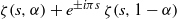 $\zeta (s, \alpha )+ {e}^{\pm i\pi s} \hspace{0.167em} \zeta (s, 1- \alpha )$ of Hurwitz zeta functions has no zeros in
  $s$ for all
  $0\leq \alpha \leq 1$ . This problem is motivated by the construction of fundamental cardinal splines of complex order
  $s$ .
$s$ .


Computing zeta functions of nondegenerate hypersurfaces with few monomials
- Part of
-
- Journal:
- LMS Journal of Computation and Mathematics / Volume 16 / October 2013
- Published online by Cambridge University Press:
- 14 February 2013, pp. 9-44
-
- Article
-
- You have access
- Export citation
A comprehensive perturbation theorem for estimating magnitudes of roots of polynomials
-
- Journal:
- LMS Journal of Computation and Mathematics / Volume 16 / October 2013
- Published online by Cambridge University Press:
- 14 February 2013, pp. 1-8
-
- Article
-
- You have access
- Export citation
References
-
- Book:
- Generalized Vectorization, Cross-Products, and Matrix Calculus
- Published online:
- 05 February 2013
- Print publication:
- 11 February 2013, pp 257-258
-
- Chapter
- Export citation
Two - Zero-One Matrices
-
- Book:
- Generalized Vectorization, Cross-Products, and Matrix Calculus
- Published online:
- 05 February 2013
- Print publication:
- 11 February 2013, pp 28-88
-
- Chapter
- Export citation
Three - Elimination and Duplication Matrices
-
- Book:
- Generalized Vectorization, Cross-Products, and Matrix Calculus
- Published online:
- 05 February 2013
- Print publication:
- 11 February 2013, pp 89-133
-
- Chapter
- Export citation
Generalized Vectorization, Cross-Products, and Matrix Calculus - Title page
-
-
- Book:
- Generalized Vectorization, Cross-Products, and Matrix Calculus
- Published online:
- 05 February 2013
- Print publication:
- 11 February 2013, pp iii-iii
-
- Chapter
- Export citation
Symbols and Operators Used in this Book
-
- Book:
- Generalized Vectorization, Cross-Products, and Matrix Calculus
- Published online:
- 05 February 2013
- Print publication:
- 11 February 2013, pp 255-256
-
- Chapter
- Export citation
Index
-
- Book:
- Generalized Vectorization, Cross-Products, and Matrix Calculus
- Published online:
- 05 February 2013
- Print publication:
- 11 February 2013, pp 259-267
-
- Chapter
- Export citation
One - Mathematical Prerequisites
-
- Book:
- Generalized Vectorization, Cross-Products, and Matrix Calculus
- Published online:
- 05 February 2013
- Print publication:
- 11 February 2013, pp 1-27
-
- Chapter
- Export citation
Six - Applications
-
- Book:
- Generalized Vectorization, Cross-Products, and Matrix Calculus
- Published online:
- 05 February 2013
- Print publication:
- 11 February 2013, pp 214-254
-
- Chapter
- Export citation
Generalized Vectorization, Cross-Products, and Matrix Calculus - Half title page
-
- Book:
- Generalized Vectorization, Cross-Products, and Matrix Calculus
- Published online:
- 05 February 2013
- Print publication:
- 11 February 2013, pp i-ii
-
- Chapter
- Export citation
Contents
-
- Book:
- Generalized Vectorization, Cross-Products, and Matrix Calculus
- Published online:
- 05 February 2013
- Print publication:
- 11 February 2013, pp v-viii
-
- Chapter
- Export citation
Four - Matrix Calculus
-
- Book:
- Generalized Vectorization, Cross-Products, and Matrix Calculus
- Published online:
- 05 February 2013
- Print publication:
- 11 February 2013, pp 134-163
-
- Chapter
- Export citation
