Refine search
Actions for selected content:
53182 results in Statistics and Probability
Frontmatter
-
- Book:
- A Practical Guide to Data Analysis Using R
- Published online:
- 11 May 2024
- Print publication:
- 30 May 2024, pp i-iv
-
- Chapter
- Export citation
3 - Laplacian eigenvalues and optimality
-
-
- Book:
- Groups and Graphs, Designs and Dynamics
- Published online:
- 11 May 2024
- Print publication:
- 30 May 2024, pp 176-265
-
- Chapter
- Export citation
Contents
-
- Book:
- Groups and Graphs, Designs and Dynamics
- Published online:
- 11 May 2024
- Print publication:
- 30 May 2024, pp v-x
-
- Chapter
- Export citation
7 - Multilevel Models, and Repeated Measures
-
- Book:
- A Practical Guide to Data Analysis Using R
- Published online:
- 11 May 2024
- Print publication:
- 30 May 2024, pp 318-372
-
- Chapter
- Export citation
4 - Exploiting the Linear Model Framework
-
- Book:
- A Practical Guide to Data Analysis Using R
- Published online:
- 11 May 2024
- Print publication:
- 30 May 2024, pp 208-244
-
- Chapter
- Export citation
Index of R Functions
-
- Book:
- A Practical Guide to Data Analysis Using R
- Published online:
- 11 May 2024
- Print publication:
- 30 May 2024, pp 514-518
-
- Chapter
- Export citation
Counting spanning subgraphs in dense hypergraphs
- Part of
-
- Journal:
- Combinatorics, Probability and Computing / Volume 33 / Issue 6 / November 2024
- Published online by Cambridge University Press:
- 30 May 2024, pp. 729-741
-
- Article
- Export citation
-
We give a simple method to estimate the number of distinct copies of some classes of spanning subgraphs in hypergraphs with a high minimum degree. In particular, for each
 $k\geq 2$ and
  $1\leq \ell \leq k-1$, we show that every
  $k$-graph on
  $n$ vertices with minimum codegree at leastcontains
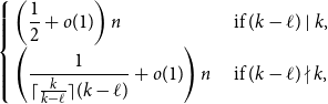 \begin{equation*} \left \{\begin {array}{l@{\quad}l} \left (\dfrac {1}{2}+o(1)\right )n & \text { if }(k-\ell )\mid k,\\[5pt] \left (\dfrac {1}{\lceil \frac {k}{k-\ell }\rceil (k-\ell )}+o(1)\right )n & \text { if }(k-\ell )\nmid k, \end {array} \right . \end{equation*}
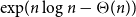 $\exp\!(n\log n-\Theta (n))$ Hamilton
  $\ell$-cycles as long as
  $(k-\ell )\mid n$. When
  $(k-\ell )\mid k$, this gives a simple proof of a result of Glock, Gould, Joos, Kühn, and Osthus, while when
  $(k-\ell )\nmid k$, this gives a weaker count than that given by Ferber, Hardiman, and Mond, or when
  $\ell \lt k/2$, by Ferber, Krivelevich, and Sudakov, but one that holds for an asymptotically optimal minimum codegree bound.


Frontmatter
-
- Book:
- Groups and Graphs, Designs and Dynamics
- Published online:
- 11 May 2024
- Print publication:
- 30 May 2024, pp i-iv
-
- Chapter
- Export citation
Author Index
-
- Book:
- Groups and Graphs, Designs and Dynamics
- Published online:
- 11 May 2024
- Print publication:
- 30 May 2024, pp 423-426
-
- Chapter
- Export citation
Dedication
-
- Book:
- A Practical Guide to Data Analysis Using R
- Published online:
- 11 May 2024
- Print publication:
- 30 May 2024, pp v-vi
-
- Chapter
- Export citation
Appendix A - The R System: a Brief Overview
-
- Book:
- A Practical Guide to Data Analysis Using R
- Published online:
- 11 May 2024
- Print publication:
- 30 May 2024, pp 469-494
-
- Chapter
- Export citation
4 - Symbolic dynamics and the stable algebra of matrices
-
-
- Book:
- Groups and Graphs, Designs and Dynamics
- Published online:
- 11 May 2024
- Print publication:
- 30 May 2024, pp 266-422
-
- Chapter
- Export citation
6 - Time Series Models
-
- Book:
- A Practical Guide to Data Analysis Using R
- Published online:
- 11 May 2024
- Print publication:
- 30 May 2024, pp 292-317
-
- Chapter
- Export citation
Index of Terms
-
- Book:
- A Practical Guide to Data Analysis Using R
- Published online:
- 11 May 2024
- Print publication:
- 30 May 2024, pp 519-526
-
- Chapter
- Export citation
Authors
-
- Book:
- Groups and Graphs, Designs and Dynamics
- Published online:
- 11 May 2024
- Print publication:
- 30 May 2024, pp xi-xii
-
- Chapter
- Export citation
2 - Quantum probability approach to spectral analysis of growing graphs
-
-
- Book:
- Groups and Graphs, Designs and Dynamics
- Published online:
- 11 May 2024
- Print publication:
- 30 May 2024, pp 87-175
-
- Chapter
- Export citation
References
-
- Book:
- A Practical Guide to Data Analysis Using R
- Published online:
- 11 May 2024
- Print publication:
- 30 May 2024, pp 495-507
-
- Chapter
- Export citation
2 - Generalizing from Models
-
- Book:
- A Practical Guide to Data Analysis Using R
- Published online:
- 11 May 2024
- Print publication:
- 30 May 2024, pp 88-143
-
- Chapter
- Export citation
Subject Index
-
- Book:
- Groups and Graphs, Designs and Dynamics
- Published online:
- 11 May 2024
- Print publication:
- 30 May 2024, pp 427-434
-
- Chapter
- Export citation
Preface
-
- Book:
- A Practical Guide to Data Analysis Using R
- Published online:
- 11 May 2024
- Print publication:
- 30 May 2024, pp xvii-xxiv
-
- Chapter
- Export citation
