Refine search
Actions for selected content:
53194 results in Statistics and Probability
On mappings on the hypercube with small average stretch
- Part of
-
- Journal:
- Combinatorics, Probability and Computing / Volume 32 / Issue 2 / March 2023
- Published online by Cambridge University Press:
- 18 October 2022, pp. 334-348
-
- Article
- Export citation
-
Let
 $A \subseteq \{0,1\}^n$ be a set of size
  $2^{n-1}$, and let
  $\phi \,:\, \{0,1\}^{n-1} \to A$ be a bijection. We define the average stretch of
  $\phi$ aswhere the expectation is taken over uniformly random
 \begin{equation*} {\sf avgStretch}(\phi ) = {\mathbb E}[{{\sf dist}}(\phi (x),\phi (x'))], \end{equation*}
 $x,x' \in \{0,1\}^{n-1}$ that differ in exactly one coordinate.
In this paper, we continue the line of research studying mappings on the discrete hypercube with small average stretch. We prove the following results.
For any set
 $A \subseteq \{0,1\}^n$ of density
  $1/2$ there exists a bijection
  $\phi _A \,:\, \{0,1\}^{n-1} \to A$ such that
  ${\sf avgStretch}(\phi _A) = O\left(\sqrt{n}\right)$.
For
 $n = 3^k$ let
  ${A_{\textsf{rec-maj}}} = \{x \in \{0,1\}^n \,:\,{\textsf{rec-maj}}(x) = 1\}$, where
 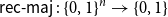 ${\textsf{rec-maj}} \,:\, \{0,1\}^n \to \{0,1\}$ is the function recursive majority of 3’s. There exists a bijection
 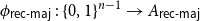 $\phi _{{\textsf{rec-maj}}} \,:\, \{0,1\}^{n-1} \to{A_{\textsf{rec-maj}}}$ such that
  ${\sf avgStretch}(\phi _{{\textsf{rec-maj}}}) = O(1)$.
Let
 ${A_{{\sf tribes}}} = \{x \in \{0,1\}^n \,:\,{\sf tribes}(x) = 1\}$. There exists a bijection
 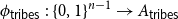 $\phi _{{\sf tribes}} \,:\, \{0,1\}^{n-1} \to{A_{{\sf tribes}}}$ such that
  ${\sf avgStretch}(\phi _{{\sf tribes}}) = O(\!\log (n))$.
These results answer the questions raised by Benjamini, Cohen, and Shinkar (Isr. J. Math 2016).


KERNEL ESTIMATION OF SPOT VOLATILITY WITH MICROSTRUCTURE NOISE USING PRE-AVERAGING
-
- Journal:
- Econometric Theory / Volume 40 / Issue 3 / June 2024
- Published online by Cambridge University Press:
- 18 October 2022, pp. 558-607
-
- Article
- Export citation
ANALYSIS OF GLOBAL AND LOCAL OPTIMA OF REGULARIZED QUANTILE REGRESSION IN HIGH DIMENSIONS: A SUBGRADIENT APPROACH
-
- Journal:
- Econometric Theory / Volume 40 / Issue 2 / April 2024
- Published online by Cambridge University Press:
- 18 October 2022, pp. 233-277
-
- Article
- Export citation
-
Regularized quantile regression (QR) is a useful technique for analyzing heterogeneous data under potentially heavy-tailed error contamination in high dimensions. This paper provides a new analysis of the estimation/prediction error bounds of the global solution of
 $L_1$-regularized QR (QR-LASSO) and the local solutions of nonconvex regularized QR (QR-NCP) when the number of covariates is greater than the sample size. Our results build upon and significantly generalize the earlier work in the literature. For certain heavy-tailed error distributions and a general class of design matrices, the least-squares-based LASSO cannot achieve the near-oracle rate derived under the normality assumption no matter the choice of the tuning parameter. In contrast, we establish that QR-LASSO achieves the near-oracle estimation error rate for a broad class of models under conditions weaker than those in the literature. For QR-NCP, we establish the novel results that all local optima within a feasible region have desirable estimation accuracy. Our analysis applies to not just the hard sparsity setting commonly used in the literature, but also to the soft sparsity setting which permits many small coefficients. Our approach relies on a unified characterization of the global/local solutions of regularized QR via subgradients using a generalized Karush–Kuhn–Tucker condition. The theory of the paper establishes a key property of the subdifferential of the quantile loss function in high dimensions, which is of independent interest for analyzing other high-dimensional nonsmooth problems.

Multisystem inflammatory syndrome associated with SARS-CoV-2 infection in children: update and new insights from the second report of an Iranian referral hospital
-
- Journal:
- Epidemiology & Infection / Volume 150 / 2022
- Published online by Cambridge University Press:
- 18 October 2022, e179
-
- Article
-
- You have access
- Open access
- HTML
- Export citation
Digital twinning of self-sensing structures using the statistical finite element method
-
- Journal:
- Data-Centric Engineering / Volume 3 / 2022
- Published online by Cambridge University Press:
- 17 October 2022, e31
-
- Article
-
- You have access
- Open access
- HTML
- Export citation
-
The monitoring of infrastructure assets using sensor networks is becoming increasingly prevalent. A digital twin in the form of a finite element (FE) model, as commonly used in design and construction, can help make sense of the copious amount of collected sensor data. This paper demonstrates the application of the statistical finite element method (statFEM), which provides a principled means of synthesizing data and physics-based models, in developing a digital twin of a self-sensing structure. As a case study, an instrumented steel railway bridge of
 $ 27.34\hskip1.5pt \mathrm{m} $ length located along the West Coast Mainline near Staffordshire in the UK is considered. Using strain data captured from fiber Bragg grating sensors at 108 locations along the bridge superstructure, statFEM can predict the “true” system response while taking into account the uncertainties in sensor readings, applied loading, and FE model misspecification errors. Longitudinal strain distributions along the two main I-beams are both measured and modeled during the passage of a passenger train. The statFEM digital twin is able to generate reasonable strain distribution predictions at locations where no measurement data are available, including at several points along the main I-beams and on structural elements on which sensors are not even installed. The implications for long-term structural health monitoring and assessment include optimization of sensor placement and performing more reliable what-if analyses at locations and under loading scenarios for which no measurement data are available.

A Hermite spline approach for modelling population mortality
-
- Journal:
- Annals of Actuarial Science / Volume 17 / Issue 2 / July 2023
- Published online by Cambridge University Press:
- 17 October 2022, pp. 243-284
-
- Article
- Export citation
Inheritance of strong mixing and weak dependence under renewal sampling
- Part of
-
- Journal:
- Journal of Applied Probability / Volume 60 / Issue 2 / June 2023
- Published online by Cambridge University Press:
- 14 October 2022, pp. 435-451
- Print publication:
- June 2023
-
- Article
- Export citation
-
Let X be a continuous-time strongly mixing or weakly dependent process and let T be a renewal process independent of X. We show general conditions under which the sampled process
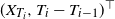 $(X_{T_i},T_i-T_{i-1})^{\top}$ is strongly mixing or weakly dependent. Moreover, we explicitly compute the strong mixing or weak dependence coefficients of the renewal sampled process and show that exponential or power decay of the coefficients of X is preserved (at least asymptotically). Our results imply that essentially all central limit theorems available in the literature for strongly mixing or weakly dependent processes can be applied when renewal sampled observations of the process X are at our disposal.

Know Your Customer: Balancing innovation and regulation for financial inclusion
-
- Journal:
- Data & Policy / Volume 4 / 2022
- Published online by Cambridge University Press:
- 14 October 2022, e34
-
- Article
-
- You have access
- Open access
- HTML
- Export citation
“Pension decumulation pathways: A proposed approach” by the Pension Decumulation Pathways Working Party
-
- Journal:
- British Actuarial Journal / Volume 27 / 2022
- Published online by Cambridge University Press:
- 14 October 2022, e20
-
- Article
-
- You have access
- Open access
- HTML
- Export citation
Large deviations of Poisson Telecom processes
- Part of
-
- Journal:
- Journal of Applied Probability / Volume 60 / Issue 1 / March 2023
- Published online by Cambridge University Press:
- 12 October 2022, pp. 267-283
- Print publication:
- March 2023
-
- Article
- Export citation
-
We study large-deviation probabilities of Telecom processes appearing as limits in a critical regime of the infinite-source Poisson model elaborated by I. Kaj and M. Taqqu. We examine three different regimes of large deviations (LD) depending on the deviation level. A Telecom process
 $(Y_t)_{t \ge 0}$ scales as
  $t^{1/\gamma}$, where t denotes time and
  $\gamma\in(1,2)$ is the key parameter of Y. We must distinguish moderate LD
  ${\mathbb P}(Y_t\ge y_t)$ with
  $t^{1/\gamma} \ll y_t \ll t$, intermediate LD with
  $ y_t \approx t$, and ultralarge LD with
  $ y_t \gg t$. The results we obtain essentially depend on another parameter of Y, namely the resource distribution. We solve completely the cases of moderate and intermediate LD (the latter being the most technical one), whereas the ultralarge deviation asymptotics is found for the case of regularly varying distribution tails. In all the cases considered, the large-deviation level is essentially reached by the minimal necessary number of ‘service processes’.


Dispersive orderings induced by differences of inter risk measures
- Part of
-
- Journal:
- Journal of Applied Probability / Volume 60 / Issue 1 / March 2023
- Published online by Cambridge University Press:
- 12 October 2022, pp. 358-365
- Print publication:
- March 2023
-
- Article
- Export citation
Food security analysis and forecasting: A machine learning case study in southern Malawi
-
- Journal:
- Data & Policy / Volume 4 / 2022
- Published online by Cambridge University Press:
- 11 October 2022, e33
-
- Article
-
- You have access
- Open access
- HTML
- Export citation
Graph distances in scale-free percolation: the logarithmic case
- Part of
-
- Journal:
- Journal of Applied Probability / Volume 60 / Issue 1 / March 2023
- Published online by Cambridge University Press:
- 11 October 2022, pp. 295-313
- Print publication:
- March 2023
-
- Article
- Export citation
-
Scale-free percolation is a stochastic model for complex networks. In this spatial random graph model, vertices
 $x,y\in\mathbb{Z}^d$ are linked by an edge with probability depending on independent and identically distributed vertex weights and the Euclidean distance
  $|x-y|$. Depending on the various parameters involved, we get a rich phase diagram. We study graph distance and compare it to the Euclidean distance of the vertices. Our main attention is on a regime where graph distances are (poly-)logarithmic in the Euclidean distance. We obtain improved bounds on the logarithmic exponents. In the light tail regime, the correct exponent is identified.


CONSISTENT SPECIFICATION TESTING UNDER SPATIAL DEPENDENCE
-
- Journal:
- Econometric Theory / Volume 40 / Issue 2 / April 2024
- Published online by Cambridge University Press:
- 11 October 2022, pp. 278-319
-
- Article
-
- You have access
- Open access
- Export citation
Human leukocyte antigen distributions do not share a copula across sub-populations
-
- Journal:
- Experimental Results / Volume 3 / 2022
- Published online by Cambridge University Press:
- 10 October 2022, e24
-
- Article
-
- You have access
- Open access
- HTML
- Export citation
Design of a Ni-based superalloy for laser repair applications using probabilistic neural network identification
-
- Journal:
- Data-Centric Engineering / Volume 3 / 2022
- Published online by Cambridge University Press:
- 10 October 2022, e30
-
- Article
-
- You have access
- Open access
- HTML
- Export citation
A transport process on graphs and its limiting distributions
- Part of
-
- Journal:
- Journal of Applied Probability / Volume 60 / Issue 1 / March 2023
- Published online by Cambridge University Press:
- 10 October 2022, pp. 341-357
- Print publication:
- March 2023
-
- Article
- Export citation
-
Given a finite strongly connected directed graph
 $G=(V, E)$, we study a Markov chain taking values on the space of probability measures on V. The chain, motivated by biological applications in the context of stochastic population dynamics, is characterized by transitions between states that respect the structure superimposed by E: mass (probability) can only be moved between neighbors in G. We provide conditions for the ergodicity of the chain. In a simple, symmetric case, we fully characterize the invariant probability.

Eliminating proxy errors from capital estimates by targeted exact computation
-
- Journal:
- Annals of Actuarial Science / Volume 17 / Issue 2 / July 2023
- Published online by Cambridge University Press:
- 07 October 2022, pp. 219-242
-
- Article
-
- You have access
- Open access
- HTML
- Export citation
Epidemiology and bacterial characteristics of invasive group B streptococcus disease: a population-based study in Japan in 2010–2020
-
- Journal:
- Epidemiology & Infection / Volume 150 / 2022
- Published online by Cambridge University Press:
- 07 October 2022, e184
-
- Article
-
- You have access
- Open access
- HTML
- Export citation
Anomalous recurrence of Markov chains on negatively curved manifolds
- Part of
-
- Journal:
- Journal of Applied Probability / Volume 60 / Issue 1 / March 2023
- Published online by Cambridge University Press:
- 06 October 2022, pp. 204-222
- Print publication:
- March 2023
-
- Article
- Export citation
