Refine search
Actions for selected content:
212758 results in Engineering
Hydrogen bonding in the crystal structure of molnupiravir Form I, C13H19N3O7
-
- Journal:
- Powder Diffraction / Volume 40 / Issue 1 / March 2025
- Published online by Cambridge University Press:
- 16 January 2025, pp. 72-75
-
- Article
-
- You have access
- Open access
- HTML
- Export citation
1 - Mathematical Optimization
-
- Book:
- Hands-On Mathematical Optimization with Python
- Published online:
- 14 May 2025
- Print publication:
- 16 January 2025, pp 1-14
-
- Chapter
- Export citation
7 - Accounting for Uncertainty: Optimization Meets Reality
-
- Book:
- Hands-On Mathematical Optimization with Python
- Published online:
- 14 May 2025
- Print publication:
- 16 January 2025, pp 203-212
-
- Chapter
- Export citation
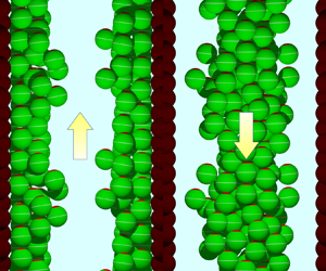
Poiseuille flow of a concentrated suspension of squirmers
-
- Journal:
- Journal of Fluid Mechanics / Volume 1003 / 25 January 2025
- Published online by Cambridge University Press:
- 16 January 2025, A23
-
- Article
-
- You have access
- Open access
- HTML
- Export citation
Figures
-
- Book:
- Hands-On Mathematical Optimization with Python
- Published online:
- 14 May 2025
- Print publication:
- 16 January 2025, pp x-xiii
-
- Chapter
- Export citation
References
-
- Book:
- Hands-On Mathematical Optimization with Python
- Published online:
- 14 May 2025
- Print publication:
- 16 January 2025, pp 331-332
-
- Chapter
- Export citation
9 - Stochastic Optimization
-
- Book:
- Hands-On Mathematical Optimization with Python
- Published online:
- 14 May 2025
- Print publication:
- 16 January 2025, pp 239-264
-
- Chapter
- Export citation
Preface
-
- Book:
- Hands-On Mathematical Optimization with Python
- Published online:
- 14 May 2025
- Print publication:
- 16 January 2025, pp xvii-xviii
-
- Chapter
- Export citation
Tables
-
- Book:
- Hands-On Mathematical Optimization with Python
- Published online:
- 14 May 2025
- Print publication:
- 16 January 2025, pp xiv-xvi
-
- Chapter
- Export citation
10 - Two-Stage Problems
-
- Book:
- Hands-On Mathematical Optimization with Python
- Published online:
- 14 May 2025
- Print publication:
- 16 January 2025, pp 265-308
-
- Chapter
- Export citation
Copyright page
-
- Book:
- Hands-On Mathematical Optimization with Python
- Published online:
- 14 May 2025
- Print publication:
- 16 January 2025, pp iv-iv
-
- Chapter
- Export citation
Generation of radioisotopes for medical applications using high-repetition, high-intensity lasers
-
- Journal:
- High Power Laser Science and Engineering / Volume 13 / 2025
- Published online by Cambridge University Press:
- 16 January 2025, e11
-
- Article
-
- You have access
- Open access
- HTML
- Export citation
-
We used the PW high-repetition laser facility VEGA-3 at Centro de Láseres Pulsados in Salamanca, with the goal of studying the generation of radioisotopes using laser-driven proton beams. Various types of targets have been irradiated, including in particular several targets containing boron to generate α-particles through the hydrogen–boron fusion reaction. We have successfully identified γ-ray lines from several radioisotopes created by irradiation using laser-generated α-particles or protons including 43Sc, 44Sc, 48Sc, 7Be, 11C and 18F. We show that radioisotope generation can be used as a diagnostic tool to evaluate α-particle generation in laser-driven proton–boron fusion experiments. We also show the production of 11C radioisotopes,
 $\approx 6 \times 10^{6}$, and of 44Sc radioisotopes,
  $\approx 5 \times 10^{4}$ per laser shot. This result can open the way to develop laser-driven radiation sources of radioisotopes for medical applications.


Alfvén waves at low magnetic Reynolds number: transitions between diffusion, dispersive Alfvén waves and nonlinear propagation
-
- Journal:
- Journal of Fluid Mechanics / Volume 1003 / 25 January 2025
- Published online by Cambridge University Press:
- 16 January 2025, A19
-
- Article
-
- You have access
- Open access
- HTML
- Export citation
-
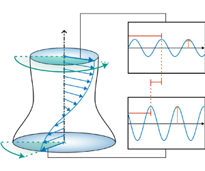
We seek the conditions in which Alfvén waves (AW) can be produced in laboratory-scale liquid metal experiments, i.e. at low magnetic Reynolds Number (
 $Rm$). Alfvén waves are incompressible waves propagating along magnetic fields typically found in geophysical and astrophysical systems. Despite the high values of
  $Rm$ in these flows, AW can undergo high dissipation in thin regions, for example in the solar corona where anomalous heating occurs (Davila, Astrophys. J., vol. 317, 1987, p. 514; Singh & Subramanian, Sol. Phys., vol. 243, 2007, pp. 163–169). Understanding how AW dissipate energy and studying their nonlinear regime in controlled laboratory conditions may thus offer a convenient alternative to observations to understand these mechanisms at a fundamental level. Until now, however, only linear waves have been experimentally produced in liquid metals because of the large magnetic dissipation they undergo when
  $Rm\ll 1$ and the conditions of their existence at low
  $Rm$ are not understood. To address these questions, we force AW with an alternating electric current in a liquid metal in a transverse magnetic field. We provide the first mathematical derivation of a wave-bearing extension of the usual low-
 $Rm$ magnetohydrodynamics (MHD) approximation to identify two linear regimes: the purely diffusive regime exists when
  $N_{\omega }$, the ratio of the oscillation period to the time scale of diffusive two-dimensionalisation by the Lorentz force, is small; the propagative regime is governed by the ratio of the forcing period to the AW propagation time scale, which we call the Jameson number
  $Ja$ after (Jameson, J. Fluid Mech., vol. 19, issue 4, 1964, pp. 513–527). In this regime, AW are dissipative and dispersive as they propagate more slowly where transverse velocity gradients are higher. Both regimes are recovered in the FlowCube experiment (Pothérat & Klein, J. Fluid Mech., vol. 761, 2014, pp. 168–205), in excellent agreement with the model up to
  $Ja \lesssim 0.85$ but near the
  $Ja=1$ resonance, high amplitude waves become clearly nonlinear. Hence, in electrically driving AW, we identified the purely diffusive MHD regime, the regime where linear, dispersive AW propagate, and the regime of nonlinear propagation.


4 - Network Optimization
-
- Book:
- Hands-On Mathematical Optimization with Python
- Published online:
- 14 May 2025
- Print publication:
- 16 January 2025, pp 91-129
-
- Chapter
- Export citation
Effects of X-ray pre-ablation on the implosion process for double-cone ignition
- Part of
-
- Journal:
- High Power Laser Science and Engineering / Volume 13 / 2025
- Published online by Cambridge University Press:
- 16 January 2025, e24
-
- Article
-
- You have access
- Open access
- HTML
- Export citation
6 - Conic Optimization
-
- Book:
- Hands-On Mathematical Optimization with Python
- Published online:
- 14 May 2025
- Print publication:
- 16 January 2025, pp 174-202
-
- Chapter
- Export citation

Turbulent kinetic energy budget in compressible turbulent mixing layers: effects of large-scale structures
-
- Journal:
- Journal of Fluid Mechanics / Volume 1003 / 25 January 2025
- Published online by Cambridge University Press:
- 16 January 2025, A25
-
- Article
- Export citation
-
Direct numerical simulations of temporally developing compressible mixing layers have been performed to investigate the effects of large-scale structures (LSSs) on turbulent kinetic energy (TKE) budgets at convective Mach numbers ranging from
 $M_c=0.2$ to
  $1.8$ and at Taylor Reynolds numbers up to 290. In the core region of mixing layers, the volume fraction of low-speed LSSs decreases linearly with respect to the vertical distance at a Mach-number-independent rate. The contributions of low-speed LSSs to TKE, and its budget, including production, dissipation, pressure-strain and spatial diffusion terms, are primarily concentrated in the upper region of mixing layer. The streamwise and vertical mass flux coupling terms mainly transport TKE downwards in low-speed LSSs, and their magnitudes are comparable to the other dominant terms. Near the edges of LSSs, the sources and losses of all three components of TKE are completely different to each other, and dominated by turbulent diffusion, pressure diffusion, pressure-strain and dissipation terms. The TKE, their total variation and dissipation are significantly amplified at edges of low-speed LSSs, especially at the upper edge. This observation supports the existence of amplitude modulation exerted by the LSSs onto the near-edge small-scale structures in mixing layers. The level of amplitude modulation is strongest for the vertical velocity, followed by the streamwise velocity, and weakest for the spanwise velocity. Additionally, the amplitude modulation effect decreases significantly with increasing convective Mach number. The results on the amplitude modulation effect is helpful for developing predictive models of budget terms of TKE in mixing layers.


Hydrodynamic diffusion in apolar active suspensions of squirmers
-
- Journal:
- Journal of Fluid Mechanics / Volume 1003 / 25 January 2025
- Published online by Cambridge University Press:
- 16 January 2025, A17
-
- Article
-
- You have access
- Open access
- HTML
- Export citation

Pressure fluctuations of liquids under short-time acceleration
-
- Journal:
- Journal of Fluid Mechanics / Volume 1003 / 25 January 2025
- Published online by Cambridge University Press:
- 16 January 2025, A20
-
- Article
-
- You have access
- Open access
- HTML
- Export citation
-
This study investigates experimentally the pressure fluctuations of liquids in a column under short-time acceleration. It demonstrates that the Strouhal number
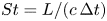 $St=L/(c\,\Delta t)$, where
  $L$,
$L$,  $c$ and
  $\Delta t$ are the liquid column length, speed of sound, and acceleration duration, respectively, provides a measure of the pressure fluctuations for intermediate
  $St$ values. On the one hand, the incompressible fluid theory implies that the magnitude of the averaged pressure fluctuation
  $\bar {P}$ becomes negligible for
  $St\ll 1$. On the other hand, the water hammer theory predicts that the pressure tends to
  $\rho cu_0$ (where
  $u_0$ is the change in the liquid velocity) for
  $St\geq O(1)$. For intermediate
  $St$ values, there is no consensus on the value of
  $\bar {P}$. In our experiments,
  $L$,
$L$,  $c$ and
  $\Delta t$ are varied so that
 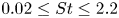 $0.02 \leq St \leq 2.2$. The results suggest that the incompressible fluid theory holds only up to
  $St\sim 0.2$, and that
  $St$ governs the pressure fluctuations under different experimental conditions for higher
  $St$ values. The data relating to a hydrogel also tend to collapse to a unified trend. The inception of cavitation in the liquid starts at
  $St\sim 0.2$ for various
  $\Delta t$, indicating that the liquid pressure goes lower than the liquid vapour pressure. To understand this mechanism, we employ a one-dimensional wave propagation model with a pressure wavefront of finite thickness that scales with
  $\Delta t$. The model provides a reasonable description of the experimental results as a function of
  $St$.
$St$.


3 - Mixed-Integer Linear Optimization
-
- Book:
- Hands-On Mathematical Optimization with Python
- Published online:
- 14 May 2025
- Print publication:
- 16 January 2025, pp 48-90
-
- Chapter
- Export citation
