Refine search
Actions for selected content:
26077 results in Abstract analysis
Asymptotic properties of the solutions to stochastic KPP equations
-
- Journal:
- Proceedings of the Royal Society of Edinburgh. Section A: Mathematics / Volume 130 / Issue 6 / December 2000
- Published online by Cambridge University Press:
- 11 July 2007, pp. 1363-1381
- Print publication:
- December 2000
-
- Article
- Export citation
Uniqueness of positive radial solutions of a semilinear Dirichlet problem in an annulus
-
- Journal:
- Proceedings of the Royal Society of Edinburgh. Section A: Mathematics / Volume 130 / Issue 6 / December 2000
- Published online by Cambridge University Press:
- 11 July 2007, pp. 1417-1428
- Print publication:
- December 2000
-
- Article
- Export citation
The convexity of the spectral function in Sturm–Liouville problems
- Part of
-
- Journal:
- Mathematika / Volume 47 / Issue 1-2 / December 2000
- Published online by Cambridge University Press:
- 26 February 2010, pp. 319-326
- Print publication:
- December 2000
-
- Article
- Export citation
-
§1. Introduction. The spectral function ρα(μ) (−∞<μ<∞) associated with the Sturm–Liouville equation

and a boundary condition

is a non-decreasing function of μ which is defined in terms of the Titchmarsh–Weyl function mα(λ) for (1.1) and (1.2).
N-fold sums of Cantor sets
- Part of
-
- Journal:
- Mathematika / Volume 47 / Issue 1-2 / December 2000
- Published online by Cambridge University Press:
- 26 February 2010, pp. 243-250
- Print publication:
- December 2000
-
- Article
- Export citation
Character sums with exponential functions
- Part of
-
- Journal:
- Mathematika / Volume 47 / Issue 1-2 / December 2000
- Published online by Cambridge University Press:
- 26 February 2010, pp. 75-85
- Print publication:
- December 2000
-
- Article
- Export citation
-
Let ϑ be an integer of multiplicative order t≥1 modulo a prime p. Sums of the form
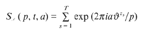
are introduced and estimated, with
 a sequence such that kz1, …, kzT is a permutation of z1, …, zT, both sequences taken modulo t, for sufficiently many distinct modulo t values of k. Such sequences include
xn for x = 1 ,…,t with an integer n≥1;
xn for x = 1 ,…,t and gcd (x, t) = 1 with an integer n≥1;
ex for x = 1 ,…,T with an integer e, where T is the period of the sequence ex modulo t.
Some of the results can be extended to composite moduli and to sums of multiplicative characters as well. Character sums with the above sequences have some cryptographic motivation and applications and have been considered in several papers by J. B. Friedlander, D. Lieman and I. E. Shparlinski. In particular several previous bounds are generalized and improved.
 a sequence such that kz
The order of inverses mod q
- Part of
-
- Journal:
- Mathematika / Volume 47 / Issue 1-2 / December 2000
- Published online by Cambridge University Press:
- 26 February 2010, pp. 87-108
- Print publication:
- December 2000
-
- Article
- Export citation
-
Let q be a prime number and let a = (a1, …, as) be an s-tuple of distinct integers modulo q. For any x coprime with q, let
 be such that
  . For fixed s and q→∞ an asymptotic formula is given for the number of residue classes x modulo q for which
The more general case, when q is not necessarily prime and x is restricted to lie in a given subinterval of [1, q], is also treated.
 be such that
  . For fixed s and q→∞ an asymptotic formula is given for the number of residue classes x modulo q for which
On the Wielandt length of a finite supersoluble group
-
- Journal:
- Proceedings of the Royal Society of Edinburgh. Section A: Mathematics / Volume 130 / Issue 6 / December 2000
- Published online by Cambridge University Press:
- 11 July 2007, pp. 1217-1226
- Print publication:
- December 2000
-
- Article
- Export citation
Index to volume 47
-
- Journal:
- Mathematika / Volume 47 / Issue 1-2 / December 2000
- Published online by Cambridge University Press:
- 26 February 2010, pp. 411-412
- Print publication:
- December 2000
-
- Article
- Export citation
The order of groups satisfying a converse to Lagrange's theorem
- Part of
-
- Journal:
- Mathematika / Volume 47 / Issue 1-2 / December 2000
- Published online by Cambridge University Press:
- 26 February 2010, pp. 197-204
- Print publication:
- December 2000
-
- Article
- Export citation
On properties of metrizable spaces X preserved by t-equivalence
- Part of
-
- Journal:
- Mathematika / Volume 47 / Issue 1-2 / December 2000
- Published online by Cambridge University Press:
- 26 February 2010, pp. 273-279
- Print publication:
- December 2000
-
- Article
- Export citation
Density and covering properties of intervals of ℝn
- Part of
-
- Journal:
- Mathematika / Volume 47 / Issue 1-2 / December 2000
- Published online by Cambridge University Press:
- 26 February 2010, pp. 229-242
- Print publication:
- December 2000
-
- Article
- Export citation
-
The key result of this paper proves the existence of functions ρn(h) for which, whenever H is a (Lebesgue) measurable subset of the n-dimensional unit cube In with measure |H| > h and ℛ is a class of subintervals (n-dimensional axis-parallel rectangles) of In that covers H, then there exists an interval R∈ℛ in which the density of H is greater than ρn(h); that is, |H∩R|/|R|>ρn (h) (=(h/2n)2). It is shown how to use this result to find 4 points of a measurable subset of the unit square which are the vertices of an axis-parallel rectangle that has quite large intersection with the original set. Density and covering properties of classes of subsets of ℝn are introduced and investigated. As a consequence, a covering property of the class of intervals of ℝn is obtained: if ℛ is a family of n-dimensional intervals with
 , then there is a finite sequence R1, …, Rm∈ℛ such that
  and
and  .
.
 , then there is a finite sequence R
 and
and  .
.Bh [g] sequences
- Part of
-
- Journal:
- Mathematika / Volume 47 / Issue 1-2 / December 2000
- Published online by Cambridge University Press:
- 26 February 2010, pp. 109-115
- Print publication:
- December 2000
-
- Article
- Export citation
-
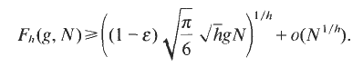
New upper and lower bounds are given for Fh(g, N), the maximum size of a Bh[g] sequence contained in [1, N]. It is proved that and that

and that, for any ε > 0 and g > g(ε, h),
Multiple solutions for semilinear elliptic problems
- Part of
-
- Journal:
- Mathematika / Volume 47 / Issue 1-2 / December 2000
- Published online by Cambridge University Press:
- 26 February 2010, pp. 307-317
- Print publication:
- December 2000
-
- Article
- Export citation
Fubini-type theorems for general measure constructions
- Part of
-
- Journal:
- Mathematika / Volume 47 / Issue 1-2 / December 2000
- Published online by Cambridge University Press:
- 26 February 2010, pp. 251-265
- Print publication:
- December 2000
-
- Article
- Export citation
Inequalities for the Hurwitz zeta function
-
- Journal:
- Proceedings of the Royal Society of Edinburgh. Section A: Mathematics / Volume 130 / Issue 6 / December 2000
- Published online by Cambridge University Press:
- 11 July 2007, pp. 1227-1236
- Print publication:
- December 2000
-
- Article
- Export citation
-
Let
be the Hurwitz zeta function. Furthermore, let p > 1 and α ≠ 0 be real numbers and n ≥ 2 be an integer. We determine the best possible constants a(p, α, n), A(p, α, n), b(p, n) and B(p, n) such that the inequalities
 and
and hold for all positive real numbers x1,…,xn.
Segments in ball packings
- Part of
-
- Journal:
- Mathematika / Volume 47 / Issue 1-2 / December 2000
- Published online by Cambridge University Press:
- 26 February 2010, pp. 31-38
- Print publication:
- December 2000
-
- Article
- Export citation
Vortex structures for an SO(5) model of high-TC superconductivity and antiferromagnetism
-
- Journal:
- Proceedings of the Royal Society of Edinburgh. Section A: Mathematics / Volume 130 / Issue 6 / December 2000
- Published online by Cambridge University Press:
- 11 July 2007, pp. 1183-1215
- Print publication:
- December 2000
-
- Article
- Export citation
Regularity and propagation of moments in some nonlinear Vlasov systems
-
- Journal:
- Proceedings of the Royal Society of Edinburgh. Section A: Mathematics / Volume 130 / Issue 6 / December 2000
- Published online by Cambridge University Press:
- 11 July 2007, pp. 1259-1273
- Print publication:
- December 2000
-
- Article
- Export citation
Additive representation in thin sequences, II: The binary Goldbach problem
- Part of
-
- Journal:
- Mathematika / Volume 47 / Issue 1-2 / December 2000
- Published online by Cambridge University Press:
- 26 February 2010, pp. 117-125
- Print publication:
- December 2000
-
- Article
- Export citation
Dynamics of the diffusive Nicholson's blowflies equation with distributed delay
-
- Journal:
- Proceedings of the Royal Society of Edinburgh. Section A: Mathematics / Volume 130 / Issue 6 / December 2000
- Published online by Cambridge University Press:
- 11 July 2007, pp. 1275-1291
- Print publication:
- December 2000
-
- Article
- Export citation
