Refine search
Actions for selected content:
238152 results in Physics and Astronomy

Direct numerical simulations of bubble-mediated gas transfer and dissolution in quiescent and turbulent flows
-
- Journal:
- Journal of Fluid Mechanics / Volume 954 / 10 January 2023
- Published online by Cambridge University Press:
- 06 January 2023, A29
-
- Article
-
- You have access
- Open access
- HTML
- Export citation
-
We perform direct numerical simulations of a gas bubble dissolving in a surrounding liquid. The bubble volume is reduced due to dissolution of the gas, with the numerical implementation of an immersed boundary method, coupling the gas diffusion and the Navier–Stokes equations. The methods are validated against planar and spherical geometries’ analytical moving boundary problems, including the classic Epstein–Plesset problem. Considering a bubble rising in a quiescent liquid, we show that the mass transfer coefficient
 $k_L$ can be described by the classic Levich formula
  $k_L = (2/\sqrt {{\rm \pi} })\sqrt {\mathscr {D}_l\,U(t)/d(t)}$, with
  $d(t)$ and
  $U(t)$ the time-varying bubble size and rise velocity, and
  $\mathscr {D}_l$ the gas diffusivity in the liquid. Next, we investigate the dissolution and gas transfer of a bubble in homogeneous and isotropic turbulence flow, extending Farsoiya et al. (J. Fluid Mech., vol. 920, 2021, A34). We show that with a bubble size initially within the turbulent inertial subrange, the mass transfer coefficient in turbulence
  $k_L$ is controlled by the smallest scales of the flow, the Kolmogorov
  $\eta$ and Batchelor
  $\eta _B$ microscales, and is independent of the bubble size. This leads to the non-dimensional transfer rate
  ${Sh}=k_L L^\star /\mathscr {D}_l$ scaling as
  ${Sh}/{Sc}^{1/2} \propto {Re}^{3/4}$, where
  ${Re}$ is the macroscale Reynolds number
  ${Re} = u_{rms}L^\star /\nu _l$, with
  $u_{rms}$ the velocity fluctuations,
  $L^*$ the integral length scale,
  $\nu _l$ the liquid viscosity, and
  ${Sc}=\nu _l/\mathscr {D}_l$ the Schmidt number. This scaling can be expressed in terms of the turbulence dissipation rate
  $\epsilon$ as
 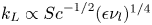 ${k_L}\propto {Sc}^{-1/2} (\epsilon \nu _l)^{1/4}$, in agreement with the model proposed by Lamont & Scott (AIChE J., vol. 16, issue 4, 1970, pp. 513–519) and corresponding to the high
  $Re$ regime from Theofanous et al. (Intl J. Heat Mass Transfer, vol. 19, issue 6, 1976, pp. 613–624).


Laser wakefield accelerator modelling with variational neural networks
- Part of
-
- Journal:
- High Power Laser Science and Engineering / Volume 11 / 2023
- Published online by Cambridge University Press:
- 06 January 2023, e9
-
- Article
-
- You have access
- Open access
- HTML
- Export citation
The reduction of pressure losses in thermally modulated vertical channels
-
- Journal:
- Journal of Fluid Mechanics / Volume 954 / 10 January 2023
- Published online by Cambridge University Press:
- 06 January 2023, A38
-
- Article
-
- You have access
- Open access
- HTML
- Export citation
Two- and three-dimensional wake transitions of a NACA0012 airfoil
-
- Journal:
- Journal of Fluid Mechanics / Volume 954 / 10 January 2023
- Published online by Cambridge University Press:
- 06 January 2023, A26
-
- Article
-
- You have access
- Open access
- HTML
- Export citation
-
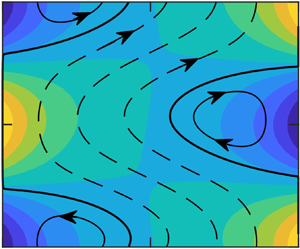
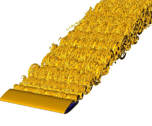
Flow transitions are an important fluid-dynamic phenomena for many reasons, including the direct effect on the aerodynamic forces acting on the body. In the present study, two-dimensional (2-D) and three-dimensional (3-D) wake transitions of a NACA0012 airfoil are studied for angles of attack in the range
 $0^\circ \leq \alpha \leq 20^\circ$ and Reynolds numbers
  $500 \leq {\textit {Re}} \leq 5000$. The study uses water-channel experiments and 2-D and 3-D numerical simulations based on the nodal spectral-element method, level-set function-based immersed-interface method and Floquet stability analysis. The different wake states are categorised based on the time-instantaneous wake structure, non-dimensional frequency and aerodynamic force coefficients. The wake states and transition boundaries are summarised in a wake regime map. The critical angle of attack and Reynolds number for the supercritical Hopf bifurcation (i.e. steady to periodic wake transition) varies as
  $\alpha _1 {\sim} {\textit {Re}}^{-0.65}$, while the critical angle of attack for the onset of three dimensionality varies as
  $\alpha _{3D} {\sim} {\textit {Re}}^{-0.5}$. Over the entire Reynolds number range, the transition to 3-D flow occurs through a mode C (subharmonic) transition. Beyond this initial transition, further instabilities of the 2-D periodic base flow arise and are investigated. For instance, at
  $ {\textit {Re}}=2000$ and
  $\alpha _{3D,2}=11.0^\circ$, mode C coexists together with modes related to modes A and QP seen in a stationary circular cylinder wake. In contrast, at
  $ {\textit {Re}}=5000$ and
  $\alpha _{3D,2}=8.0^\circ$, the dominant mode C coexists with mode QP. Three-dimensional simulations well beyond critical angles indicate that 2-D vortex-street transitions are approximately maintained in the fully saturated 3-D wakes in a spanwise-averaged sense.


The role of Lagrangian drift in the geometry, kinematics and dynamics of surface waves
-
- Journal:
- Journal of Fluid Mechanics / Volume 954 / 10 January 2023
- Published online by Cambridge University Press:
- 06 January 2023, R4
-
- Article
-
- You have access
- Open access
- HTML
- Export citation
Chapter Five - Percolation on ℤ𝑑
-
- Book:
- Network Models for Data Science
- Published online:
- 22 March 2023
- Print publication:
- 05 January 2023, pp 105-135
-
- Chapter
- Export citation
15 - Mesoscopic Effects
- from Part IV - Disordered Metals and Superconductors
-
- Book:
- Field Theory of Non-Equilibrium Systems
- Published online:
- 15 January 2023
- Print publication:
- 05 January 2023, pp 370-390
-
- Chapter
- Export citation
II - Basic Phenomenology of Magnetism
-
- Book:
- Experimental Techniques in Magnetism and Magnetic Materials
- Published online:
- 27 October 2022
- Print publication:
- 05 January 2023, pp 19-22
-
- Chapter
- Export citation
6 - Special Functions
-
- Book:
- Computing in Scilab
- Published online:
- 15 October 2023
- Print publication:
- 05 January 2023, pp 259-284
-
- Chapter
- Export citation
4 - Ordinary Differential Equation
-
- Book:
- Computing in Scilab
- Published online:
- 15 October 2023
- Print publication:
- 05 January 2023, pp 135-228
-
- Chapter
- Export citation
6 - Digital Holography
-
- Book:
- Modern Information Optics with MATLAB
- Published online:
- 22 December 2022
- Print publication:
- 05 January 2023, pp 190-259
-
- Chapter
- Export citation
Frontmatter
-
- Book:
- Continuous Groups for Physicists
- Published online:
- 24 November 2022
- Print publication:
- 05 January 2023, pp i-iv
-
- Chapter
- Export citation
Subject Index
-
- Book:
- Network Models for Data Science
- Published online:
- 22 March 2023
- Print publication:
- 05 January 2023, pp 477-484
-
- Chapter
- Export citation
Frontmatter
-
- Book:
- Field Theory of Non-Equilibrium Systems
- Published online:
- 15 January 2023
- Print publication:
- 05 January 2023, pp i-iv
-
- Chapter
- Export citation
List of Figures
-
- Book:
- Computing in Scilab
- Published online:
- 15 October 2023
- Print publication:
- 05 January 2023, pp xi-xvi
-
- Chapter
- Export citation
Chapter Six - Percolation Beyond ℤ𝑑
-
- Book:
- Network Models for Data Science
- Published online:
- 22 March 2023
- Print publication:
- 05 January 2023, pp 136-160
-
- Chapter
- Export citation
-
Summary
Percolation can be defined more generally than as a process on
,
Chapter Sixteen - Graphons as Limits of Networks
-
- Book:
- Network Models for Data Science
- Published online:
- 22 March 2023
- Print publication:
- 05 January 2023, pp 393-410
-
- Chapter
- Export citation
1 - Introduction
-
- Book:
- Field Theory of Non-Equilibrium Systems
- Published online:
- 15 January 2023
- Print publication:
- 05 January 2023, pp 1-8
-
- Chapter
- Export citation
Chapter Fifteen - Examining Network Properties
-
- Book:
- Network Models for Data Science
- Published online:
- 22 March 2023
- Print publication:
- 05 January 2023, pp 374-392
-
- Chapter
- Export citation
Index
-
- Book:
- Continuous Groups for Physicists
- Published online:
- 24 November 2022
- Print publication:
- 05 January 2023, pp 277-280
-
- Chapter
- Export citation
