Refine search
Actions for selected content:
212937 results in Engineering
9 - Optimization Basics and Logistic Regression
-
- Book:
- Linear Algebra for Data Science, Machine Learning, and Signal Processing
- Published online:
- 01 November 2024
- Print publication:
- 16 May 2024, pp 335-364
-
- Chapter
- Export citation
3 - Matrix Factorization: Eigendecomposition and SVD
-
- Book:
- Linear Algebra for Data Science, Machine Learning, and Signal Processing
- Published online:
- 01 November 2024
- Print publication:
- 16 May 2024, pp 63-95
-
- Chapter
- Export citation

Jetting enhancement from wall-proximal cavitation bubbles by a distant wall
-
- Journal:
- Journal of Fluid Mechanics / Volume 987 / 25 May 2024
- Published online by Cambridge University Press:
- 16 May 2024, R2
-
- Article
-
- You have access
- Open access
- HTML
- Export citation
-
An additional distant wall is known to highly alter the jetting scenarios of wall-proximal bubbles. Here, we combine high-speed photography and axisymmetric volume of fluid (VoF) simulations to quantitatively describe its role in enhancing the micro-jet dynamics within the directed jet regime (Zeng et al., J. Fluid Mech., vol. 896, 2020, A28). Upon a favourable agreement on the bubble and micro-jet dynamics, both experimental and simulation results indicate that the micro-jet velocity increases dramatically as
 $\eta$ decreases, where
  $\eta =H/R_{max}$ is the distance between two walls
  $H$ normalized by the maximum bubble radius
  $R_{max}$. The mechanism is related to the collapsing flow, which is constrained by the distant wall into a reverse stagnation-point flow that builds up pressure near the bubble's top surface and accelerates it into micro-jets. We further derive an equation expressing the micro-jet velocity
  $U_{jet}=87.94\gamma ^{0.5}(1+(1/3)(\eta -\lambda ^{1.2})^{-2})$, where
  ${\gamma =d/R_{max}}$ is the stand-off distance to the proximal wall with
  $d$ the distance between the initial bubble centre and the wall,
 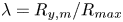 $\lambda =R_{y,m}/R_{max}$ with
  $R_{y,m}$ the distance between the top surface and the proximal wall at the bubble's maximum expansion. Viscosity has a minimal impact on the jet velocity for small
  $\gamma$, where the pressure buildup is predominantly influenced by geometry.


FLM volume 986 Cover and Front matter
-
- Journal:
- Journal of Fluid Mechanics / Volume 986 / 10 May 2024
- Published online by Cambridge University Press:
- 16 May 2024, p. f1
-
- Article
-
- You have access
- Export citation
Preface
-
- Book:
- Linear Algebra for Data Science, Machine Learning, and Signal Processing
- Published online:
- 01 November 2024
- Print publication:
- 16 May 2024, pp xv-xviii
-
- Chapter
- Export citation
2 - Introduction to Matrices
-
- Book:
- Linear Algebra for Data Science, Machine Learning, and Signal Processing
- Published online:
- 01 November 2024
- Print publication:
- 16 May 2024, pp 12-62
-
- Chapter
- Export citation

What are the immediate standards needs for quantum technology?
-
- Journal:
- Research Directions: Quantum Technologies / Volume 2 / 2024
- Published online by Cambridge University Press:
- 16 May 2024, e2
-
- Article
-
- You have access
- Open access
- HTML
- Export citation
Copyright page
-
- Book:
- Linear Algebra for Data Science, Machine Learning, and Signal Processing
- Published online:
- 01 November 2024
- Print publication:
- 16 May 2024, pp iv-iv
-
- Chapter
- Export citation
Stability of a dispersion of elongated particles embedded in a viscous membrane
-
- Journal:
- Journal of Fluid Mechanics / Volume 987 / 25 May 2024
- Published online by Cambridge University Press:
- 16 May 2024, R4
-
- Article
-
- You have access
- Open access
- HTML
- Export citation
5 - Linear Least-Squares Regression and Binary Classification
-
- Book:
- Linear Algebra for Data Science, Machine Learning, and Signal Processing
- Published online:
- 01 November 2024
- Print publication:
- 16 May 2024, pp 143-196
-
- Chapter
- Export citation
12 - Random Matrix Theory, Signal + Noise Matrices, and Phase Transitions
-
- Book:
- Linear Algebra for Data Science, Machine Learning, and Signal Processing
- Published online:
- 01 November 2024
- Print publication:
- 16 May 2024, pp 390-404
-
- Chapter
- Export citation
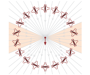
Polymers in turbulence: any better than dumbbells?
-
- Journal:
- Journal of Fluid Mechanics / Volume 987 / 25 May 2024
- Published online by Cambridge University Press:
- 16 May 2024, R1
-
- Article
-
- You have access
- Open access
- HTML
- Export citation
11 - Neural Network Models
-
- Book:
- Linear Algebra for Data Science, Machine Learning, and Signal Processing
- Published online:
- 01 November 2024
- Print publication:
- 16 May 2024, pp 381-389
-
- Chapter
- Export citation
1 - Getting Started
-
- Book:
- Linear Algebra for Data Science, Machine Learning, and Signal Processing
- Published online:
- 01 November 2024
- Print publication:
- 16 May 2024, pp 1-11
-
- Chapter
- Export citation
Acknowledgments
-
- Book:
- Linear Algebra for Data Science, Machine Learning, and Signal Processing
- Published online:
- 01 November 2024
- Print publication:
- 16 May 2024, pp xix-xx
-
- Chapter
- Export citation
10 - Matrix Completion and Recommender Systems
-
- Book:
- Linear Algebra for Data Science, Machine Learning, and Signal Processing
- Published online:
- 01 November 2024
- Print publication:
- 16 May 2024, pp 365-380
-
- Chapter
- Export citation
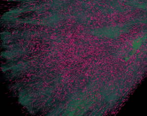
Stability of Stuart vortices in rotating stratified fluids
-
- Journal:
- Journal of Fluid Mechanics / Volume 987 / 25 May 2024
- Published online by Cambridge University Press:
- 16 May 2024, A12
-
- Article
- Export citation
Dedication
-
- Book:
- Linear Algebra for Data Science, Machine Learning, and Signal Processing
- Published online:
- 01 November 2024
- Print publication:
- 16 May 2024, pp v-vi
-
- Chapter
- Export citation

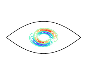
Coexistence of dual wing–wake interaction mechanisms during the rapid rotation of flapping wings
-
- Journal:
- Journal of Fluid Mechanics / Volume 987 / 25 May 2024
- Published online by Cambridge University Press:
- 16 May 2024, A16
-
- Article
- Export citation
-
Insects flip their wings around each stroke reversal and may enhance lift in the early stage of a half-stroke. The possible lift-enhancing mechanism of this rapid wing rotation and its strong connection with wake vortices are still underexplored, especially when unsteady leading-edge vortex (LEV) behaviours occur. Here, we numerically studied the lift generation and underlying vorticity dynamics during the rapid rotation of a low aspect ratio flapping wing at a Reynolds number (
 ${\textit {Re}}$) of 1500. Our findings prove that when the outboard LEV breaks down, an advanced rotation can still enhance the lift in the early stage of a half-stroke, which originates from an interaction with the breakdown vortex in the outboard region. This interaction, named the breakdown-vortex jet mechanism, results in a jet and thus a higher pressure on the upwind surface, including a stronger wingtip suction force on the leeward surface. Although the stable LEV within the mid-span retains its growth and location during an advanced rotation, it can be detrimental to lift enhancement as it moves underneath the wing. Therefore, for a flapping wing at
  ${\textit {Re}}\sim 10^3$, the interactions with stable and breakdown leading-edge vortices lead to the single-vortex suction and breakdown-vortex jet mechanisms, respectively. In other words, the contribution of wing–wake interaction depends on the spanwise location. The current work also implies the importance of wing kinematics to this wing–wake interaction in flapping wings, and provides an alternative perspective for understanding this complex flow phenomenon at
  ${\textit {Re}}\sim 10^3$.


6 - Norms and Procrustes Problems
-
- Book:
- Linear Algebra for Data Science, Machine Learning, and Signal Processing
- Published online:
- 01 November 2024
- Print publication:
- 16 May 2024, pp 197-237
-
- Chapter
- Export citation
