Refine search
Actions for selected content:
212971 results in Engineering
A.4 - Physical Constants
- from Appendices
-
- Book:
- Integrated Circuit Fabrication
- Published online:
- 01 December 2023
- Print publication:
- 16 November 2023, pp 643-643
-
- Chapter
- Export citation
2 - Fuzzy Sets and Fuzzy Logic
-
- Book:
- Introduction to Intelligent Systems, Control, and Machine Learning using MATLAB
- Published online:
- 27 November 2023
- Print publication:
- 16 November 2023, pp 16-59
-
- Chapter
- Export citation
1 - What Is an Intelligent System?
-
- Book:
- Introduction to Intelligent Systems, Control, and Machine Learning using MATLAB
- Published online:
- 27 November 2023
- Print publication:
- 16 November 2023, pp 1-15
-
- Chapter
- Export citation
A.1 - Basics of Semiconductor Materials in Equilibrium
- from Appendices
-
- Book:
- Integrated Circuit Fabrication
- Published online:
- 01 December 2023
- Print publication:
- 16 November 2023, pp 619-640
-
- Chapter
- Export citation
8 - Deep Learning
-
- Book:
- Introduction to Intelligent Systems, Control, and Machine Learning using MATLAB
- Published online:
- 27 November 2023
- Print publication:
- 16 November 2023, pp 252-322
-
- Chapter
- Export citation
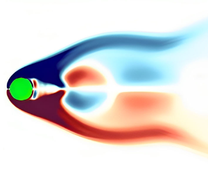
Significant influence of fluid viscoelasticity on flow dynamics past an oscillating cylinder
-
- Journal:
- Journal of Fluid Mechanics / Volume 975 / 25 November 2023
- Published online by Cambridge University Press:
- 16 November 2023, A26
-
- Article
- Export citation
-
This study focuses on numerically investigating the impact of fluid viscoelasticity on the flow dynamics around a transversely forced oscillating cylinder operating in the laminar vortex shedding regime at a fixed Reynolds number of $Re = 100$. Specifically, we explore how fluid viscoelasticity affects the boundary between the lock-in and no lock-in regions and the corresponding wake characteristics compared with a simple Newtonian fluid. Our findings reveal that fluid viscoelasticity enables the synchronization of the vortex street with the cylinder motion at lower oscillation frequencies than those required for a Newtonian fluid. Consequently, the lock-in region boundary for a viscoelastic fluid differs from that of a Newtonian fluid and expands in the non-dimensional cylinder oscillation amplitude and frequency parameter space. In the primary synchronization region, the wake of a Newtonian fluid exhibits ‘2S’ (two single vortices) and ‘P+S’ (a pair of vortices and a single vortex) shedding modes. In contrast, a ‘2P’ (two pairs of vortices) vortex mode is observed for a viscoelastic fluid within the same region. To gain a deeper understanding of the differences in the coherent flow structures and their associated frequencies between the two fluids, we employ the data-driven reduced-order modelling technique, known as the dynamic mode decomposition (DMD) technique. Utilizing this technique, we successfully extract and visualize the two competing fundamental frequencies (cylinder oscillation and natural vortex shedding frequencies) and their associated flow structures in the case of the no lock-in state, whereas only the dominant cylinder oscillation frequency and associated flow structure in the case of the lock-in state. Furthermore, we propose that the presence of excess strain resulting from the stretching of polymer molecules in viscoelastic fluids leads to a distinct difference in the wake structure compared with Newtonian fluids. This observation aligns with the findings obtained from the $Q$-criterion and vorticity transport analysis of the wake.


1 - Introduction
-
- Book:
- Cryptoeconomics
- Published online:
- 06 January 2024
- Print publication:
- 16 November 2023, pp 1-20
-
- Chapter
- Export citation
Appendix A - Modern Control System Tutorial
-
- Book:
- Introduction to Intelligent Systems, Control, and Machine Learning using MATLAB
- Published online:
- 27 November 2023
- Print publication:
- 16 November 2023, pp 375-404
-
- Chapter
- Export citation
Appendix B - MATLAB Tutorial
-
- Book:
- Introduction to Intelligent Systems, Control, and Machine Learning using MATLAB
- Published online:
- 27 November 2023
- Print publication:
- 16 November 2023, pp 405-422
-
- Chapter
- Export citation
2 - Modern Complementary Metal-Oxide–Semiconductor (CMOS) Technology
-
- Book:
- Integrated Circuit Fabrication
- Published online:
- 01 December 2023
- Print publication:
- 16 November 2023, pp 37-69
-
- Chapter
- Export citation
7 - Doping in Semiconductors
-
- Book:
- Integrated Circuit Fabrication
- Published online:
- 01 December 2023
- Print publication:
- 16 November 2023, pp 310-379
-
- Chapter
- Export citation
Dedication
-
- Book:
- Introduction to Intelligent Systems, Control, and Machine Learning using MATLAB
- Published online:
- 27 November 2023
- Print publication:
- 16 November 2023, pp v-vi
-
- Chapter
- Export citation
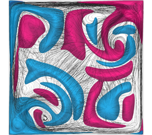
Wall mode dynamics and transition to chaos in magnetoconvection with a vertical magnetic field
-
- Journal:
- Journal of Fluid Mechanics / Volume 975 / 25 November 2023
- Published online by Cambridge University Press:
- 16 November 2023, R2
-
- Article
- Export citation
-
Quasistatic magnetoconvection of a fluid with low Prandtl number ( ${\textit {Pr}}=0.025$) with a vertical magnetic field is considered in a unit-aspect-ratio box with no-slip boundaries. At high relative magnetic field strengths, given by the Hartmann number ${\textit {Ha}}$, the onset of convection is known to result from a sidewall instability giving rise to the wall-mode regime. Here, we carry out three-dimensional direct numerical simulations of unprecedented length to map out the parameter space at ${\textit {Ha}} = 200, 500, 1000$, varying the Rayleigh number ( ${\textit {Ra}}$) over the range $6\times 10^5 \lesssim {\textit {Ra}} \lesssim 5\times 10^8$. We track the development of stable equilibria produced by this primary instability, identifying bifurcations leading to limit cycles and eventually to chaotic dynamics. At ${\textit {Ha}}=200$, the steady wall-mode solution undergoes a symmetry-breaking bifurcation producing a state that features a coexistence between wall modes and a large-scale roll in the centre of the domain, which persists to higher ${\textit {Ra}}$. However, under a stronger magnetic field at ${\textit {Ha}}=1000$, the steady wall-mode solution undergoes a Hopf bifurcation producing a limit cycle which further develops to solutions that shadow an orbit homoclinic to a saddle point. Upon a further increase in ${\textit {Ra}}$, the system undergoes a subsequent symmetry break producing a coexistence between wall modes and a large-scale roll, although the large-scale roll exists only for a small range of ${\textit {Ra}}$, and chaotic dynamics primarily arise from a mixture of chaotic wall-mode dynamics and arrays of cellular structures.


Part II - Consensus Protocol Design in Blockchain Networks
-
- Book:
- Cryptoeconomics
- Published online:
- 06 January 2024
- Print publication:
- 16 November 2023, pp 51-52
-
- Chapter
- Export citation
Copyright page
-
- Book:
- Introduction to Intelligent Systems, Control, and Machine Learning using MATLAB
- Published online:
- 27 November 2023
- Print publication:
- 16 November 2023, pp iv-iv
-
- Chapter
- Export citation

Jet from a very large, axisymmetric, surface-gravity wave
-
- Journal:
- Journal of Fluid Mechanics / Volume 975 / 25 November 2023
- Published online by Cambridge University Press:
- 16 November 2023, A22
-
- Article
-
- You have access
- Open access
- HTML
- Export citation
-
We demonstrate that gravity acting alone at large length scales (compared to the capillary length) can produce a jet from a sufficiently steep, axisymmetric surface deformation imposed on a quiescent, deep pool of liquid. Mechanistically, the jet owes it origin to the focusing of a concentric, surface wave towards the axis of symmetry, quite analogous to such focusing of capillary waves and resultant jet formation observed during bubble collapse at small scales. A weakly nonlinear theory based on the method of multiple scales in the potential flow limit is presented for a modal (single-mode) initial condition representing the solution to the primary Cauchy–Poisson problem. A pair of novel, coupled, amplitude equations are derived governing the modulation of the primary mode. For moderate values of the perturbation parameter $\epsilon$ (a measure of the initial perturbation steepness), our second-order theory captures the overshoot (incipient jet) at the axis of symmetry quite well, demonstrating good agreement with numerical simulation of the incompressible, Euler equation with gravity (Popinet 2014, Basilisk. http://basilisk.fr) and no surface tension. We demonstrate that the underlying wave focusing mechanism may be understood in terms of radially inward motion of nodal points of a linearised, axisymmetric, standing wave. This explanation rationalises the ubiquitous observation of such jets accompanying cavity collapse phenomena, spanning length scales from microns to several metres. Expectedly, our theory becomes inaccurate as $\epsilon$ approaches unity. In this strongly nonlinear regime, slender jets form with surface accelerations exceeding gravity by more than an order of magnitude. In this inertial regime, we compare the jets in our simulations with the inertial, self-similar, analytical solution by Longuet-Higgins (J. Fluid Mech., 1983, vol. 127, pp. 103–121) and find qualitative agreement with the same. This analysis demonstrates, from first principles, an example of a jet created purely under gravity from a smooth initial perturbation and provides support to the analytical model of Longuet-Higgins (J. Fluid Mech., 1983, vol. 127, pp. 103–121).


Dedication
-
- Book:
- Cryptoeconomics
- Published online:
- 06 January 2024
- Print publication:
- 16 November 2023, pp v-vi
-
- Chapter
- Export citation
4 - Optimization: Hard Computing
-
- Book:
- Introduction to Intelligent Systems, Control, and Machine Learning using MATLAB
- Published online:
- 27 November 2023
- Print publication:
- 16 November 2023, pp 109-141
-
- Chapter
- Export citation
Appendix F - Programming Microcontrollers with Simulink and Support Package
-
- Book:
- Introduction to Intelligent Systems, Control, and Machine Learning using MATLAB
- Published online:
- 27 November 2023
- Print publication:
- 16 November 2023, pp 463-466
-
- Chapter
- Export citation
Contents
-
- Book:
- Cryptoeconomics
- Published online:
- 06 January 2024
- Print publication:
- 16 November 2023, pp vii-viii
-
- Chapter
- Export citation
