In this paper, we study the converse of comparison results for solutions to linear second-order elliptic equations. Namely, in the inequalities proved by G. Talenti and others, we study the case of equality and prove that “equalities are achieved only in the spherical situation”. We also present some applications of these results to semilinear elliptic equations.

We consider the equations for the isothermal motion of a one-dimensional unbounded body composed of a material with viscosity and capillarity. Using a technique derived from the theory of compensated compactness, we find conditions which guarantee that, as viscosity and capillarity approach zero, the solutions to these equations converge to a solution to the corresponding equations in elasticity.

In [8,9] Jayne and Rogers studied piece-wise closed maps and ℱσ maps between metric spaces. A map f of a metric space X into a metric space Y is said to be an ℱσ map if: (a) f maps ℱσ-sets in X to ℱσ-sets in Y; and (b) f1 maps ℱσ-sets in Y back to ℱσ-sets in X. A map fof a metric space X into a metric space Y is said to be piece-wise closed if:it is possible to find a sequence X1, X2,… of closed sets in X, with with each setf(Xi), i ≥ 1, closed in Y, and with the restriction offto each Xi, a closed map (i.e., a continuous map that maps closed sets to closed sets).

If E is a subset of ℝn (n ≥ 1) we define the distance set of E as

The best known result on distance sets is due to Steinhaus [11], namely, that, if E ⊂ ℝn is measurable with positive n-dimensional Lebesgue measure, then D(E) contains an interval [0, ε) for some ε > 0. A number of variations of this have been examined, see Falconer [6, p. 108] and the references cited therein.

Let A and B be Borel (or more generally Suslin) sets in ℝn whose Hausdorff dimensions satisfy

Suppose that θ is a positive irrational number and α is an arbitrary real number. Then Kronecker's Theorem in diophantine approximation (Theorem 440 of [7[) can be stated as follows.

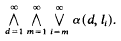
For d, n positive integers, let α(d, n) be the statement “For every abelian variety A bounded by d there exists a point P of order n”. Let l1, l2, l3, … be the sequence of prime numbers and let α be

We use the Buchstab-Rosser sieve to derive an asymptotic formula for the distribution of those integers n for which the r numbers n + l1, n + l2,…, n + lr are all square-free. Our error estimate sharpens a similar result of Hall and is uniform in both r and maxl 1≤i≤r|li|.

We consider two additive cubic equations

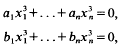
in p-adic fields. Davenport and Lewis showed that the equations have a non-trivial solution in every p-adic field, if n ≥ 16, and need not have a solution in the 7-adic field, if n = 15. Here we prove that if p ≠ 7 the equations have a non-trivial solution in p-adic fields if n ≥ 13. When n = 12 such a result fails for every prime p ≡ 1 (mod 3).

This paper considers the flow of a dissipative fluid in a radial bearing. By looking at the equations in the thermal boundary layer it is shown that, if a certain parameter m is less than unity, then the temperature in the boundary layer is bounded for all time.

Le point de départ de ce travail est le résultat suivant.

THÉORÈME (I. Namioka). Soient X et Y deux espaces compacts et

Si f est continue quand on munit(Y) de la topologie de convergence simple alors X contient un Gδ dense en tout point duquel f reste continue quand on munit(Y) de la topologie de la convergence uniform.

The work to be described here, with the fruit of previous investigations in [1] and [2], yields the following general theorem.

In 1959 C. A. Rogers gave the following estimate for the density ϑ(k) of lattice-coverings of euclidean d-space Ed with convex bodies . Here, c is a suitable constant which does not depend on d and K. Moreover, Rogers proved that for the unit ball Bd the upper bound can be replaced by , which is, of course a major improvement. In the present paper we show that such an improvement can be obtained for a larger class of convex bodies. In particular, we prove the following theorem. Let K be a convex body in Ed, and let k be an integer satisfying k > log2 loge d + 4. If there exist at least k hyperplanes H1,…, Hk with normals mutually perpendicular and an affine transformation A such that A(K) is symmetrical with respect to Hl,…,Hk, respectively, then . Actually, for a bound of this type we do not even need any symmetry assumption. In fact, some weaker properties concerning shadow boundaries will suffice.

In our paper [12[ we made extensive use of the details of the proofs given in our earlier paper [11], and, in particular, we claimed that Lemma 3 of [11] holds, not just when Y is a metric space, but also when Y is a Hausdorff space, provided X × Y is a Fréchet space. In a corrigendum to [11], we give a corrected version of this Lemma 3, but it seems to depend, in an essential way, on the assumption that Y is a metric space, or at least a perfectly normal space. In this note we show that a modified version of this Lemma 3 enables us to justify all the theorems in [12] by use of a modified method of selection.

Let be a finitely generated subgroup of SL (2, ℱ), where ℱ is the ring; of holomorphic functions on the open unit disc Δ. For each point z0 in Δ we can evaluate all matrix entries of at z0, to obtain a subgroup {z0} of SL (2, ℂ) and a surjective representation → {z0}. If this representation is not faithful, then contains a nontrivial element W such that W evaluated; at z0 is trivial. But W can evaluate to the identity only on a countable subset) of Δ, and there are only countably many choices for W in Consequently there are at most countably many points zk in Δ such that {zk} is not isomorphic to Δ. Our main result can now be stated as follows.

If E1 and E2 are subsets of ℝn and a- is an isometry or similarity transformation, it is useful to be able to estimate the Hausdorff dimension of E1 ∩ σ(E2) in terms of the dimensions of E1 and E2. If E1 and E2 are compact, then, as σvaries, dim (El ∩ σ(E2)) is “in general” at most max (dim E1 + dim E2 − n, 0) and “often” at least this value (see Mattila [9] and Kahane [7] for more precise statements of these ideas). However, as we shall see, it is possible to construct non-compact sets E of any given dimension that are “sufficiently dense” in ℝn to ensure that dim (E ∩ σ(E)) = dim E for all similarities σ More generally, we shall show that for each s there are large classes of sets & of dimensions between s and n, closed under reasonable transformations including similarities, such that the intersection of any countable collection of sets in & has dimension at least s. Such collections of sets are required, for example, in the constructions of subsets of ℝn with certain dimensional properties given by Davies [1] and Falconer [5].