In order to study weak limits of quadratic expressions of oscillatory solutions of partial differential equations, there was proposed a construction of H-measures defined on the space of positions and frequencies. The present paper is devoted to the investigation of the Tartar equationwhich describes the evolution of the H-measure μt associated with a sequence of oscillatory solutions of the linear transport equation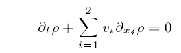in cases when a given solenoidal velocity field v(x, t) is sufficiently smooth. Here, (t, x, y) ∈ (0, T) × Ω × S1, 0 < T < +∞, Ω is a bounded open subset of R2 and S1 is the unit circle in R2, given coefficients Yij = Yij(y) are infinitely smooth.

Assuming that v belongs to , we establish the well posedness of Cauchy problem for the Tartar equation in the same measure class as the H-measures are in. For this purpose, we develop and use an extension of the theory of Lagrange coordinates for a case of non-smooth solenoidal velocity fields.

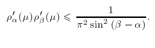
For a special case of the Sturm-Liouville equation, −(py′)′ + qy = λwy on [0, ∞) with the initial condition y(0) cos α + p(0)y′(0) sin α = 0, α ∈ [0, π), it is shown that, given the spectral derivative for two values of α ∈ [0, π) at a fixed μ = Re{λ} ≥ Λ0, it is possible to uniquely determine . An explicit formula is derived to accomplish this. Further, in a more general case of the Sturm-Liouville problem for μ with both finite and positive, then the following inequality holds

We study a boundary perturbation problem for a one-dimensional Schrödinger equation in which the potential has a regular singularity near the perturbed end point. We give the asymptotic behaviour of the eigenvalues under the perturbation. This problem arose out of the author's studies of singular elliptic operators in higher dimensions and we illustrate this point with an example. The class of potentials to which this method applies is larger than that covered by standard results, which assume uniform ellipticity of the operator or a perturbative term that is analytic in the perturbation parameter.

We prove that given a convex Jordan curve $\varGamma\subset\{x_3=0\}$, the space of properly embedded minimal annuli in the half-space $\{x_3\geq0\}$, with boundary $\varGamma$ is diffeomorphic to the interval $[0,\infty)$. Moreover, for a fixed positive number $a$, the exterior Plateau problem that consists of finding a properly embedded minimal annulus in the upper half-space, with finite total curvature, boundary $\varGamma$ and a catenoid type end with logarithmic growth $a$ has exactly zero, one or two solutions, each one with a different stability character for the Jacobi operator.

AMS 2000 Mathematics subject classification: Primary 53A10. Secondary 49Q05; 53C42

In this article we present a proof of existence of a weak solution for the semigeostrophic system of equations, formulated as an active scalar transport equation with Monge-Ampère coupling, with initial data in . This is an extension of a 1998 result due to Benamou and Brenier, who proved existence with initial data in .

Nori’s connectivity theorem compares the cohomology of $X\times B$ and $Y_B$, where $Y_B$ is any locally complete quasiprojective family of sufficiently ample complete intersections in $X$. When $X$ is the projective space, and we consider hypersurfaces of degree $d$, it is possible to give an explicit bound for $d$, sufficient to conclude that the Connectivity Theorem holds. We show that this bound is optimal, by constructing for lower $d$ classes on $Y_B$ not coming from the ambient space. As a byproduct we get the non-triviality of the higher Chow groups of generic hypersurfaces of degree $2n$ in $\mathbb{P}^{n+1}$.

AMS 2000 Mathematics subject classification: Primary 14C25; 14D07; 14J70

This is the first of three articles designed to stabilize the global trace formula. The results apply to any group for which the fundamental lemma (and its variants for weighted orbital integrals) is valid. The main purpose of this paper is to establish a series of expansions that are parallel to the expansions in the trace formula. We shall also formulate the local and global theorems required to interpret the terms in these expansions. The proofs of the theorems will be given in the subsequent two articles. The expansions of this paper will then yield both a stable trace formula, and a decomposition of the ordinary trace formula into a linear combination of stable trace formulae.

AMS 2000 Mathematics subject classification: Primary 22E55. Secondary 11R39

We present an extension of Besicovitch spaces, which has its origin in the works of Zhikov et al. and Kozlov and Oleinik. We show that these spaces have a similar behaviour to the Lp spaces, and we give a notion of derivative that allows us to treat partial differential problems in this frame. To the best of our knowledge, this is new, even for the usual Besicovitch spaces.

A necessary and sufficient geometric condition is established for the Kohn Laplacian to be hypoelliptic, modulo its nullspace, for boundaries of arbitrary infinitely differentiable pseudoconvex tube domains in two complex variables. Hypoellipticity is also proved to be equivalent to validity of a superlogarithmic estimate, for this special class of structures.

AMS 2000 Mathematics subject classification: Primary 32W05; 32T27. Secondary 35J70.

A nonlinear diffusion process modelling aggregative dispersal is combined with local (in space) population dynamics given by a logistic equation and the resulting growth-dispersal model is analysed. The nonlinear diffusion process models aggregation via a diffusion coefficient, which is decreasing with respect to the population density at low densities. This mechanism is similar to area-restricted search, but it is applied to conspecifics rather than prey. The analysis shows that in some cases the models predict a threshold effect similar to an Allee effect. That is, for some parameter ranges, the models predict a form of conditional persistence where small populations go extinct but large populations persist. This is somewhat surprising because logistic equations without diffusion or with non-aggregative diffusion predict either unconditional persistence or unconditional extinction. Furthermore, in the aggregative models, the minimum patch size needed to sustain an existing population at moderate to high densities may be smaller than the minimum patch size needed for invasibility by a small population. The tradeoff is that if a population is inhabiting a large patch whose size is reduced below the size needed to sustain any population, then the population on the patch can be expected to experience a sudden crash rather than a steady decline.

Let f : Mn×n → R ∪ {∞} be a function on the space Mn×n of n by n matrices that is invariant with respect to the left and right multiplication by proper orthogonal tensors. It is shown that f(A) ≤ f(Ā) if f is convex and the partial sums of the singular values of A, Ā ∈ Mn×n satisfy certain ordering inequalities. The same holds if f is rank 1 convex and the partial products of the singular values satisfy analogous inequalities. The proofs emphasize the roles of the ordered-forces inequalities and the Baker-Ericksen inequalities for invariant convex and rank 1 convex functions. As an application, the evaluation of the convex and lamination convex hulls of fully rotationally invariant sets by Dacorogna and Tanteri is simplified and similar results are given for sets invariant only with respect to the proper orthogonal group.

The relaxation of certain time-evolution problems is investigated. As a conceptually simple example, we study elastically deformable bodies that undergo martensitic phase transformations. The movement of the phase boundaries is hindered by dry friction. The fundamental problem is that the phase distribution forms a highly oscillatory microstructure in space. Therefore, it is desirable to derive a coarse-grained system that describes the effective properties. We introduce a concept of relaxation of the evolution system and apply it to the case where only two phases occur and the elastic energy is quadratic. Finally, we present a candidate for the relaxation in the general case.

We consider minimization problems involving the Dirichlet integral under an arbitrary number of volume constraints on the level sets and a generalized boundary condition. More precisely, given a bounded open domain Ω ⊂ Rn with smooth boundary, we study the problem of minimizing ∫Ω |∇u|2 among all those functions u ∈ H1 that simultaneously satisfy n-dimensional measure constraints on the level sets of the kind |{u = li}| = αi, i = 1,…, k, and a generalized boundary condition u ∈ K. Here, K is a closed convex subset of H1 such that ; the invariance of K under provides that the condition u ∈ K actually depends only on the trace of u along ∂Ω.

By a penalization approach, we prove the existence of minimizers and their Hölder continuity, generalizing previous results that are not applicable when a boundary condition is prescribed.

Finally, in the case of just two volume constraints, we investigate the Γ-convergence of the above (rescaled) functionals when the total measure of the two prescribed level sets tends to saturate the whole domain Ω. It turns out that the resulting Γ-limit functional can be split into two distinct parts: the perimeter of the interface due to the Dirichlet energy that concentrates along the jump, and a boundary integral term due to the constraint u ∈ K. In the particular case where K = H1 (i.e. when no boundary condition is prescribed), the boundary term vanishes and we recover a previous result due to Ambrosio et al.

Degond and Markowich discussed the existence and uniqueness of a steady-state solution in the subsonic case for the one-dimensional hydrodynamic model of semiconductors. In the present paper, we reconsider the existence and uniqueness of a globally smooth subsonic steady-state solution, and prove its stability for small perturbation. The proof method we adopt in this paper is based on elementary energy estimates.

We study a class of BGK approximations of parabolic systems in one space dimension. We prove stability and existence of global solutions for this model. Moreover, under certain conditions, we prove a rigorous result of convergence toward the formal limit, by using compensated compactness techniques.

We answer some open problems on subhereditary radicals of associative rings. In particular, we show that the Brown–McCoy radical is not subhereditary and that every left or right subhereditary and left or right stable radical satisfies all these properties. The latter of these results concerns, in fact, the question whether some classes of reduced rings are closed under one-sided essential extensions. We characterize several such classes.

On the class of labelled combinatorial structures called assemblies we define complex-valued multiplicative functions and examine their asymptotic mean values. The problem reduces to the investigation of quotients of the Taylor coefficients of exponential generating series having Euler products. Our approach, originating in probabilistic number theory, requires information on the generating functions only in the convergence disc and rather weak smoothness on the circumference. The results could be applied to studying the asymptotic value distribution of decomposable mappings defined on assemblies.

It is shown that the maximum possible chromatic number of the square of a graph with maximum degree d and girth g is (1 +o(1))d2 if g = 3, 4, 5 or 6, and is Θ(d2 / log d) if g [ges ] 7. Extensions to higher powers are considered as well.

We study the asymptotic behaviour of the relative entropy (to stationarity) for a commonly used model for riffle shuffling a deck of n cards m times. Our results establish and were motivated by a prediction in a recent numerical study of Trefethen and Trefethen. Loosely speaking, the relative entropy decays approximately linearly (in m) for m < log2n, and approximately exponentially for m > log2n. The deck becomes random in this information-theoretic sense after m = 3/2 log2n shuffles.

The circuit cover problem for mixed graphs (those containing edges and/or arcs) is defined as follows. Given a mixed graph M with a nonnegative integer weight function p on its edges and arcs, decide whether (M, p) has a circuit cover, that is, a list of circuits in M such that every edge (arc) e is contained in exactly p(e) circuits of the list. In the special case when M is a directed graph (contains only arcs), the problem is easy, but when M is an undirected graph not many results are known. For general mixed graphs this problem was shown to be NP-complete by Arkin and Papadimitriou in 1986. We prove that this problem remains NP-complete for planar mixed graphs. Furthermore, we present a good characterization for the existence of a circuit cover when M is series-parallel (a similar result holds for the fractional version). We also describe a polynomial algorithm to find such a circuit cover, when it exists. This is an ellipsoid-based algorithm whose separation problem is the minimum circuit problem on series-parallel mixed graphs, which we show to be polynomially solvable. Results on two well-known combinatorial problems, the problem of detecting negative circuits and the problem of finding shortest paths, are also presented. We prove that both problems are NP-hard for planar mixed graphs.