Refine search
Actions for selected content:
179468 results in Earth and Environmental Sciences

Transition regimes of gravity current: from salinity-driven to particle-driven
-
- Journal:
- Journal of Fluid Mechanics / Volume 1016 / 10 August 2025
- Published online by Cambridge University Press:
- 30 July 2025, A21
-
- Article
- Export citation

Revisiting Townsend’s spatial energy-density function
-
- Journal:
- Journal of Fluid Mechanics / Volume 1016 / 10 August 2025
- Published online by Cambridge University Press:
- 30 July 2025, A12
-
- Article
-
- You have access
- Open access
- HTML
- Export citation
-
Fourier analysis is the standard tool of choice for quantifying the distribution of kinetic energy amongst the eddies in a turbulent flow. The resulting spectral energy-density function is the well-known energy spectrum. And yet, because eddies are distinct from waves, alternative approaches to finding energy-density functions have long been sought. Townsend (1976) outlined a promising approach to finding a spatial energy-density function, $V\!(r)$, where $r$ is the eddy size. Notably, this approach led to two distinct and mutually inconsistent formulations of $V\!(r)$ in homogeneous, isotropic turbulence. We revisit Townsend’s proposal and derive the corresponding three-dimensional $V\!(r)$ as well as introduce its one-dimensional variants (which, to our knowledge, have not been explicitly discussed before). By training our focus on the associated dimensionality of the function, we resolve the discrepancies between the previous formulations. Additionally, we generalise our analysis to include anisotropic flows. Finally, by means of concrete examples, we illustrate how one-dimensional spatial energy-density functions are useful for analysing empirical data. Some notable findings include new insights into the $k_1^{-1}$ scaling (where $k_1$ is the streamwise wavenumber) and a possible resolution of the enigmatic sizes of organised motions at large scales.


Shock interactions on a V-shaped cowl lip at supersonic and hypersonic speeds
-
- Journal:
- Journal of Fluid Mechanics / Volume 1016 / 10 August 2025
- Published online by Cambridge University Press:
- 30 July 2025, A15
-
- Article
- Export citation
-
Shock interactions on a V-shaped blunt leading edge (VBLE) that are commonly encountered at the cowl lip of an inward-turning inlet are investigated at freestream Mach numbers ( $ M_\infty$) 3–6. The swept blunt leading edges of the VBLE generate a pair of detached shocks with varying shapes due to the changes in $ M_\infty$ and $L/r$ (i.e. the ratio of the leading-edge length $L$ to the leading-edge blunt radius $r$), which causes intriguing shock interactions at the crotch of the VBLE. Three subtypes of regular reflection (RR) and a Mach reflection (MR) are produced successively with increasing $ M_\infty$ for a given $L/r$, which appear in the opposite order to those with increasing $L/r$ for a given $ M_\infty$. These shock interactions identified in numerical simulations are verified in supersonic and hypersonic wind tunnel experiments. It is demonstrated that the relative position of the shocks is crucial in determining the transitions of shock interactions by varying either $L/r$ or $ M_\infty$. Transition criteria between subtypes of RR and from RR to MR are theoretically established in the parameter space $(M_\infty,L/r)$ by analysing the shock structures, showing good agreement with the numerical and experimental results. Interactions between either immature or fully developed detached shocks are embedded in these criteria. Specifically, the transition criteria asymptotically approach the corresponding critical $ M_\infty$ when $L/r$ is sufficiently large. These transition criteria provide guidelines for improving the design of the cowl lip of an inward-turning inlet in supersonic and hypersonic regimes.


Characterizing turbulent boundary layer response and recovery to buffer region spanwise blowing
-
- Journal:
- Journal of Fluid Mechanics / Volume 1016 / 10 August 2025
- Published online by Cambridge University Press:
- 30 July 2025, A26
-
- Article
-
- You have access
- Open access
- HTML
- Export citation
-
Experiments were performed that (i) document the effect of the steady spanwise buffer layer blowing on the mean characteristics of the turbulent boundary layer for a range of momentum thickness Reynolds numbers from 4760 to 10 386, and (ii) document the effect of the buffer layer blowing on the unsteady characteristics and coherent vorticity in a boundary layer designed to provide sufficiently high spatial resolution. The spanwise buffer layer blowing of the order of $u_{\tau }$ is produced by a surface array of pulsating direct current (pulsed-DC) plasma actuators. This was found to substantially reduce the wall shear stress that was directly measured with a floating element coupled with a force sensor. The direct wall shear measurements agreed with values derived using the Clauser method to within $\pm 0.85$ %. The degree to which the buffer layer blowing affected $\tau _w$ was found to primarily depend on the inner variable spanwise spacing between the pulsed-DC actuator electrodes, i.e. ‘blowing sites’. Utilizing pairs of $[u,v]$ and $[u,w]$ hot-wire sensors, the latter experiments correlated significant reductions in the $\omega _y$ and $\omega _x$ vorticity components that resulted from the buffer layer blowing and translated into lower Reynolds stresses and turbulence production. The time scale to which these observed changes in the boundary layer characteristics would return to the baseline condition was subsequently documented. This revealed a recovery length of $x^+ \approx 86\,000$ that translated to a streamwise fetch of $x \approx 66\delta$. Finally, a comparison with the recent work by Cheng et al. (2021, J. Fluid Mech. vol. 918, A24) and Wei & Zhou (2024 in TSFP13, June 25–28, 2024) that followed our experimental approach to achieve comparable wall shear stress (drag) reductions has led to a new scaling based on the baseline boundary layer $\textit{Re}_{\tau }$ and buffer layer blowing velocity.


Electrokinetic versus leaky-dielectric modelling of electrosprays operating in the cone-jet mode
-
- Journal:
- Journal of Fluid Mechanics / Volume 1016 / 10 August 2025
- Published online by Cambridge University Press:
- 30 July 2025, A14
-
- Article
-
- You have access
- Open access
- HTML
- Export citation
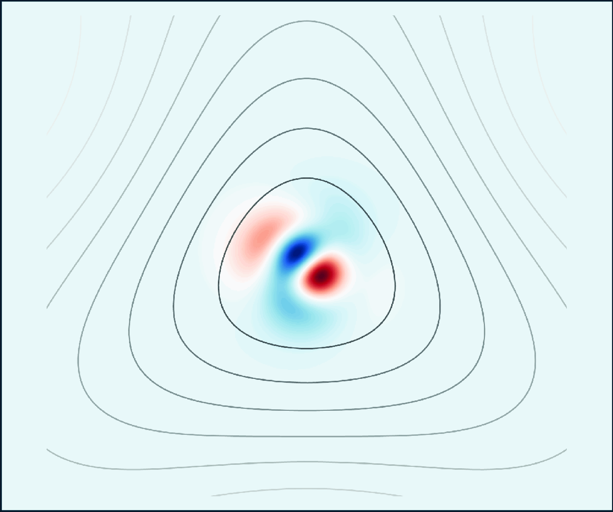
Triangular instability of a strained Lamb–Oseen vortex
-
- Journal:
- Journal of Fluid Mechanics / Volume 1016 / 10 August 2025
- Published online by Cambridge University Press:
- 29 July 2025, A9
-
- Article
-
- You have access
- Open access
- HTML
- Export citation
-
In this study, we demonstrate, for the first time, the existence of a short-wave instability in a Lamb–Oseen vortex subjected to a triangular strain field generated by three satellite vortices, which we term the triangular instability. We identify this instability by numerically integrating the linearised Navier–Stokes equations around a quasi-steady base flow to capture the most unstable mode and validate it by comparing results with theoretical predictions. We evaluate this instability by calculating the growth rates associated with the parametric resonant coupling of two Kelvin waves with the triangular strain field in the limit of small strain rate and large Reynolds number. Our analysis reveals that resonance occurs only for combinations of the azimuthal wavenumbers $m = 1$ and $m = - 2$ (or their symmetric counterparts with opposite signs). We observe several unstable modes with positive growth rates for a moderate viscous Reynolds number $10^4$ and straining parameter value $\epsilon = 0.008$, defined as the cube of the ratio of the core size to the distance from the satellite vortices. The most unstable mode, dominant at typically high Reynolds numbers, has $k \approx 5.18/a$ and $\omega \approx - 0.312\Omega$ (where $a$ and $\Omega$ denote the core size and central angular velocity). It exhibits negligible critical layer damping and remains the most unstable mode over a wide range of ${Re}$ and $\epsilon$. At lower Reynolds numbers, another mode with $k \approx 1.76/a$ and $\omega \approx - 0.407\Omega$, despite significant critical layer damping, becomes the most unstable.


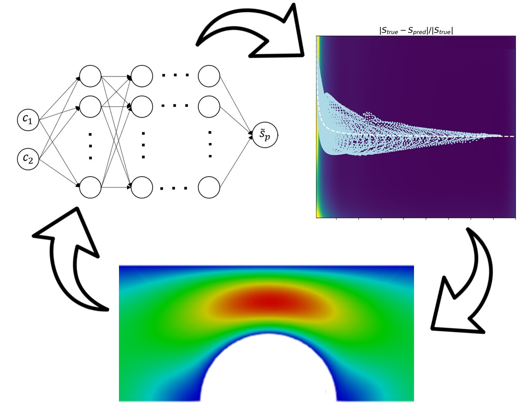
Hammering at the entropy: a GENERIC-guided approach to learning polymeric rheological constitutive equations using PINNs
-
- Journal:
- Journal of Fluid Mechanics / Volume 1016 / 10 August 2025
- Published online by Cambridge University Press:
- 29 July 2025, A11
-
- Article
-
- You have access
- Open access
- HTML
- Export citation

Double-diffusive viscous fingering induced by an active dye
-
- Journal:
- Journal of Fluid Mechanics / Volume 1016 / 10 August 2025
- Published online by Cambridge University Press:
- 29 July 2025, R3
-
- Article
- Export citation

Direct numerical simulation of power-law fluids over smooth and rough surfaces
-
- Journal:
- Journal of Fluid Mechanics / Volume 1016 / 10 August 2025
- Published online by Cambridge University Press:
- 29 July 2025, A13
-
- Article
- Export citation
-
Direct numerical simulation (DNS) studies of power-law (PL) fluids are performed for purely viscous-shear-thinning ( $n\in [0.5,0.75]$), Newtonian ( $n=1$) and purely viscous-shear-thickening ( $n=2.0$) fluids, considering two Reynolds numbers ( $Re_{\tau }\in [395,590]$), and both smooth and rough surfaces. We carefully designed a numerical experiment to isolate key effects and simplify the complex problem of turbulent flow of non-Newtonian fluids over rough surfaces, enabling the development of a theoretical model to explain the observed phenomena and provide predictions. The DNS results of the present work were validated against literature data for smooth and rough Newtonian turbulent flows, as well as smooth shear-thinning cases. A new analytical expression for the mean velocity profile – extending the classical Blasius $1/7$ profile to power-law fluids – was proposed and validated. In contrast to common belief, the decrease in $n$ leads to smaller Kolmogorov length scales and the formation of larger structures, requiring finer grids and longer computational domains for accurate simulations. Our results confirm that purely viscous shear-thinning fluids exhibit drag reduction, while shear-thickening fluids display an opposite trend. Interestingly, we found that viscous-thinning turbulence shares similarities with Newtonian transitional flows, resembling the behaviour of shear-thinning, extensional-thickening viscoelastic fluids. This observation suggests that the extensional and elastic effects in turbulent flows within constant cross-section geometries may not be significant. However, the shear-thickening case exhibits characteristics similar to high-Reynolds-number Newtonian turbulence, suggesting that phenomena observed in such flows could be studied at significantly lower Reynolds numbers, reducing computational costs. In the analysis of rough channels, we found that the recirculation bubble between two roughness elements is mildly influenced by the thinning nature of the fluid. Moreover, we observed that shear-thinning alters the flow in the fully rough regime, where the friction factor typically reaches a plateau. Our results indicate the possibility that, at sufficiently high Reynolds numbers, this plateau may not exist for shear-thinning fluids. Finally, we provide detailed turbulence statistics for different rheologies, allowing, for the first time, an in-depth study of the effects of rheology on turbulent flow over rough surfaces.


Tree semantic segmentation from aerial image time series
-
- Journal:
- Environmental Data Science / Volume 4 / 2025
- Published online by Cambridge University Press:
- 29 July 2025, e37
-
- Article
-
- You have access
- Open access
- HTML
- Export citation

Thin-layer formation of ellipsoidal gyrotactic swimmers in time-dependent hydrodynamic shear
-
- Journal:
- Journal of Fluid Mechanics / Volume 1016 / 10 August 2025
- Published online by Cambridge University Press:
- 29 July 2025, A8
-
- Article
-
- You have access
- Open access
- HTML
- Export citation
-
We investigated the dynamics of thin-layer formation by non-spherical motile phytoplankton in time-dependent shear flow, building on the seminal work of Durham et al. (2009 Science vol. 323, pp. 1067–1070), on spherical microswimmers in time-independent flows. By solving the torque balance equation for a microswimmer, we found that the system is highly damped for body sizes smaller than $10^{-3}$ m, with initial rotational motion dissipating quickly. From this torque balance, we also derived the critical shear for ellipsoidal microswimmers, which we validated numerically. Simulations revealed that the peak density of microswimmers is slightly higher than the theoretical prediction due to the speed asymmetry of sinking and gyrotaxis above and below the predicted height. In addition, we observed that microswimmers with higher aspect ratios tend to form thicker layers due to slower angular velocity. Using linear stability analysis, we identified a thin-layer accumulation time scale, which contains two regimes. This theoretically predicted accumulation time scale was validated through simulations. In time-dependent flow with oscillating critical shear depth, we identified three accumulation regimes and a transitional regime based on the ratio of swimmer and flow time scales. Our results indicate that thin layers can form across time scale ratios spanning five orders of magnitude, which helps explain the widespread occurrence of thin phytoplankton layers in natural water bodies.


Modelling transitional rough-wall turbulence with quasi-linear approximations
-
- Journal:
- Journal of Fluid Mechanics / Volume 1016 / 10 August 2025
- Published online by Cambridge University Press:
- 29 July 2025, A7
-
- Article
-
- You have access
- Open access
- HTML
- Export citation

Experimental investigation of cylindrically divergent Rayleigh–Taylor instability on a water–air interface
-
- Journal:
- Journal of Fluid Mechanics / Volume 1016 / 10 August 2025
- Published online by Cambridge University Press:
- 28 July 2025, R2
-
- Article
-
- You have access
- HTML
- Export citation

Large-eddy simulation of the fluid–structure interaction in aquatic canopies consisting of highly flexible blades
-
- Journal:
- Journal of Fluid Mechanics / Volume 1016 / 10 August 2025
- Published online by Cambridge University Press:
- 28 July 2025, A4
-
- Article
-
- You have access
- Open access
- HTML
- Export citation
Local environment and fire history of a potential Lower Palaeolithic refugium in the Megalopolis Basin, southern Greece, during Marine Isotope Stage 12
-
- Journal:
- Quaternary Research / Volume 128 / November 2025
- Published online by Cambridge University Press:
- 28 July 2025, pp. 71-90
-
- Article
-
- You have access
- Open access
- HTML
- Export citation

Granular segregation across flow geometries: a closure model for the particle segregation velocity
-
- Journal:
- Journal of Fluid Mechanics / Volume 1016 / 10 August 2025
- Published online by Cambridge University Press:
- 28 July 2025, A2
-
- Article
-
- You have access
- Open access
- HTML
- Export citation
The Pliensbachian at the Peniche Global Stratotype Section and Point (GSSP, Portugal) – a section full of remarkably preserved worms
-
- Journal:
- Geological Magazine / Volume 162 / 2025
- Published online by Cambridge University Press:
- 28 July 2025, e23
-
- Article
-
- You have access
- Open access
- HTML
- Export citation
Understanding polycrisis: definitions, applications, and responses
- Part of
-
- Journal:
- Global Sustainability / Volume 8 / 2025
- Published online by Cambridge University Press:
- 28 July 2025, e35
-
- Article
-
- You have access
- Open access
- HTML
- Export citation
A late Pleistocene glacial maximum during MIS 3 in the Chersky Mountains, central northeast Siberia
-
- Journal:
- Quaternary Research / Volume 128 / November 2025
- Published online by Cambridge University Press:
- 28 July 2025, pp. 91-101
-
- Article
-
- You have access
- Open access
- HTML
- Export citation

Characteristics and modelling of forcing statistics in resolvent analysis of compressible turbulent boundary layers
-
- Journal:
- Journal of Fluid Mechanics / Volume 1016 / 10 August 2025
- Published online by Cambridge University Press:
- 28 July 2025, A10
-
- Article
- Export citation
